Caractérisation des mouvements de l’anguille
d’Amérique (Anguilla rostrata) dans le Saint-Laurent
à partir de profils microchimiques des otolithes
Mémoire
José Benchetrit
Maîtrise en biologie
Maître ès sciences (M.Sc.)
Québec, Canada
© José Benchetrit, 2013
iii
Résumé
Plusieurs recherches menées au cours des quinze dernières années ont permis de changer le modèle classique du cycle vital des anguillidés. En effet, il semblerait bien que la catadromie soit un mode de vie facultatif étant donnée l’existence d’individus qui complètent l’exclusivité de leur phase de croissance en milieu saumâtre ou marin, ou qui effectuent des mouvements entre les habitats d’eau salée et d’eau douce. Dans le cadre de la présente étude, nous avons réalisé des tracés multi-éléments à l’aide de la spectrométrie de masse à plasma induite couplée à l’ablation par laser (LA ICP-MS) sur des otolithes d’anguilles d’Amérique (Anguilla rostrata) échantillonnées à travers le système hydrographique du Saint-Laurent – Lac Ontario, dans le but de reconstruire le patron d’utilisation de l’habitat durant la phase de croissance. Les profils de strontium (88Sr), baryum (138Ba), manganèse (55Mn) et magnésium (24Mg)nous ont permis de distinguer parmi trois signatures chimiques qui pourraient représenter trois habitats distincts. Deux de ces signatures correspondent à des habitats dulcicoles tandis qu’une autre représente un habitat estuarien. Environ 10% des anguilles échantillonnées ont utilisé cet habitat estuarien après avoir recruté dans le système. L’interprétation des deux habitats dulcicoles est moins évidente mais ceux-ci pourraient correspondre à des zones humides côtières et des zones d’eaux ouvertes. La majorité (78%) des changements d’habitats ont eu lieu durant les quatre premières années en eaux continentales. Nos résultats suggèrent que les anguilles en phase de croissance dans le Saint-Laurent sont capables d’effectuer des mouvements de l’ordre d’au moins 200 km. Ces premières informations sur les mouvements d’anguilles jaunes dans le Saint-Laurent ont d’importantes implications pour la gestion et la conservation de l’espèce.
v
Abstract
A number of papers published during the last 15 years have reshaped our long-held understanding of the lifecycle of anguillid eels. Catadromy among anguillids appears to be facultative with some individuals carrying out their growth stage exclusively in brackish or coastal marine waters, or even making movements between these and freshwater. For the present study, multi-element line scans were obtained, using LA ICP-MS, from the otoliths of 110 eels sampled at various locations throughout the Saint Lawrence River Lake Ontario (SLRLO) system in an attempt to retrace habitat use during their growth stage. Elemental profiles for strontium (88Sr), barium (138Ba), manganese (55Mn) and magnesium (24Mg) enabled us to distinguish three chemical signatures that might represent distinct habitats within the SLRLO. One of these was shown to likely correspond to the brackish estuary. Approximately 10% of eels were observed to make use of this estuarine habitat after recruiting to the system as elvers. These individuals were sampled at the three most downstream sites suggesting that individuals recruiting to the upper reaches of the system tend to remain in fresh water. Interpretation of the other two freshwater habitats was much less straightforward but these might correspond to marshland and open water areas. Most (78%) of the habitat switches occurred within the first 4 years after recruiting as elvers suggesting an increasing likelihood for eels to settle in one habitat as they grow older. The fact that our results indicate that yellow eels can undertake within-river movements on the order of at least 200 km has important implications for the management and conservation of this species.
vii
TABLE DES MATIÈRES
Résumé ... iii
Abstract ... v
Avant-Propos ... xiv
TABLE DES MATIÈRES ... vii
LISTE DES TABLEAUX... ix
1. INTRODUCTION GÉNÉRALE ... 1
1.1. Concepts généraux des migrations chez les poissons ... 1
1.2. Biologie générale de l’anguille d’Amérique ... 3
1.3. Une catadromie facultative ... 4
1.5. Le système hydrographique du Saint-Laurent ... 5
1.6. Contexte et problématique de l’étude ... 6
1.7. La microchimie des otolithes ... 7
1.8. Objectifs de l’étude... 8
2. Using multi-element line scans of otoliths to retrace habitat use of American eels Anguilla rostrata in the Saint Lawrence River ... 9
2.1. INTRODUCTION ... 9
2.1.1. General biology of the American eel ... 9
2.1.2. The Situation in the Saint Lawrence River ... 10
2.1.3. Otolith microchemistry ... 11
2.2. MATERIALS AND METHODS ... 12
2.2.1. Eel sampling ... 12
2.2.2. Preparation of otoliths ... 13
2.2.3 Multi-elemental line scans of otoliths and ageing ... 13
2.2.4. Data analysis ... 14
2.3. RESULTS ... 16
2.3.1. Characterization of chemical signatures ... 16
2.3.2. Chemical signatures beyond three clusters ... 18
2.3.3. Variation in water chemistry ... 19
viii
2.3.5. Patterns of secondary habitat use in freshwater. ... 20
2.3.6. Differences in morphological characteristics ... 21
2.4. DISCUSSION ... 23
2.4.1. Utilization of brackish estuarine habitat ... 23
2.4.2. Utilization of freshwater habitats ... 25
2.4.3. Habitat Use Patterns ... 27
2.4.4. Growth differences ... 27
2.5. CONCLUSION ... 29
3. CONCLUSION GÉNÉRALE ... 31
3.1. Patrons microchimiques dans les otolithes ... 31
3.2. Patrons d’utilisation des habitats ... 33
3.3. Les différences de croissance ... 35
3.4. Perspectives de gestion et de conservation... 36
BIBLIOGRAPHIE ... 39
ix
LISTE DES TABLEAUX
Table 1 : Mean concentrations in ppm (µg. g-1) and standard deviations for Sr, Ba, Mn and Mg with respect to each of the three habitats formed in the first cluster analysis. ... 52 Table 2 : Mean concentrations in ppm (µg. g-1) and standard deviations for Sr, Ba, Mn and Mg with respect to each of the six habitats formed in the second cluster analysis ... 52 Table 3 : The proportions of eels, with respect to sampling location, having made zero, one, two and three switches between each of the three habitats during their growth phase. ... 58 Table 4 : The proportions of eels, with respect to sampling location, having made zero, one, two and three switches between each of the three habitats during their growth phase. ... 59 Table 5 : Mean morphometric measures for eels sampled from a) Lake Ontario, Lac Saint-Louis, Bécancour and Saint-Romuald; b) Lake Champlain and Cap Santé in response to the number of habitat switches made during: total length (TL), wet body mass (BW), age, condition factor K and head width to head length ratio. ... 61 Table 6 : Morphometric and age data from eels captured at each of the 6 locations: sample sizes, mean values ±SD for length (TL), body mass (BW), Condition Factor K, Head width to head length ratio (HW:HL) and age with respect to sample location. ... 63
xi
LISTE DES FIGURES
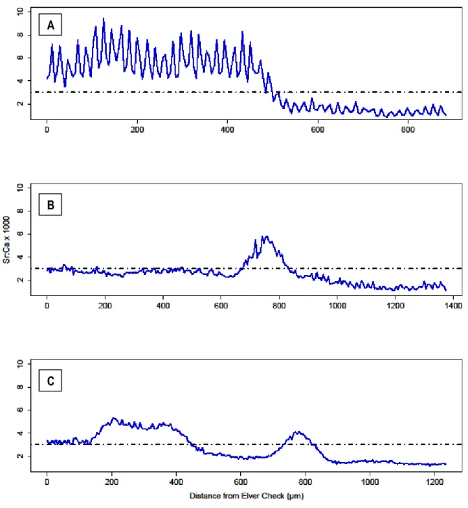
Figure 1 The Saint Lawrence River Lake Ontario system including Lake Champlain. Dashed red lines mark the limits of fluvial estuary. The river lies upstream from the upper limit while the brackish estuary begins downstream from the lower limit. Yellow dots indicate capture locations for eels collected between September 2010 and October 2011. Note that eels listed as being from Lake Ontario were in fact captured in the brackish estuary... 50 Figure 2 : Image of a stained eel otolith sectioned and polished in the transverse plane. Red dots indicate growth rings and represent one year’s worth of growth. The age estimate for this individual is 9 years. ... 51 Figure 3 : Cluster Analysis performed on concentrations of 4 elements within each section: A) Dendrogram illustrating the three clusters B) PC scores for each section plotted in multivariate space ( group 1; group 2; group 3). Ba, Mn and Mg are all strongly negatively correlated with PC1 while Sr shows a strong positive correlation with PC2. PC1 and PC2 combine to explain ~69% of the variation. ... 53 Figure 4 : Cluster Analysis performed on concentrations of four elements within each section. PC score for each section plotted in multivariate space ( group a; group b; group c; group d; group e; group f). Ba, Mn and Mg are all strongly negatively correlated with PC1 while Sr shows a strong positive correlation with PC2. PC1 and PC2 combine to explain 69% of the variation. ... 54 Figure 5 : Proportion of individuals from each sampling location having made use of each of the six habitats defined in the second cluster analysis ... 55 Figure 6 : Water sampling locations throughout the Saint Lawrence River, Estuary and upper Gulf. The most upstream station (#43) is Stony Island at the mouth of Lake Ontario. The most downstream location is Sainte-Anne-des-Monts (#1) in the Gulf. One sample collected per location. *Map by Andrew Dolittle (DFO) ... 56 Figure 7 : Longitudinal profile of water chemistry and salinity for the Saint Lawrence River, Estuary and Gulf. Concentrations (µg. g-1) of Sr, Ba, Mnand Mg. Dashed black lines highlight the limits of each section as determined with the split moving window analysis. ... 57 Figure 8 : Three Alternative migration tactics: A) prolonged residence in estuary before entering freshwater; B) recruitment to freshwater followed by a brief incursion into the estuary; C) migrant fish moving more than once between the estuary and freshwater. The dashed line at a
xii
Sr:Ca x 1000 value of 3 indicates the presumed threshold between freshwater and brackish water... ... 60 Figure 9 : Proportion of individuals having made a habitat switch at different ages (in years). A) Age of individuals at first habitat switch. This includes all individuals having made at least one switch. B) Age of individuals at second habitat switch. This includes all individuals having made at least two habitat switches. C) Age at third habitat switch. This includes all individuals that made three habitat switches ... 62 Figure 10 : Mean length-at-age predicted by the generalized additive model (GAM) plotted with respect to sampling locations ... 64
xiv
Avant-Propos
Voici maintenant deux années et demie depuis que j’ai entamé mon projet de maîtrise au sein du laboratoire de Julian Dodson au département de biologie à l’Université Laval. Je dois dire que le temps est passé très vite et que, malgré la taille réduite du laboratoire, les moments passés en tant que membre ont certainement été parmi les plus gratifiants. Depuis un jeune âge j’ai été attiré par les poissons. Je crois qu’une des raisons principales qui explique cette attraction est le fait que le milieu aquatique dans lequel ils évoluent est un milieu, a priori, si étrange, si différent et si méconnu. En effet, c’est le mystère des poissons qui continue de susciter ma curiosité. Sans doute, ma participation à un projet de grande envergure sur un des poissons les plus mystérieux, l’anguille d’Amérique, a fait en sorte que mon expérience en tant qu’étudiant à la maîtrise soit d’autant plus enrichissante et épanouissante.
D’un point de vue professionnel, mon expérience a été extrêmement formatrice et j’ai pu apprendre à utiliser plusieurs outils qui permettent de suivre et étudier les mouvements de poissons: la microchimie des otolithes, la télémétrie acoustique et les balises satellites. J’ai eu la chance de participer à un projet de télémétrie de grande envergure qui regroupait plusieurs partenaires des différents secteurs à travers le Québec. Cela m’a permis de rencontrer des chercheurs et chercheuses très accomplis dans leurs domaines et de connaître des régions du Québec et du Canada que je n’avais jamais visitées. Je suis donc infiniment reconnaissant à mon directeur de recherche, Julian Dodson et mon co-directeur, Martin Castonguay. C’est grâce à leur confiance en moi comme candidat pour mener à terme ce projet de maîtrise que j’y ai pu participer et bénéficier de toutes les opportunités qui en ont découlé. Je les remercie pour le support, les conseils, la patience et la gentillesse qu’ils m’ont offerts tout au long de mon projet. C’est à eux que je dois ma participation à ce fascinant projet sur l’anguille. Tout au long de ce projet, j’ai aussi eu la chance de travailler de façon étroite et de développer une amitié avec Mélanie Béguer, post-doctorante sur le projet OTN. Elle n’a cessé de m’impressionner tout au long de ma participation à ce projet et je suis infiniment reconnaissant pour ses conseils, son aide et sa patience. Je tiens aussi à remercier Pascal Sirois pour m’avoir accueilli dans son laboratoire et avoir partagé son expertise sur les analyses microchimiques des otolithes.
xv
Ce projet a impliqué d’importantes collaborations avec plusieurs personnes du Ministère des ressources naturelles du Québec sans lesquelles il n’aurait pas pu se réaliser. Je tiens à remercier Denise Deschamps et Yanick Soulard pour leur aide durant les préparations de mes échantillons d’otolithes. De plus, je tiens à remercier Guy Verreault de m’avoir donné accès à des otolithes d’anguilles dont l’historique migratoire était connu. Je remercie également l’équipe de Guy Verreault, en particulier Rémi Tardif, qui m’a fourni beaucoup d’aide quant aux techniques d’estimation d’âge à partir d’otolithes d’anguilles ainsi que les grosses anguilles en provenance du Lac Ontario.
Ce projet a été financé en majeure partie par la Subvention de réseau stratégique Ocean Tracking
Network (OTN) dont le siège est à l’Université Dalhousie à Halifax. Ce réseau regroupe des
chercheurs, des étudiants gradués et des stagiaires postdoctoraux à travers le Canada qui étudient les mouvements d’organismes marins. Le financement qu’ils ont fourni dans le cadre de ce projet provient du Conseil de recherche en sciences naturelles et de génie du Canada (CRSNG). De plus, je tiens à remercier Québec Océan pour leur support financier et leur prêt d’équipement. José Benchetrit, Mélanie Béguer-Pon, Martin Castonguay, Pascal Sirois, John Fitzsimons et Julian J. Dodson sont les auteurs de l’article qui sera soumis pour publication suite à ce mémoire. J.B. est le chercheur principal et l’auteur principal de ce projet. Il a réalisé la majeure partie des analyses, toutes les figures et tableaux. M.B. est chercheure postdoctorale à l’Université Laval. Elle est co-auteure et a réalisé une partie des analyses. M.C., coauteur de ce projet et co-directeur de maîtrise, est chercheur à l’Institut Maurice Lamontagne du Ministère des Pêches et des Océans et professeur associé à l’Université Laval et l’Université du Québec à Rimouski. P.S. est coauteur et professeur titulaire en sciences fondamentales à l’Université du Québec à Chicoutimi. Il a fourni l’accès au spectromètre de masse couplé au laser à plasma induit (LA-ICP-MS) ainsi que les ressources financières pour son utilisation. J.F. est chercheur émérite au Laboratoire des sciences halieutiques et aquatiques des Grands Lacs du Ministère des Pêches et des Océans. Il est coauteur et a fourni les concentrations d’éléments dans l’eau d’eau du Saint-Laurent qui ont été prélevées par son équipe. Finalement, J.J.D. est professeur titulaire au Département de biologie de l’Université Laval. Il est le directeur de maîtrise et coauteur.
1
1. INTRODUCTION GÉNÉRALE
1.1. Concepts généraux des migrations chez les poissons
Une migration, au sens strict du terme, est un comportement de déplacement qui se manifeste à un moment déterminé durant le cycle vital d’une espèce et qui caractérise l’ensemble ou la majorité des individus de cette espèce (voir Dodson 1997). Généralement, ceci implique un déplacement entre des habitats plus ou moins bien définis et suffisamment éloignés les uns des autres (Landsborough Thompson 1942). Contrairement à des mouvements reliés à l’alimentation, de nature aléatoire et généralement initiés par des mécanismes environnementaux, les migrations sont des mouvements initiés par des mécanismes internes qui se manifestent à des moments précis durant le cycle vital d’un individu (McCleave & Edeline 2009). Selon Dingle (1980), une migration implique forcément des changements spécialisés (morphologiques, physiologiques etc.) qui sont le résultat d’une sélection naturelle agissant sur une espèce. Chez les poissons, on identifie traditionnellement trois grandes catégories de comportements migratoires qui sont catégorisés selon le milieu – marin ou eau douce – dans lequel ils ont lieu. Tout d’abord, les poissons océanodromes sont ceux qui effectuent des migrations ayant lieu exclusivement en milieu marin. Les migrations potamodromes s’effectuent, quant à elles, exclusivement en eau douce (rivières, lacs etc.). Finalement, les espèces diadromes sont celles qui effectuent des migrations entre les milieux dulcicoles et les milieux marins ou estuariens (Myers 1949). Les migrations diadromes sont particulièrement intéressantes puisqu’elles nécessitent des adaptations physiologiques spécialisées (p. ex. les adaptations osmo-régulatoires) en raison des différences prononcées de salinité entre ces milieux. Parmi les comportements migratoires diadromes, on distingue trois types différents, définis en fonction du stade du cycle vital de l’espèce durant lequel les différents habitats sont exploités. Tout d’abord, les poissons anadromes, comme plusieurs salmonidés, regroupent les espèces pour lesquelles la reproduction a lieu en milieu dulcicole mais dont la majeure partie de la croissance est complétée en milieu marin (McDowall 1997). Les poissons catadromes, comme les anguillidés, se reproduisent en milieu marin et effectuent leur croissance en milieu dulcicole. Finalement, les poissons amphidromes sont des poissons qui effectuent des migrations entre eau douce et marine pour des raisons autres que la
2
reproduction (McDowall 1987). Selon Gross et al. (1988), une différence au niveau de la productivité entre eau douce et côtiers marins, qui varie en fonction de la latitude, serait à la base de l’évolution des différents comportements diadromes. Dans les zones tropicales, on observe une productivité plus élevée en rivière qu’en milieu côtier tandis que dans les zones tempérées, on observe le patron inverse.
1.2. La catadromie et les anguillidés
La famille des anguillidés (Anguillidae) de l’ordre des anguilliformes regroupe 18 espèces de poissons serpentiformes distribuées à travers le globe. Communément connue comme les anguilles d’eau douce, les anguillidés sont les uniques membres de l’ordre à exploiter les milieux dulcicoles (Inoue et al 2010). La majorité des espèces est distribuée à travers les eaux tropicales de l’Indopacifique. De plus, des études phylogénétiques suggèrent qu’Anguilla
borneensis, de l’île de Bornéo, est la plus ancestrale des espèces existantes (Aoyama 2001). Ces
informations appuient l’hypothèse que l’ancêtre de cette famille était un poisson marin des eaux tropicales de l’archipel Indo-malais. Chacune des espèces d’anguillidés est caractérisée par un cycle de vie catadrome. Tsukamoto et al. (2002) suggère que l’ancêtre de la famille aurait commencé à exploiter les milieux estuariens de façon sporadique avant d’exploiter les milieux dulcicoles par la suite. De nos jours, la totalité des espèces de la famille conserve une aire de reproduction marine. Il existe un nombre important de poisson pour lesquels la reproduction a lieu dans les eaux du large afin d’éviter le risque élevé de prédation sur les larves et les jeunes dans les eaux côtières (Dodson 1997). Ceci, et le fait que le comportement reproducteur soit souvent conservateur, a fait en sorte que les anguillidés aient maintenues leur site de fraye dans ce milieu malgré l’éloignement progressif de leurs habitats de croissance (Tsukamoto et al. 2002). Selon ce modèle, les changements dans la configuration des plaques tectoniques expliqueraient la spéciation chez la famille ainsi que la distribution actuelle des différentes espèces qui la constituent (Tsukamoto et al. 2002). Il est intéressant de remarquer l’absence totale d’anguilles d’eau douce dans le Pacifique de l’Est et dans l’Atlantique Sud. De plus, seulement deux espèces se trouvent dans le bassin de l’Atlantique Nord, soit l’anguille d’Amérique (Anguilla rostrata) et l’anguille européenne (Anguilla anguilla).
3
1.2. Biologie générale de l’anguille d’Amérique
L’anguille d’Amérique, Anguilla rostrata (LeSueur 1873), est un poisson typiquement catadrome caractérisé par un cycle vital complexe qui implique une reproduction en milieu océanique, une phase de croissance prolongée en eaux continentales et, ultimement, une migration de retour vers le site de reproduction. Avec l’anguille européenne, Anguilla anguilla, l’anguille d’Amérique est l’un des deux seuls membres de la famille à se retrouver dans le bassin Atlantique. Tandis que la distribution de l’anguille européenne s’étend à travers les eaux continentales de la façade orientale de l’Atlantique nord, l’anguille d’Amérique, quant à elle, y est distribuée sur la façade ouest. L’aire de distribution de l’espèce est parmi les plus importantes des poissons d’Amérique et s’étend sur presque 50° de latitude, soit depuis le sud du Groenland jusqu’aux Antilles et au nord de l’Amérique du sud. À travers de cette vaste étendue géographique, on la retrouve dans divers habitats aquatiques, tant en eau douce qu’en eau saumâtre et marine (Helfman et al. 1987).
Bien qu’aucune anguille adulte n’ait jamais été observée ni échantillonnée en milieu océanique, d’importantes campagnes de recherche ont réussi à identifier le site de reproduction qui se trouve dans la partie occidentale de la Mer des Sargasses entre environ 500 et 1000km au sud-ouest des Bermudes (Schmidt 1923; McCleave et al. 1987; Kleckner & McCleave 1988). Cet endroit serait, entre autres, associé à des fronts thermiques ce qui servirait probablement de repère pour les anguilles adultes prêtes à frayer (Kleckner et al. 1983). La reproduction est synchronisée pour toutes les anguilles matures en provenance de l’ensemble de l’aire de distribution. En effet, l’espèce est constituée d’une seule population reproductrice panmictique et aucune structure spatiale génétique n’a été observée (Côté et al. 2013). Le pic de reproduction a lieu au mois de mars mais des jeunes larves sont présentes de février à avril. Pendant la phase larvaire, dite leptocéphale, qui débute à l’éclosion des œufs, la morphologie de l’individu ressemble peu à celle de l’anguille adulte. Les leptocéphales ont un corps comprimé latéralement et adapté à la vie planctonique durant laquelle elles dérivent passivement avec les principaux courants océaniques de surface vers les eaux côtières à travers leur aire de distribution. À l’approche du talus continental et des eaux côtières, en moyenne 8 mois après l’éclosion sur le
4
site de reproduction, les leptocéphales se métamorphosent et passent au stade de civelle transparente (Wang & Tzeng 2000). Malgré le fait qu’elles soient translucides, les civelles prennent désormais une forme serpentine caractéristique des anguilles adultes et entament une migration vers les côtes à travers l’aire de distribution. À l’arrivée dans les eaux côtières et les embouchures d’estuaires, certaines d’entre elles choisissent d’y rester tandis que d’autres poursuivent leur migration ver l’amont sur plusieurs années (Haro and Krueger 1999). A partir de ce moment, les civelles acquièrent progressivement une pigmentation et lorsqu’elles seront entièrement pigmentées, on les nommera anguillettes. On observe une relation positive entre la taille moyenne des anguillettes et la distance par rapport au site de fraie (Jessop 2010). À mesure qu’elles migrent, le ventre des anguilles prend éventuellement une couleur jaune ou olive et les dos est devient foncé. À ce stade on la surnomme «anguille jaune» et c’est durant ce stade que la majeure partie de la croissance aura lieu. Les anguilles jaunes utilisent une grande variété d’habitats et l’on observe une certaine variabilité quant à l’espace vital qu’elles occupent (La Bar and Facey 1983). Certaines effectuent même de mouvements saisonniers entre des zones éloignées (Medcof 1969; Jessop 1987).
1.3. Une catadromie facultative
Au cours des 15 dernières années, des recherches menées sur plusieurs espèces d’anguillidés ont démontré qu’une phase de croissance en milieu dulcicole n’est pas obligatoire et que la catadromie serait un parmi plusieurs comportements migratoires (Daverat et al. 2006; Arai & Chino 2012). En effet, certains individus ne pénètrent jamais en milieu d’eau douce et effectuent l’intégralité de leur croissance en milieux estuarien et ou marin côtier ou encore font des mouvements entre les milieux saumâtres et des milieux d’eau douce à une ou plusieurs reprises durant leur séjour continental. Les premières études qui ont visées à étudier ce phénomène se sont concentrées sur les espèces de zones tempérées : l’anguille européenne (Anguilla anguilla) (Tzeng et al. 2000; Limburg et al. 2003; Daverat & Tomas 2006), l’anguille japonaise (Anguilla japonica) (Kotake et al. 2004; Arai et al. 2009), l’anguille de Nouvelle-Zélande (Anguilla dieffenbachii) et l’anguille d’Australie (Anguilla australis) (Arai et al. 2004) ainsi que l’anguille d’Amérique (Anguilla rostrata) (Jessop et al. 2002; Morrison & Secor 2004; Lamson et al. 2006; Thibault et al. 2007). Daverat et al. (2006) et Edeline (2007) ont proposé
5
l’hypothèse que certains individus chez ces espèces exploitent les habitats estuariens et côtiers en raison d’une plus grande productivité observée par rapport aux rivières et aux milieux d’eau douce adjacents. En effet, Gross (1987) a suggéré que ces différences qui varient avec la latitude (les milieux d’eau douce étant plus productifs sous les faibles latitudes) pouvaient influencer les comportements et les tactiques migratoires de poissons diadromes. Cependant, les dernières années ont vu plusieurs travaux démontrer le même comportement chez des espèces d’anguilles tropicales (Arai & Chino 2012). Cela suggère que l’existence de différentes tactiques migratoires est un phénomène généralisé chez les espèces de la famille.
1.5. Le système hydrographique du Saint-Laurent
Le bassin hydrographique du Saint-Laurent fluvial et des Grands Lacs est vaste et composé de plusieurs tributaires qui drainent des milieux très différents dans leurs compositions lithiques (Couillard 1982; Yang et al. 1996). La section fluviale du Saint Laurent s’étend de sa source au Lac Ontario, non loin de la ville de Kingston en Ontario, jusqu’à l’Île d’Orléans en aval de la ville de Québec. Entre ces deux limites, le fleuve draine des sous-bassins versants qui varient dans leurs compositions lithiques. Les tributaires qui se déversent le long de la rive nord du fleuve (les deux principaux étant la Rivière des Outaouais et la Rivière Saint-Maurice) drainent les régions de roches ignées et métamorphiques typiques du Bouclier Canadien (Yang et
al. 1996; Rondeau et al. 2005). Les tributaires qui se déversent sur la rive sud (ex. la Rivière
Richelieu), quant-à eux, drainent des régions largement composées de roches sédimentaires. Le Lac Ontario, qui contribue à la majorité des eaux du fleuve, est un bassin lacustre qui a tendance à retenir les sédiments et les minéraux. L’aire d’étude est ainsi caractérisée par une variabilité spatiale en ce qui a trait à la composition physico-chimique des différentes masses d’eau qui la constituent. Cette variabilité pourrait contribuer à l’existence des signatures chimiques spécifiques aux différentes sections du système hydrographique. De plus, il est important de noter que les eaux du fleuve ne sont pas bien mélangées et qu’une importante stratification longitudinale existe (Frenette et al. 2003; Rondeau et al. 2005). En effet, les masses d’eaux provenant du Lac Ontario et des principaux tributaires restent séparées sur une grande partie du cours d’eau.
6
1.6. Contexte et problématique de l’étude
L’anguille a longtemps représenté une ressource importante dans le système hydrographique du Saint-Laurent et du Lac Ontario (Verreault et al. 2004). De plus, les anguilles du Saint-Laurent et du Lac Ontario sembleraient constituer une composante importante de la population totale de l’espèce. D’abord, compte tenu de l’étendue et de la taille du système hydrographique, l’écoulement du fleuve Saint-Laurent représente à lui-seul environ 19% des écoulements de l’aire de distribution de l’espèce (Castonguay et al. 1994) En effet, le rapport sur l’état et le statut de l’espèce au Canada rédigé par le COSEWIC (2012) présente une méthode d’estimation de la contribution relative d’une région à la ponte totale de l’espèce en fonction du débit d’eau douce. Bien que cette méthode ne soit pas validée, elle estime que le bassin du Saint-Laurent affiche une contribution de 48,8% à la ponte totale de l’espèce. Étant donné que les anguilles qui proviennent du Saint-Laurent et du Lac Ontario sont presque exclusivement des femelles et que celles-ci sont nettement plus grosses que leurs congénères ailleurs (Verdon et al. 2002; Verreault et al. 2002), les anguilles du haut Saint-Laurent et du Lac Ontario formeraient une composante ou un stock particulièrement importante pour l’espèce.
Depuis les années 1980, on observe des déclins importants et généralisés chez l’anguille d’Amérique à travers son aire de distribution (Castonguay et al. 1994 ; Casselman 2003). Le déclin a été particulièrement prononcé pour les anguilles du haut Saint-Laurent et du Lac Ontario. Le nombre d’anguilles matures amorçant leur migration reproductrice, mesuré par les prises d’anguilles argentées en dévalaison, ainsi que le recrutement de jeunes anguilles en phase de croissance, mesuré par le passage d’anguilles jaunes en montaison au barrage Moses-Saunders, sont les deux en déclin (Robitaille et al. 2002; Casselman 2003). D’importantes pêcheries, installées principalement entre la rive sud du fleuve du Lac Saint-Pierre jusqu’au milieu de l’estuaire, exploitent les anguilles argentées quittant leur habitats de croissance au Lac Ontario et dans le haut Saint-Laurent pour rejoindre la Mer des Sargasses (Verreault et al. 2002). Sous des efforts constants de pêches, les prises ont diminué depuis les années 1980. Bien que la cause exacte de ce déclin soit toujours ignorée, on propose plusieurs facteurs agissant seuls ou en synergie. Castonguay et al. (1994) ont tenté d’expliquer ce déclin par une surpêche commerciale, de grandes modifications anthropiques apportées au fleuve durant les années 1950 (notamment la
7
construction des barrages de Moses-Saunders et Beauharnois-Les Cèdres ainsi que les écluses de la voie maritime), la contamination des eaux et des changements par rapport aux courants marins en raison de variations climatologiques. Cependant, l’étude n’a pu déterminer une cause précise parmi ces facteurs. Verreault et al. (2004) estime que les barrages et autres obstacles anthropiques, en empêchant le libre accès à 12 140 km2 d’habitats autrefois disponibles, sont responsables du déclin généralisé dans le Saint-Laurent. En outre, Verreault et al. (2009) ont démontré que des changements climatologiques à échelles locales influencent les régimes hydrologiques qui, à leur tour, affectent le recrutement local d’anguilles dans les cours d’eau du système et que ce phénomène pourrait contribuer au déclin. Finalement, des changements climatologiques affectant les principaux courants marins de l’Atlantique Nord figurent, eux aussi, parmi les causes proposées (Bonhommeau et al. 2008).
1.7. La microchimie des otolithes
Depuis plusieurs années maintenant, les scientifiques utilisent les otolithes – petits os de l’oreille interne des poissons – dans le but d’y extraire des informations, souvent écologiques, sur une espèce ou population de poisson (Elsdon et al. 2008). L’otolithe, constitué presque entièrement de CaCO3, accroit du matériel autour d’un noyau tout au long de la durée de vie du
poisson, formant ainsi des anneaux concentriques que l’on appelle annuli. Naturellement, un des premiers objectifs des dans le domaine de l’écologie des poissons a donc a été la détermination d’âge pour ainsi comprendre la structure de la population. Au fur et à mesure que l’otolithe accroît la carbonate de calcium, des ions d’éléments mineurs et traces sont parfois incorporés par substitution au dépend des ions de Ca2+. Dans certains cas, les concentrations de ces éléments dans l’otolithe reflètent leurs concentrations dans l’eau où le poisson a évolué (Campana 1995) C’est précisément ce phénomène qui est à la base des études de microchimie des otolithes et qui permet de faire un lien entre le poisson et le milieu dans lequel celui-ci réside. Il est important de se rappeler que l’otolithe croît de façon continu durant la vie du poisson et donc assimile, tout au long de cette même période, une empreinte chimique. Une grande partie des études microchimiques ont visé à caractériser une signature chimique à un stade spécifique du cycle vital d’un poisson : dans la cœur de l’otolithe (ce qui correspond au début de la vie) afin de distinguer parmi différents stocks ou bien à la marge de l’otolithe pour avoir une idée de
8
l’environnement utilisé durant une période plus récente (Elsdon et al. 2008). Encore plus poussé, est le besoin de générer un profil chimique depuis le cœur jusqu’à la marge pour retracer l’historique des signatures chimique à travers toute la vie du poisson Les études en microchimie des otolithes ont souvent exploité différentes techniques tels que la microsonde électronique à dispersion de longueur d’onde (WD-EM), la microsonde électronique à dispersion d’énergie (ED-EM), l’émission X induite par proton (PIXE) et la spectrométrie de masse à plasma induite couplée à l’ablation par laser (LA ICP-MS). Selon Campana et al. (1997) cette dernière méthode est mieux adaptée aux études qui visent à analyser les éléments présents en faible concentration dans l’otolithe comme les éléments traces.
1.8. Objectifs de l’étude
L’objectif général de la présente étude a été de retracer l’histoire environnementale des anguilles durant leur phase de croissance dans le haut Saint Laurent et le Lac Ontario à partir de signatures chimiques dans les otolithes. Étant donné la vaste étendue du système, nous avons échantillonné des anguilles à différents endroits à travers celui-ci dont le fleuve Saint-Laurent, le Lac Ontario et le Lac Champlain. Ainsi nous avons voulu, le plus possible, tenir compte des potentielles différences dans le comportement migratoires d’un endroit à un autre. Dans un premier temps, nous avons cherché à vérifier, à partir d’une signature strontium, si certaines anguilles du Saint-Laurent démontrent un comportement de migration alternatif qui impliquerait une utilisation d’habitats estuariens durant la phase de croissance. Ensuite, nous avons cherché à aller plus loin en tentant, à l’aide d’autres éléments, de détecter des patrons de mouvements à travers des milieux d’eau douce. Finalement, nous avons voulu décrire les patrons de changements d’habitats et déterminer si des différences au niveau de la morphologie, de la condition et/ou de la croissance varient en fonction de ces patrons d’utilisation de l’habitat. Les informations sur les mouvements de l’espèce durant la phase de croissance ainsi que les aspects écologiques reliés sont non seulement intéressantes d’un point de vue fondamental, mais elles sont aussi essentielles pour la bonne gestion de l’espèce.
9
2. Using multi-element line scans of otoliths to retrace
habitat use of American eels Anguilla rostrata in the Saint
Lawrence River
2.1. INTRODUCTION
2.1.1. General biology of the American eel
The American eel, Anguilla rostrata, is a wide-ranging facultatively catadromous fish that inhabits freshwater, brackish water and coastal marine habitats on the western margin of the North Atlantic Ocean basin (Scott and Crossman 1973). Panmictic spawning (Côté et al. 2013) occurs offshore within the subtropical gyre of the North Atlantic, in the southwestern Sargasso Sea, approximately 500 to 1000 km southwest of Bermuda (Schmidt 1923; McCleave et al. 1987; Kleckner & McCleave 1988). Like other members of the anguillid family (Tsukamoto & Aoyama 1998), oceanic currents transport leptocephalus larvae to continental shelf areas throughout the species’ range where they metamorphose into glass eels and migrate actively towards coastal waters. Upon reaching the coast, glass eels begin migrating upstream while slowly becoming pigmented. The young sexually undifferentiated pigmented eels, also termed elvers, represent the earliest stage of the eel’s life in continental waters. The traditionally held view was that this extended growth phase – the yellow eel stage – was carried out exclusively in freshwater before undertaking a return migration to their oceanic spawning site. However, a number of recent studies carried out on several species of temperate anguillid eels have demonstrated that this catadromous lifecycle is not obligatory (Tsukamoto & Arai 2001; Tzeng
et al. 2002; Limburg et al. 2003; Daverat & Tomas 2006). Indeed certain yellow eels never enter
freshwater, instead spending their entire growth stage in brackish or marine waters. Moreover, some individuals switch between freshwater and brackish or marine habitats during the yellow phase (Daverat et al 2006). This same pattern of behavior was also reported for American eels from Eastern Quebec (Thibault et al. 2007), Nova Scotia (Jessop et al. 2002) and in the Northeastern United States (Morrison et al. 2003). It appears anguillid eels exhibit a certain level
10
of plasticity with respect to their habitat use. Daverat et al. (2006) noted that eels residing in the upper reaches of rivers were less likely to use estuarine or marine habitats. Furthermore, eels using brackish or marine habitats appear to show higher rates of growth than those residing exclusively in freshwater (Daverat et al. 2006). This is consistent with the current theory suggesting that such behavioral plasticity has evolved to allow eels to exploit brackish and marine habitats that tend to be more productive than freshwater habitats at higher latitudes (Edeline 2007).
2.1.2. The Situation in the Saint Lawrence River
The Saint Lawrence River and Lake Ontario (SLRLO) is a vast drainage system characterized by the presence of multiple fluvial lakes (Lac Saint-François, Lac Saint-Louis and Lac Saint-Pierre) along its main stem as well as one of the Great Lakes – Lake Ontario (Yang et
al. 1996; Centre Saint-Laurent: CSL, 1992). Historically, this system has been a highly
productive area for American eels and, despite a precipitous decline in the abundance of both recruits and out-migrating silver eels since the 1980s, continues to support a commercial fishery in the middle estuary (Verreault et al. 2004; MacGregor et al. 2009). Castonguay et al. (1994) suggested that, given that the Saint Lawrence Lake Ontario basin accounts for 19% of the runoff across the American eel’s entire range, it represents an extremely important growth habitat for the species. The upper reaches of the system lie a considerable distance from the spawning grounds in the Sargasso Sea (> 3500 km) and eels recruiting there must travel much further than conspecifics recruiting elsewhere in the species’ range. Furthermore, virtually all (99%) eels native to the SLRLO are large females (Dutil et al. 1985; Couillard et al. 1997) that have a growth stage that lasts at least 20 years – considerably longer than individuals elsewhere (Jessop 2010). Surprisingly, the existence of alternative migratory strategies has not been investigated for American eels inhabiting the SLRLO system and limited information is available describing their migratory behavior during the yellow phase in this system.
11
2.1.3. Otolith microchemistry
The challenge for studies attempting to characterize the migratory and movement patterns of organisms – in this case those of American eels – lies in the difficulty in obtaining information covering the entire life of the individuals being studied. As mentioned earlier, for American eels of the SLRLO, this often involves time frames in excess of 20 years. At these temporal scales, acoustic telemetry studies are a less than practical choice. Further complicating the matter is the large geographical extent of the SLRLO system. Otoliths, small aragonite accretions of the inner ear of teleosts, have become established tools used by researchers to retrospectively retrace ecological information of fishes (Kalish 1989; Campana 1999; Kraus & Secor 2004). Over the past couple of decades, an increasing number of researchers have sought to extract chemical information from otoliths in an attempt to address questions of increasing complexity, such as those inherent to this study, taking advantage of the increasing capabilities of modern probes (Elsdon et al. 2008). In many instances these have involved looking at the profile of one element such as strontium to track movements of diadromous fishes (Secor et al. 1995; Daverat et al. 2006). Several techniques are available to extract chemical data from otoliths (Campana et al. 1999). Running line scans using Laser ablation inductively-coupled plasma mass spectrometry (LA ICP-MS) provides a cost-effective and time-efficient means to obtaining the concentrations of multiple minor and trace elements from the core to the edge of an otolith, thus spanning the entire life of the fish (Sanborn & Telmer 2003). In this context, the broad objective of this study was to obtain multi-element line scans of otoliths from eels collected at multiple sites in the SLRLO system in an attempt to detect variation in the chemical signatures of otoliths that might be indicative of habitat changes. More specifically, this study was interested in determining if habitat shifts between freshwater and brackish water environments could be revealed through strontium signatures in the otoliths of sampled eels and if the use of other elements allowed for the detection of within-freshwater signatures. This study was also interested in relating the potential differences in habitat utilization to morphological differences. In particular, several works have revealed the existence of broad-headed and narrow-headed forms in European eels (Ide et al. 2011). Lammens & Visser (1989) and Proman & Reynolds (2000) related these two ecotypes to differences in diet and trophic position with narrow-headed eels feeding on smaller
12
soft-bodied organisms and broad-headed individuals feeding on larger organisms such as fish and hard-bodied invertebrates.
2.2. MATERIALS AND METHODS
2.2.1. Eel sampling
A total of 110 eels were sampled at six different locations in the SLRLO system between September 2010 and October 2011 (Figure 1). Eels sampled from Lac Saint Louis and Lake Champlain, were captured at night using an electro-fishing vessel in July 2011. Eels sampled from Lac Saint-Pierre, Cap Santé and Saint-Romuald, were obtained from commercial fishermen between October 2010 and August 2011. Although the aim was to predominantly select juvenile yellow-stage eels, most of those captured at Saint Romuald were likely silver eels given that they were captured late in the season (October 2010). Furthermore six large silver eels were obtained from the Quebec Ministry of Wildlife and Natural Resources (MRNF) in October 2011. These individuals were captured in the brackish estuary during their seaward outmigration. These individuals had been previously marked with PIT (passive integrated transponder) tags upstream from the Moses-Saunders dam in the vicinity of Cornwall, Ontario and we therefore considered them to have originated from Lake Ontario. All eels were frozen, stored and allowed to thaw before recording total length (TL), fresh body mass (BM), and head width (HW). Fulton’s condition factor (K) was calculated: K = BM/TL3 (Ricker 1975) and the gonadosomatic index (GSI) was computed by determining the wet mass of both gonads and dividing it by the fresh body mass (BM). Head widths were measured using digital calipers (±0.01mm) measuring the distance from one jaw hinge to the other across the skull. Head lengths were measured using digital calipers measuring from the tip of the snout to the operculum. The head width to head length ratio was then used as a measure of the individual’s head shape.
13
2.2.2. Preparation of otoliths
Sagittal otoliths were extracted using acid-washed plastic or Teflon-coated forceps from Fine Science Tools ®. Once extracted, otoliths were rinsed in three successive baths of de-ionized water and any remaining tissue was mechanically removed using acid-washed forceps. Cleaned otoliths were then allowed to dry for 24 hours and subsequently stored in acid-washed plastic Eppendorf tubes. Each otolith was individually embedded in an epoxy resin and hardener mixture (© Freeman Manufacturing and Supply Company) and sectioned in the transverse plane just above the core using a low speed Isomet saw and a diamond wafering blade from ©Buehler. The core of the sectioned otolith was subsequently exposed using 400 grit sanding paper. This involved frequent verification under a binocular microscope to avoid sanding past the core. Finally, the surface of the otolith surface was smoothed using fine grit (30 µm) lapping film in order to better visualize the core and growth rings.
2.2.3 Multi-elemental line scans of otoliths and ageing
Prepared embedded otoliths were mounted onto a petrographic slide (15 – 20 per slide) and placed inside the ablation cell of a Resolution M-50 Excimer ArF laser from ©Resonetics. The laser pulsing was set to 15 Hz at 4 mJ/pulse, a beam size of 75 µm and a displacement speed of 15 µm·s-1. The ablated material was transported to a 7700x model ICP-MS from © Agilent using Helium as a carrier gas and then ionized using Argon plasma at approximately 5730°C The laser trajectory was set, individually for each otolith, to scan from the ventral to dorsal margins (or vice versa) passing through the core. Raw data was output as an intensity signal measured in counts·s-1 for 7Li, 11B, 24Mg, 27Al, 29Si, 44Ca, 47Ti, 55Mn, 56Fe, 57Fe, 59Co, 61Ni, 63Cu, 64Zn, 69Ga,
75As, 88Sr, 95Mo, 107Ag, 110Cd, 111Cd, 133Cs, 138Ba, 140Ce, 202Hg, 208Pb and 238U. Before each
otolith the blank gas was run for 30 seconds in order to determine background counts. Before and after scanning a series of 10 transects, we ran a 30 second laser scan across the standard material (NIST 612) in order to correct for temporal drift in the sensitivity of the mass spectrometer. Following laser analyses, each otolith was polished with an aluminum oxide powder, etched with a 5% EDTA solution and stained using a 0.01% toluidine blue solution
14
following the procedure listed in Verreault (2002) in order to enhance annuli. Digital images of stained otoliths were then captured using a binocular microscope. These images (examples shown Fig. 1) were used to age each otolith by counting the annuli after the elver check to the edge. Furthermore, each otolith was observed under a binocular microscope to check for the presence of an oxytetracycline (OTC) mark indicating whether the individual had been stocked. Between 2005 and 2009, several million glass eels from Nova Scotia were marked with a fluorescent oxytetracycline tag and stocked in both Lake Ontario and Lake Champlain in an effort to reconstitute those two population segments that had virtually collapsed (Verreault et al. 2010).
2.2.4. Data analysis
Raw data, output as intensity in counts·s-1, were converted into instantaneous concentrations expressed in µg·g-1 (parts per million) for each element using NIST 612 Standard Reference Material as a calibration standard and 43Ca as an internal standard assuming a Ca43
concentration of 40% by weight in the otolith. Since the aim of this study was to characterize the movements of individuals during the continental portion of their lifecycle, elemental transects were truncated so as to exclude the high strontium values recorded inside the elver check that correspond to the leptocephalus and glass eel stages prior to recruitment in continental waters. Strontium values inside the core are extremely elevated and drop abruptly at the onset of the elver stage regardless of whether or not it enters freshwater (Lin et al. 2009). Tzeng (1996) and Otake et al. (1994) demonstrated that this drastic drop is, at least in part, related to ontogeny rather than exposure to lower ambient strontium concentrations. All elemental profiles were therefore chosen to begin at the position along each transect after which this pronounced reduction in strontium values occurred. Along each transect, there were occasional outlier values, most often the result of dust or other particulate impurities interacting with the laser. To address this issue, we determined which readings were greater than median plus three times the inter-quartile range for a window spanning seven points on either side of the value. The reading was then replaced with the median of those 14 points. We did not retain any elements whose transect profiles often fell below the limits of detection (LOD) and/or limits of quantification (LOQ). The
15
former corresponds to three times the mean blank concentration for the element considered while the latter corresponds to three times that value. Moreover, elements whose transect profiles showed little to no trend were not retained. Consequently, we decided to retain only the profiles for elements for which the concentrations remained above the limits of detection (LOD) and limits of quantification (LOQ) and showed trends in the otolith transects.
A quantitative method was then used to determine where transitions occurred in the profiles for each selected element for each otolith transect. Hedger et al. (2008) stressed the importance of using a quantitative method to establish where changes occur along the sequence of elemental profiles in otoliths. They compared the application of three different algorithms on Sr:Ca profiles of American eels in an attempt to classify movements between fresh, brackish, and sea water. One of these, developed by Webster (1973), was chosen for the analyses in this study. The algorithm consisted of running a split moving window across each of the four elemental profiles that were selected for each otolith in order to generate a series of positions along its transect where a break in the chemical profile occurred. We used an R code written by Rossiter (2009) to run the algorithm along the elemental profiles of each otolith. The window width was individually set for each transect to correspond to two thirds of the position at which the autocorrelation function fell to zero. Running the split window across each transect in this manner enabled us to divide each of these into a series of sections (mean number of sections per otolith = 5) whose chemical signatures were statistically uncorrelated. The mean values for the selected elements within each section were then calculated. To further reduce the complexity and variation in the data, we performed a hierarchical cluster analysis using Ward’s minimum variance method (Ward 1963) on the total number of mean concentration values within each section for each retained elements for all otoliths. We used the Pseudo-f criterion (Calinski & Harabasz 1974), Cubic Clustering criterion (Sarle 1983) and the Pseudo-t2 criterion (Duda and Hart 1973) to determine the appropriate number of clusters to retain from the resulting cluster dendrogram. A Principle Component Analysis on the concentrations for each section in order to visualize how the three signatures compared to one another in multivariate space. We performed a one-way ANOVA followed by pair-wise t tests on the data for each element with the group as a fixed factor. This allowed us to determine whether the groups differed with respect to each elemental signature. Prior to each ANOVA, we performed Bartlett’s test of equal variance. When
16
the variances were not equal, the data were inverse, square root, cubic root or log-transformed depending on which transformation achieved equal variance. We then determined the numbers of times within one otolith transect that a switch between these three groups occurred and at what age this switch occurred. We also further explored the sub-clusters of the dendrogram groups considered in the above-mentioned analyses, specifying six groups instead of three. We performed the same PCA to visualize how these six groups compared to one another in multivariate space and compared the percentages of individuals per site for which the otolith had recorded each one these signatures.
In July 2009, water samples were collected at a total of 36 locations throughout the Saint Lawrence River, Upper Estuary and Gulf spanning more than 1000 km from Stony Island, Ontario, Canada near the outlet of Lake Ontario (Figure 6). Each water sample was collected at a depth of 1m in the middle portion of the river following the method outlined by Dove et al. (2012). The dissolved concentrations in ppm (µg·g-1) of multiple elements were analyzed for each sample. Since only one concentration value was available per location, we ran the split moving window algorithm along the longitudinal profile (i.e. upstream to downstream locations) for the concentrations of these elements. We were interested in determining whether or not we could detect sections that differed in their chemical signature and their relation to the chemical signatures detected in the otoliths of sampled eels.
2.3. RESULTS
2.3.1. Characterization of chemical signatures
Elemental concentrations for 7Li, 11B, 47Ti, 69Ga, 95Mo, 107Ag, 133Cs, 140Ce, 202Hg and
238U often fell below the limits of detection and/or limits of quantification. Moreover, otolith line
scan profiles for 27Al, 29Si, 56Fe, 57Fe, 59Co, 61Ni, 63Cu, 64Zn, 75As, 110Cd, 111Cd and 208Pb showed little to no trend. As a result, the profiles for the above-mentioned elements were deemed unsuitable for the interpretation of chemical signatures indicative of movement and were therefore not further considered. The profiles for 88Sr (strontium), 138Ba (barium), 55Mn (manganese) and 24Mg (magnesium) were all above the limits of detection and limits of
17
quantification and showed patterns of variation across the otolith transects. Consequently, the profiles for these four trace elements were retained for subsequent analyses.
Three groups were formed from the cluster analysis on the means of each elements within all sections established using the split moving window algorithm (Figure 3a). The principal component analysis enabled us to plot each section’s assigned group in multivariate space (Figure 3b). The first principle component showed a strong negative correlation with Ba, Mn and Mg (PC1 loadings: -0.496, -0.615, -0.613 respectively) while the second component was strongly correlated with Sr (PC2 loading; 0.985). Together, the first two principle components (PC1 and PC2) explained approximately 70% of the total variation. Significant differences were detected for Sr among the three groups (F = 270.95, df = 2, P < 0.001). The first group had a Sr signature that was ca 3 times greater than groups 2 and 3 (pair-wise t test, P < 0.001) (Table 1). Group 2 had a slightly greater Sr signal than group 3 (pair-wise t test, P = 0.0012). We calculated the mean Sr:Ca ratio for group 1 by dividing the mean Sr concentration of the group by the presumed concentration of Ca43 (40% wt = 4.0 x 10⁵ ppm). We obtained a value of 4.7 x
10-3, a measure more readily compared with values from other studies which did not directly use concentration data (ppm). Jessop et al. (2012) highlights the different threshold values separating freshwater and brackish water established in different studies. These range from 2.5 x 10⁻³ to 4.0 x 10⁻³. Thibault et al. (2007) and (Jessop et al. 2012) established a threshold of 3.5 x 10⁻³ that separates freshwater and brackish water signatures in the otolith. The mean value (4.7 x 10⁻³) for habitat 1 is well above this threshold value, indicating that habitat 1 likely corresponds to brackish water.
We detected significant differences in Barium signature among all three groups (F = 188.37, df = 2, P < 0.001) with group 1 having the lowest Barium signature, group 3 an intermediate signature and group 2 the highest Ba signature (pair-wise t tests, P < 0.001). Significant differences in Mn signatures among the three groups were also detected (F = 203.51, df = 2, P < 0.001) with group 2 having a mean Mn signature almost 2 times greater than groups 1 and 2 (pair-wise t tests, P < 0.001). The mean Mn signature for groups 1 and 3 were not found to be different. The Mg signature was significantly different between group 1 and 3 (P < 0.001). We found significant differences between the groups for Mg signatures (F = 99.34, df = 2, P <
18
0.001). Group 2 had a higher mean Mg value than groups 1 and 3 (pair-wise t tests, P < 0.001) and no differences were found between the latter two groups.
In summary, three distinct chemical signatures were quantified. Signature 1 was characterized by high Sr values and low Ba, Mn and Mg values. Signature 2 was characterized by low Sr values and high Ba, Mn and Mg values. Finally, signature 3 was characterized by low Sr values, intermediate Ba values and low Mn and Mg values. Given the high Strontium/low Barium signature of habitat 1, it would appear that this habitat likely corresponds to the brackish estuary. Conversely, the much lower values of Sr observed for signatures 2 and 3 likely indicate that these both correspond to two distinct freshwater signatures. From this point forward, these three signatures will be referred to as habitats 1, 2 and 3.
2.3.2. Chemical signatures beyond three clusters
Although each of the three criteria suggested retaining three of the groups from the cluster analysis, the cluster dendrogram (Figure 3a) also exhibited finer-scale structure below the level of these three groups that warranted closer examination. The considerable spread in the data along the first principle component axis (Figure 3b) that corresponds to the two freshwater signatures further illustrates this finer scale structure that goes unnoticed when considering only three groups. Considering six groups (a-f, Figure 4), plotted in the same multivariate space, it is possible to observe that group 2 is comprised of two sub-clusters while group 3 is comprised of three sub-clusters (Figure 4). Group a still corresponds to the original group 1 – the estuarine habitat. It has a much higher Sr signature than the other 5 groups (P <0.001). Group b and f both have a similar Sr signature that is significantly higher (P < 0.001) than those of group c, d and e. The Sr signature of group c was significantly greater (P < 0.05) than that of group d. No difference was observed between the Ba signatures of group c and d. A weak difference (P = 0.0405) was found between groups b and e. Group b, c, d, e and f all spread out along the first principal component axis (Figure 4). Groups e and f both exhibited the greatest values for Ba, Mn and Mg. Indeed these two groups represented the two sub-clusters of group 2 defined above. For all other groups, we observed significant differences in Ba signatures between one another.
19
The overall pattern showed group f with the highest Ba followed by intermediate signatures for groups b and e. The Ba signature of group c was lower yet while groups a and d exhibited the lowest signatures. With respect to Mn signatures, groups a, b and d were not found to be different whereas a and c were significantly different from each other (P < 0.05). All other groups differed significantly in their Mn signal (P < 0.001). The Mn signature was greatest for group e with groups c and f having intermediate values. Finally, groups a and b had similar Mg signatures that was lower than groups 5 and 6 also found to be have the same signature. All other groups differed among each other with respect to their Mg signature.
2.3.3. Variation in water chemistry
Running the split moving window along the longitudinal profiles of strontium, barium, manganese and magnesium we detected three breaks in the data, thereby dividing the Saint Lawrence profile into four sections (Figure 7). The most downstream section showed elevated salinity values, typical of brackish waters as well as much higher Sr values and lower Ba values. This is consistent with correlations between each of these two elements and salinity. A second section, between the city of Montreal and the upstream limit of the brackish estuary exhibited elevated Ba, elevated Mn and lower Sr. A third section was detected between the upstream limit of Lac Saint François (fluvial lake) and the Island of Montreal. This section exhibited similar Ba concentrations lower Mn values. Finally, comprising the areas sampled upstream from Lac Saint François, the fourth section was characterized by even lower concentrations of Mn, while its Ba concentration was similar to the previous two freshwater sections.
2.3.4. Patterns of use of the three principal habitats
Of the 110 eels sampled, only 11 (10%) used habitat 1, the brackish estuary, and of these, all were sampled at the three most downstream sites (5 from Bécancour, 3 from Cap Santé and 3 from Saint-Romuald) (Table 3). However, when taking into account only individuals sampled at these three downstream sites, this represents 18.6% of individuals. The vast majority (90%) of
20
eels enter freshwater in the first year after the transition from the glass eel phase to the elver phase and remain in freshwater (Table 3). Three alternative tactics were observed, differing from this typically catadromous behavior (Figure 8). Seven individuals spent an extended period of time (1 – 5 years) in the estuary before entering freshwater (habitats 2 or 3). Three individuals entered freshwater and eventually made a brief incursion into the estuary before finally returning to freshwater. One individual, captured at Cap Santé, spent an extended period in the estuary before entering freshwater. This was followed by a return to the estuary after 4 years and, finally, a return to freshwater 1 year later. None of the individuals from Lake Ontario, Lac Saint-Louis or Lake Champlain made use of habitat 1. Nearly half (44.5%) the eels in the sample used habitat 2 at some time during their growth stage whereas 100% of the eels sampled used habitat 3 (Table 3). With the exception of eels sampled at Bécancour, more than 50% of the individuals sampled at each of the other locations made use of habitat 2. Overall, 28.2% of eels sampled did not switch habitats after the elver check (Table 4). While one individual from Lake Champlain made five habitat switches, the eels sampled appeared to make a maximum of three habitat switches; 44.6% of all individuals made one switch as opposed to 17.3% that made two switches and only 9.10% that made three switches. Of the eels that made one habitat switch, 87.5% moved from habitat 2 to 3. Of those that made two switches, 55% moved from habitat 2 to 3 and back to 2 while 25% moved from habitat 3 to 2 and back to 3. Most (90.1%) of the individuals that made three habitat switches moved from habitat 2 to 3 to 2 and back to 3. The vast majority of individuals (93.4%) made their first habitat switch within the first four years after the elver check (Figure 9a). Furthermore, the majority of eels (75.8%) having made two or more switches, made their second switch within the first four years after the elver check (Figure 9b) while, the same was true for 90% of individuals that made their third switch (Figure 9c).
2.3.5. Patterns of secondary habitat use in freshwater.
When considering the sub-structure of the two principal freshwater habitats, habitat 3 was comprised of three secondary habitats (a, b & c) while cluster 2 was comprised of two secondary habitats (e & f). We observed differences among capture sites for habitat switches between the 5 secondary habitats. In other terms, the two principal habitats (2 and 3) involve different
21
movements when considering secondary habitats (b, c, d, e and f) depending on the location of capture. The proportion of otolith sections assigned to each one of these six groups was plotted with respect to sampling location (Figure 5). With the exception of habitat a which is only observed to be used by individuals from the three most downstream sites, each one of the five other habitats was used in some proportion by individuals sampled at each one of the sites. We performed Person’s chi-squared tests to assess differences, with respect to location, in the percentages of use of each of the six habitats. Since habitat a was only used by individuals from three of the six sites, we omitted it from this test. We found significant differences between each paired location comparison (P < 0.05) with the exception of the comparison of Lac Saint-Louis and Saint-Romuald. The majority of switches between habitats 2 and 3 for eels from Lake Champlain involved movements between secondary habitats e/f and secondary habitat c. For Lac Saint-Louis and Saint-Romuald eels these switches were between f and d & b. Lake Ontario eels made switches predominantly between e and b & d whereas the switches made by Cap Santé fish tended to be among all five secondary habitats. Finally, Bécancour eels that showed little use of habitat 3, mostly switched between secondary habitats b and d.
2.3.6. Differences in morphological characteristics
All of the eels sampled from Lake Champlain were confirmed to be non-natural recruits to the system through the presence of an OTC mark distinguishing them from natural recruits. Furthermore, two eels from Cap Santé and one from Saint-Romuald were also found to have an OTC mark. However, for these three individuals, it was not possible to confirm if they had been stocked in Lake Champlain or Lake Ontario. Indeed, pair-wise t tests showed that the mean total lengths (TL) for eels sampled at Bécancour, Saint-Romuald and Lake Ontario (Table 6) was significantly greater than that of eels sampled at Lake Champlain, Lac Saint-Louis and Cap Santé (P < 0.001) (Table 6). Eels captured at Bécancour were found to have a similar mean mass (W) as those from Lac Saint-Louis, Saint-Romuald and Lake Ontario. Once again, the mean mass of eels captured at Cap Santé and Lake Champlain were similar and smaller than those from Bécancour, Lac Saint-Louis, Saint-Romuald and Lake Ontario (P < 0.001). The mean mass of eels from Saint-Romuald and Lac Saint-Louis were smaller than that of eels from Lake