HAL Id: hal-01123756
https://hal.archives-ouvertes.fr/hal-01123756v2
Submitted on 26 Jun 2018
HAL is a multi-disciplinary open access
archive for the deposit and dissemination of
sci-entific research documents, whether they are
pub-lished or not. The documents may come from
teaching and research institutions in France or
L’archive ouverte pluridisciplinaire HAL, est
destinée au dépôt et à la diffusion de documents
scientifiques de niveau recherche, publiés ou non,
émanant des établissements d’enseignement et de
recherche français ou étrangers, des laboratoires
Efficient similarity-based data clustering by optimal
object to cluster reallocation
Mathias Rossignol, Mathieu Lagrange, Arshia Cont
To cite this version:
Mathias Rossignol, Mathieu Lagrange, Arshia Cont. Efficient similarity-based data clustering by
optimal object to cluster reallocation. PLoS ONE, Public Library of Science, 2018. �hal-01123756v2�
Efficient similarity-based data clustering by optimal object to
cluster reallocation
Mathias Rossignol1Y, Mathieu Lagrange2*Y, Arshia Cont1‡
1 Ircam, CNRS, Paris, France
2 Ls2n, CRNS, Ecole Centrale Nantes, Nantes, France YThese authors contributed equally to this work.
‡This author contributed to the writing of the manuscript. * [email protected]
Abstract
We present an iterative flat hard clustering algorithm designed to operate on arbitrary similarity matrices, with the only constraint that these matrices be symmetrical. Although functionally very close to kernel k-means, our proposal performs a maximization of average intra-class similarity, instead of a squared distance
minimization, in order to remain closer to the semantics of similarities. We show that this approach permits the relaxing of some conditions on usable affinity matrices like semi-positiveness, as well as opening possibilities for computational optimization required for large datasets. Systematic evaluation on a variety of data sets shows that compared with kernel k-means and the spectral clustering methods, the proposed approach gives equivalent or better performance, while running much faster. Most notably, it significantly reduces memory access, which makes it a good choice for large data collections. Material enabling the reproducibility of the results is made available online.
Introduction
1Clustering collections of objects into classes that bring together similar ones is probably 2
the most common and intuitive tool used both by human cognition and artificial data 3
analysis in an attempt to make that data organized, understandable, manageable. 4
When the studied objects lend themselves to this kind of analysis, it is a powerful way 5
to expose underlying organizations and approximate the data in such a way that the 6
relationships between its members can be statistically understood and modeled. Given a 7
description of objects, we first attempt to quantify which ones are “ similar ” from a 8
given point of view, then group those n objects into C clusters, so that the similarity 9
between objects within the same cluster is maximized. Finding the actual best possible 10
partition of objects into clusters is, however, an NP-complete problem, intractable for 11
useful datasets sizes. Many approaches have been proposed to yield an approximate 12
solution: analytic, iterative, flat or hierarchical, agglomerative or divisive, soft or hard 13
clustering algorithms, etc., each with their strengths and weaknesses [1], performing 14
better on some classes of problems than others [2, 3]. 15
Iterative divisive hard clustering algorithms, usually perform well to identify 16
high-level organization in large data collections in reasonable running time. For that 17
focus in this paper. If the data lies in a vector space, i.e. an object can be described by 19
a m-dimensional feature vector without significant loss of information, the seminal 20
k-means algorithm [4] is probably the most efficient approach, since the explicit 21
computation of the cluster centroids ensure both computational efficiency and 22
scalability. This algorithm is based on the centroid model, and minimizes the intra 23
cluster Euclidean distance. As shown by [5], any kind of Bregman divergence, such as 24
the KL-divergence [6] or the Itakura-Saito divergence [7], may also be considered to 25
develop such efficient clustering algorithms. 26
However, for many types of data, the projection of a representational problem into 27
an vector space cannot be done without significant loss of descriptive efficiency. To 28
reduce this loss, specifically tailored measures of similarity are considered. As a result, 29
the input data for clustering is no longer a n × m matrix storing the m-dimensional 30
vectors describing the objects, but a (usually symmetric) square matrix S of size n × n 31
which numerically encodes some sort of relationship between the objects. In this case, 32
one has to resort to clustering algorithms based on connectivity models, since the 33
cluster centroids cannot be explicitly computed. 34
Early attempts to solve this issue considered the k-medoids problem, where the goal 35
is to find the k objects that maximize the average similarity with the other objects of 36
their respective clusters, or medoids. The Partition Around Medoids (PAM) 37
algorithm [8] solves the k-medoids problem but with a complexity of O(k(n − k)2)i, n
38
being the number of objects and i number of iterations. Due to the high complexity and 39
the low convergence rate, this algorithm cannot be applied to decent size datasets. In 40
order to scale the approach, the Clustering LARge Applications (CLARA) algorithm [8] 41
draws a sample of objects before running the PAM algorithm. This sampling operation 42
is repeated several times and the most satisfying set of medoids is retained. In contrast, 43
CLARANS [9] preserves the whole set of objects but cuts complexity by drawing a 44
sample of neighbors in each search for the medoids. 45
Another classical approach to the issue is to run a variant of k-means that considers 46
average intra-cluster similarity as the guiding criterion for object-to-class 47
reallocation [10, Chapter 10.7]. This straightforward technique performs well in many 48
cases, but the complexity of computing anew intra-cluster similarities at each iteration 49
makes it impractical for large datasets. 50
Following work on kernel projection [11], that is, the fact that a nonlinear data 51
transformation into some high dimensional feature space increases the probability of the 52
linear separability of patterns within the transformed space, [12] introduced a kernel 53
version of the K-means algorithm, whose input is a kernel matrix K that must be a 54
Gram matrix, i.e. semi definite positive. [13] linked a weighted version of the kernel 55
K-means objective to the popular spectral clustering [14], introducing an efficient way of 56
solving the normalized cut objective [15]. 57
The kernel k-means algorithm proves to be equally useful when considering arbitrary 58
similarity problems if special care is taken to ensure definite positiveness of the input 59
matrix [16]. This follows original algorithmic considerations where vector space data is 60
projected into high dimensional spaces using a carefully chosen kernel function. 61
Despite such improvements, kernel k-means cannot be easily applied to large scale 62
datasets without special treatments because of high algorithmic and memory access 63
costs. [17] considered sampling of the input data, [18] considered block storing of the 64
input matrix, and a pre-clustering approach [19] is considered by [20] with a coarsening 65
and refining phases as respectively a pre- and post-treatment of the actual clustering 66
phase. 67
We show in this paper that by using a semantically equivalent variant of the average 68
intra-cluster similarity presented in [10, Chapter 10.7], it becomes possible to perform a 69
convergence for arbitrary similarity measures. Although both of those techniques are 71
well known, combining them is non trivial, and lead to a clustering algorithm, which we 72
call k-averages with the following properties: 73
• input data can be arbitrary symmetric similarity matrices, 74
• it has fast and guaranteed convergence, with a number of object to clusters 75
reallocations experimentally found to be roughly equal to the number of objects, 76
• it provides good scalability thanks to a reduced need for memory access, and 77
• on a collection of synthetic and natural test data, its results are equivalent to 78
those of kernel k-means, and obtained in a fraction of its computing time, 79
particularly when paged memory is required. 80
To summarize, the main contribution of the paper is to present a clustering 81
algorithm: 82
• that can handle arbitrary affinity matrices, i.e. semi-positiveness is not a 83
mandatory requirement for guaranteed convergence 84
• thanks to a carefully designed strategy to update the membership of objects to 85
cluster, the algorithm is fast and memory efficient. 86
The remaining of the paper is organized as follows: Section 1 presents the kernel 87
k-means objective function and the basic algorithm that minimizes this function, and 88
Section 2 introduces the concepts behind the k-averages algorithm, followed by a 89
detailed algorithmic description in Section 3. The complexity of the two algorithms in 90
terms of arithmetic operations and memory access is then studied in Section 5. The 91
above presented properties of the proposed k-averages algorithm are then validated on 92
synthetic controlled data in Section 6 and on 43 datasets of time series issued from 93
various sources in Section 7. 94
1
Kernel k-means
95Since its introduction by [12], kernel k-means has been an algorithm of choice for flat 96
data clustering with known number of clusters [16, 20]. It makes use of a mathematical 97
technique known as the “ kernel trick ” to extend the classical k-means clustering 98
algorithm [4] to criteria beyond simple euclidean distance proximity. Since it constitutes 99
the closest point of comparison with our own work, we dedicate this section to its 100
detailed presentation. 101
In the case of kernel k-means, the kernel trick allows us to consider that the k-means 102
algorithm is operating in an unspecified, possibly very high-dimensional Euclidean 103
space; but instead of specifying the properties of that space and the coordinates of 104
objects, the equations governing the algorithm are modified so that everything can be 105
computed knowing only the scalar products between points. The symmetrical matrix 106
containing those scalar products is known as a kernel, noted K. 107
1.1
Kernel k-means objective function
108In this section and the following, we shall adopt the following convention: N is the 109
number of objects to cluster and C the number of clusters; Nc is the number of objects 110
in cluster c, and µc is the centroid of that cluster. zcn is the membership function, 111
whose value is 1 if object on is in class c, 0 otherwise. In the folowing equations, µc and 112
Starting from the objective function minimized by the k-means algorithm, expressing 114
the sum of squared distances of points to the centroids of their respective clusters: 115
S = C X c=1 N X n=1 zcn(on− µc)>(on− µc)
And using the definition of centroids as: 116
µc= 1 Nc N X n=1 zcnon
S can be developed and rewritten in a way that does not explicitly refer to the 117
centroid positions, since those cannot be computed: 118
S = C X c=1 N X n=1 zcnYcn where Ycn= (on− µc)>(on− µc) = onon− 2o>nµc+ µ>cµc = o>non− 2o>n 1 Nc N X i=1 zcioi+ 1 Nc N X i=1 zcioi !> 1 Nc N X i=1 zcioi ! = o>non− 2 Nc N X i=1 zcio>noi+ 1 N2 c N X i=1 N X j=1 zkizkjo>i oj = Knn− 2 Nc N X i=1 zciKni+ 1 N2 c N X i=1 N X j=1 zkizkjKij (1)
Since the sum of Knn over all points remains constant, and the sum of squared 119
centroid norms (third, quadratic, term of Equation 1) is mostly bounded by the general 120
geometry of the cloud of objects, we can see that minimizing this value implies 121
maximizing the sum of the central terms, which are the average scalar products of 122
points with other points belonging to the same class. Therefore, given a matrix 123
gathering similarities between objects, if that matrix possesses the necessary properties 124
to be considered as a kernel (positive semidefinitness), then the kernel k-means 125
algorithm can be applied to it in order to create clusters that locally maximize the 126
average intra-cluster similarity. 127
1.2
Algorithm
128Finding the configuration that globally minimizes S (Eq. 1.1) is an NP-complete 129
problem. However, several approaches allow finding an acceptable approximation. We 130
shall only focus here on the fastest and most popular, an iterative assignment / update 131
procedure commonly referred to as the “ k-means algorithm ” [4], or as a discrete version 132
of Lloyd’s algorithm, detailed in Algorithm 1. 133
The version given here is the most direct algorithmic translation of the mathematical 134
foundations developed above, and as we shall see in section 5, it can easily become more 135
Data: number of objects N , number of classes C, kernel matrix K Result: label vector L defining a partition of the objects into C classes
1 Initialization: fill L with random values in [1..C]; 2 while L is modified do
3 for n ← 1 to N do 4 for c ← 1 to C do
5 Compute Ycnfollowing Eq. 1 (note: zcn= (Ln == c) ? 1 : 0)
6 end
7 Ln= argminc(Ycn); 8 end
9 end
Algorithm 1: Lloyd’s algorithm applied to minimizing the kernel k-means objective.
2
Foundations of the k-averages algorithm
137In our proposal, we adopt an alternative objective function which, unlike kernel 138
k-means, does not rely on a geometric interpretation but an explicit account of the 139
similarity matrix. The goal is to maximize the average intra-cluster similarity between 140
points, a commonly used metric to evaluate clustering quality, and one whose 141
computation is direct—linear in time. 142
Due to its simplicity, however, the objective function cannot be simply “ plugged 143
into ” the standard kernel k-means algorithm: it lacks the geometric requisites to ensure 144
convergence. We must therefore propose a specifically tailored algorithmic framework to 145
exploit it: first, we show here that it is possible to easily compute the impact on the 146
global objective function of moving a single point from one class to another; this allows 147
us to develop a greedy optimization algorithm taking advantage of that formula. 148
2.1
Conventions and objective function
149In addition to the notations presented above, we index here the set of elements 150
belonging to a given cluster ck as ck = {ok1, . . . , okNk}. For simplicity, we omit the first 151
index and note c = {o1, . . . , oNc} when considering a single class. 152
The similarity between objects shall be written s (oi, oj). We extend the notation s 153
to the similarity of an object to a class defined as the average similarity of an object 154
with all objects of the class. s(o, c) accepts two definitions, depending on whether or not 155
o is a member of c: 156 If o /∈ c, 157 s (o, c) = 1 Nc nc X i=1 s (o, oi) (2)
If o ∈ c, then necessarily ∃i | o = oi 158
s (o, c) = s (oi, c) = 1 Nc− 1 X j=1...nc,j6=i s (oi, oj) (3)
Let us call the “ quality ” of a class the average intra-class object-to-object similarity, 159
and write it Q: 160 Q (c) = 1 Nc nc X i=1 s (oi, c) (4)
In our framework, we do not explicitly refer to class centroids, preferring to directly 161
notations above, we define our objective function as the average class quality, 163
normalized with class sizes: 164
O = 1 N C X i=1 NiQ(ci) (5)
Since, informally, our goal is to bring together objects that share high similarity, a 165
first idea would be to simply repeatedly move each object to the class with whose 166
members it has the highest average similarity. This is what we call the “ naive 167
k-averages ” algorithm. 168
2.2
Naive k-averages algorithm
169Algorithm 2 presents a method that simply moves each object to the class with which it 170
has the highest average similarity, until convergence is reached. The algorithm is 171
straightforward and simple; however, experiments show that while it can often produce 172
interesting results, it also sometimes cannot reach convergence because the decision to 173
move an object to a different cluster is taken without considering the impact of the 174
move on the quality of the source cluster. 175
Data: number of objects N , number of classes C, similarity matrix S Result: label vector L defining a partition of the objects into C classes
1 Initialization: Fill L with random values in [1..C];
2 Compute initial object-class similarities S following Eq. 3 or Eq. 2; 3 while L is modified do
4 for i ← 1 to N do 5 previousClass ← Li;
6 nextClass ← argminkS(i, k) if nextClass 6= previousClass then 7 Li← nextClass;
8 for j ← 1 to N do
9 Update S(j, nextClass) and S(j, previousClass)
10 end
11 end 12 end 13 end
Algorithm 2: The naive k-averages algorithm.
To ensure convergence, we need to compute the impact on the objective function of 176
moving one object from one class to another. Using such formulation and performing 177
only reallocation that have a positive impact, the convergence of such an iterative 178
algorithm is guaranteed. 179
2.3
Impact of object reallocation on class quality
180Considering a class c, let us develop the expression of Q(c) into a more useful form. 181
Q (c) = 1 Nc Nc X i=1 1 Nc− 1 X j=1...Nc j6=i s (oi, oj) = 1 Nc(Nc− 1) Nc X i=1 X j=1...Nc j6=i s (oi, oj)
Using the assumption that the similarity matrix is symmetrical, we can reach: 183
Q (c) = 2 Nc(Nc− 1) Nc X i=2 i−1 X j=1 s (oi, oj) (6)
For future use and given the importance of the above transformation, we define: 184
Σ(c) = Nc X i=2 i−1 X j=1 s (oi, oj) Thus: 185 Q (c) = 2 Nc(Nc− 1) Σ(c) and Σ(c) =Nc(Nc− 1)Q (c) 2
2.3.1 Removing an object from a class 186
Assuming that o ∈ c, necessarily ∃i | o = oi. Since the numbering of objects is arbitrary, 187
we can first simplify the following equation by considering that o = oNc, in order to 188
reach a formula that is independent from that numbering. 189
Q (c r oNc) = 2 (Nc− 1)(Nc− 2) Nc−1 X i=2 i−1 X j=1 s (oi, oj) = 2 (Nc− 1)(Nc− 2) Σ(c) − Nc−1 X j=1 s (oNc, oj) = 2 (Nc− 1)(Nc− 2) [Σ(c) − (Nc− 1)s (oNc, c)] = 2Nc(Nc− 1)Q(c) 2(Nc− 1)(Nc− 2) −2(Nc− 1)s (oNc, c) (Nc− 1)(Nc− 2) = NcQ(c) − 2s (oNc, c) Nc− 2
The quality of a class after removal of an object is thus: 190
Q (c r o) = NcQ(c) − 2s (o, c) Nc− 2
(7) And the change in quality from its previous value: 191
Q (c r o) − Q (c) = NcQ(c) − (Nc− 2)Q(c) − 2s (o, c) Nc− 2
= 2 (Q(c) − s (o, c)) Nc− 2
2.3.2 Adding an object to a class 192
Assuming that o /∈ c, we can similarly to what has been done previously (numbering is 193
arbitrary) consider for the sake of simplicity that o becomes oNc+1 in the modified class 194
c. Following a path similar to above, we get: 195
Q(c ∪ oNc+1) = 2 Nc(Nc+ 1) Nc+1 X i=2 i−1 X j=1 s (oi, oj) = 2 Nc(Nc+ 1) [Σ(c) + Ncs (oNc+1, c)] =(Nc− 1)Q(c) + 2s (oNc+1, c) Nc+ 1
The quality of a class c after adding an object o is thus: 196
Q (c ∪ o) = (Nc− 1)Q(c) + 2s (o, c) Nc+ 1
(9) And the change in quality from its previous value: 197
Q (c ∪ o) − Q (c) = 2 (s (o, c) − Q(c)) Nc+ 1
(10)
2.4
Impact of object reallocation on the global objective
198function
199When moving an object o from class cs (“ source ”), to whom it belongs, to a distinct 200
class ct(“ target ”), (Ns− 1) objects are affected by the variation in (8), and Ntare 201
affected by that in (10); in addition, one object o moves from a class whose quality is 202
Q(cs) to one whose quality is Q (ct∪ o), as expressed by Eq. 9, which leads to an 203
impact of moving object o from class cs to class ctwich can be computed as follows: 204
δo(cs, ct) = 2Nt(s (o, ct) − Q(ct)) Nt+ 1 + 2(Ns− 1) (Q(cs) − s (o, cs)) Ns− 2 + (Nt− 1)Q(ct) + 2s (o, ct) Nt+ 1 − Q(cs) (11)
As can be seen, computing this impact is a fixed-cost operation. We can therefore 205
use the formula as the basis for an efficient iterative algorithm. 206
3
K-averages algorithm
207Our approach does not allow us to benefit, like kernel k-means, from the convergence 208
guarantee brought by the geometric foundation of k-means. In consequence, we cannot 209
apply a “ batch ” approach where at each iteration all elements are moved to their new 210
class, and all distances (or similarities) are computed at once. To guarantee 211
convergence, we must update the class properties for the two modified classes (source 212
and destination), as well as recompute the average class-object similarities for them for 213
each considered object, after finding its ideal new class. This is the principle of the 214
Data: number of objects N , number of classes C, similarity matrix S Result: label vector L defining a partition of the objects into C classes
1 Initialization: Fill L with random values in [1..C];
2 Compute initial object-class similarities S following Eq. 3 or Eq. 2; 3 Compute initial class qualities Q following Eq. 6;
4 while L is modified do 5 for i ← 1 to N do 6 previousClass ← Li;
7 nextClass ← argmaxkδi(previousClass, k) (following the definition of δ in
Eq. 11);
8 if nextClass 6= previousClass then 9 Li← nextClass;
10 Update QpreviousClassfollowing Eq. 7; 11 Update QnextClass following Eq. 9; 12 for j ← 1 to N do
13 Update S(j, nextClass) and S(j, previousClass) 14 following Eq. 12;
15 end
16 end 17 end 18 end
Algorithm 3: The K-averages algorithm.
increases complexity (and even more so for kernel k-means), in this case it leads to a 216
much improved computational performance. 217
Indeed, at a first glance, dynamically updating objectives as a result of object 218
reallocation might seem to have negative performance impact. However, our simple 219
non-quadratic updates make such dynamic changes easily tractable. New class qualities 220
are thus given by eqs. 7 and 9, and new object-class similarities can be computed by: 221
s(i, cs(t + 1)) = Ns(t).s(i, cs(t)) + s(i, n) Ns(t) + 1 s(i, ct(t + 1)) = Nt(t).s(i, cs(t)) − s(i, n) Nt(t) − 1 (12)
where i is any object index, n is the recently reallocated object, csthe “ source ” class 222
that object i was removed from, and ctthe “ target ” class that object n was added to. 223
The full description of k-averages is given in Algorithm 3. 224
4
Convergence
225The kernel k-means algorithm ensures convergence if the similarity matrix is 226
semi-definite positive. The k-averages algorithm relaxes this constraint by only 227
requiring symmetricity of the similarity matrix to ensure convergence. 228
An algorithm is guaranteed to converge if its successive iterations can be tied to a 229
strictly monotonous and bounded quantity. For the k-averages algorithm, this quantity 230
is the objective function itself, as we now show. 231
Thanks to the rewriting of the class quality function done in Eq. 6, which only 232
requires the similarity matrix to be symmetrical, we can directly define the allocation 233
implied by reallocating an object to a new class. It follows that, as long as reallocations 235
are only performed when δ > 0, O is strictly increasing throughout the execution of the 236
algorithm. 237
Moreover, O, defined as a weighted average of the average intra-class similarities for 238
the produced clusters, can be proven to never exceed the maximal similarity between 239
two objects. 240
Indeed, the average similarity of an object to other members of its class, expressed 241
as s(o, c) in Eq. 2, is an average of similarities, and therefore lower than or equal to 242
their maximum value. Similarly, the quality Q of a class, defined as the average of 243
object to class similarities (Eq. 4), is inferior to the maximum value of s(o, c), and 244
therefore to the maximum similarity between objects. Finally, O, a weighted average of 245
Q values, is, once again, inferior to their maximum value. 246
The objective function O is thus upper-bounded, and increases at each iteration of 247
the outer loop of Algorithm 3; which guarantees its convergence. 248
5
Complexity analysis
249In this section, we study the complexity of the two approaches presented above, first 250
from the point of view of raw complexity, second by focusing on memory access. 251
5.1
Computational complexity
2525.1.1 Kernel k-means 253
As can be seen in Algorithm 1, the operation on line 5 is the most costly part of the 254
algorithm: for each object n and class c, at each iteration, it is necessary to compute 255
Ycnfrom Eq. 1—an O(N2) operation in itself, per object. The impossibility of simply 256
computing the distances to a known centroid as done in the k-means algorithm leads to 257
a much higher complexity for the kernel k-means algorithm, globally O(N3) per 258
iteration, independent of how many objects are moved for that iteration. 259
It is however possible to improve the performance of kernel k-means by noting than 260
in Eq. 1, the third term of the equation, which has the highest complexity, is only 261
dependent on class definitions and not on the considered object. We can therefore 262
rewrite Eq. 1 as: 263
Ycn = Knn− 2 Nc N X i=1 zciKni+ Mc (13) where 264 Mc = 1 N2 c N X i=1 N X j=1 zkizkjKij (14)
Algorithm 1 thus becomes Algorithm 4, where the values of Mc are computed once 265
at the beginning of each loop (line 4) then reused on line 8, thus reducing the overall 266
complexity to O(n2) per iteration. This optimized version of kernel k-means is the one
267
we shall consider for performance comparison in the remainder of this article. 268
5.1.2 K-averages 269
For the k-averages method presented as Algorithm 3, the complexity of each iteration is 270
Data: number of objects N , number of classes C, kernel matrix K Result: label vector L defining a partition of the objects into C classes
1 Initialization: fill L with random values in [1..C]; 2 while L is modified do
3 for c ← 1 to C do
4 Compute Mc following Eq. 14 5 end
6 for n ← 1 to N do 7 for c ← 1 to C do
8 Compute Ycnfollowing Eq. 13 (note: zcn= (Ln== c) ? 1 : 0)
9 end
10 Ln= argminc(Ycn); 11 end
12 end
Algorithm 4: Lloyd’s algorithm applied to minimizing the kernel k-means objective, optimized version.
• O(NM) corresponding to the object-to-class similarity update at line 13, where 272
M is the number of objects moved at a given iteration. 273
In the worst case scenario, M = N , and the complexity for one iteration of the 274
algorithm remains the same as for the optimized kernel k-means algorithm, O(N2). In
275
practice, however, as can be seen on Figure 1, the number of objects moving from one 276
class to another decreases sharply after the first iteration, meaning that the complexity 277
of one iteration becomes quickly much lower than O(N2). Thus, while the first iteration 278
of k-averages has a similar complexity with kernel k-means, the overall cost of a typical 279
run of the algorithm (from 10 to 50 iterations) is much lower. 280
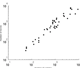
To go further in this analysis, we display on Figure 2 the total number of object 281
reallocation over a full run of the k-averages algorithm for several datatsets. The 282
datasets used to create this figure are the real-life time series data that we employ for 283
experimental validation evaluated under the Dynamic Time Warping (DTW) similarity 284
measure, cf. Section 7. As can be seen, the correlation is roughly linear with the 285
number of objects to cluster. In fact, the number of reallocations is roughly equal to the 286
number of objects to cluster, which allows us to reach for k-averages a (statistical) total 287
complexity of O(N2), instead of O(N2) per iteration.
288
5.2
Memory access
289The lowered computational costs is also accompanied by a decrease in memory access: 290
as can be seen from Equation 12, in order to compute the new object-to-class 291
similarities after moving an object n, only line n of the similarity matrix needs to be 292
read. For the remaining of the algorithm, only the (much smaller) object-to-class 293
similarity matrix is used. By contrast, in the case of kernel k-means, the computation of 294
Mc values at each iteration require that the whole similarity matrix be read, which can 295
be a serious performance bottleneck in the case of large object collections. 296
Moreover, the similarity update function of k-averages, by reading one line of the 297
matrix at a time, presents good data locality properties, which make it play well with 298
standard memory paging strategies. 299
To illustrate and confirm the theoretical complexity computed here, the next section 300
Fig 1. Number of moved objects per iteration when clustering a variety of datasets with the k-averages algorithm, normalized by the total number of objects to cluster. The datasets used to create this figure are the real-life time series data that we employ for experimental validation evaluated under the Dynamic Time Warping (DTW) similarity measure, cf. Section 7.
Fig 2. Total number of object reallocations over a run of the k-averages algorithm, plotted against the number of objects to be clustered. The datasets used to create this figure are the real-life time series data that we employ for experimental validation, cf. Section 7.
6
Validation
302In order to reliably compare the clustering quality and execution speed between the two 303
approaches, we have written plain C implementations of Algorithms 4 and 3, with 304
minimal operational overhead: reading the similarity matrix from a binary file where all 305
matrix values are stored sequentially in standard reading order, line by line, and writing 306
out the result of the clustering as a label text file. Both implementations use reasonably 307
efficient code, but without advanced optimizations or parallel processing. 308
The figures presented in this section were obtained on synthetic datasets, created in 309
order to give precise control on the features of the analyzed data: for n points split 310
between C classes, C centroids are generated at random in two dimensional space, and 311
point coordinates are generated following a Gaussian distribution around class centroids. 312
In addition to the numbers of objects and classes, the variance of Gaussian distributions 313
are adjusted to modulate how clearly separable clusters are. Similarities are computed 314
as inverse Euclidean distances between points. 315
6.1
Reproducibility
316In order to ease reproducibility of the results, the data is taken from a public repository 317
of several benchmark datasets used in academia [21] and the code of the proposed 318
method as well as the experimental code used for generated the figures is publicly 319
available1. 320
6.2
Clustering performance
321Several metrics are available to evaluate the performance of a clustering algorithm. The 322
one closest to the actual target application is the raw accuracy, that is the average 323
number of items labeled correctly after an alignment phase of the estimated labeling 324
with the reference [22]. 325
Another metric of choice is the Normalized Mutual Information (NMI) criterion. 326
Based on information theoretic principles, it measures the amount of statistical 327
information shared by the random variables representing the predicted cluster 328
distribution and the reference class distribution of the data points. If P is the random 329
variable denoting the cluster assignments of the points, and C is the random variable 330
denoting the underlying class labels on the points then the NMI measure is defined as: 331
NMI = 2I(C; K) H(C) + H(K)
where I(X; Y ) = H(X) − H(X|Y ) is the mutual information between the random 332
variables X and Y , H(X) is the Shannon entropy of X,and H(X|Y ) is the conditional 333
entropy of X given Y . Thanks to the normalization, the metric stays between 0 and 1, 1 334
indicating a perfect match, and can be used to compare clustering with different 335
numbers of clusters. Interestingly, random prediction gives an NMI close to 0, whereas 336
the accuracy of a random prediction on a balanced bi-class problem is as high as 50 %. 337
In this paper, for simplicity sake, only the NMI is considered for validations. 338
However, we found that most statements hereafter in terms of performance ranking of 339
the different algorithms still hold while considering the accuracy metric as reference. 340
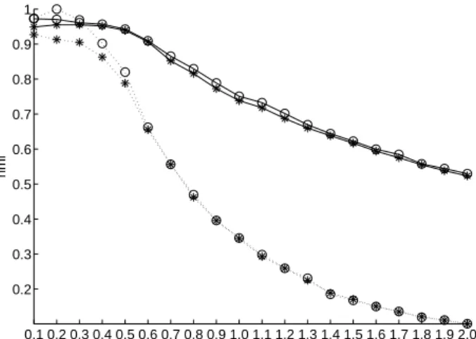
Figure 3 presents the quality of clusterings obtained using kernel k-means and 341
k-averages on two series of datasets: one featuring 5 classes, the other 40 classes. On 342
the x-axis is the variance of the Gaussian distribution used to generate the point cloud 343
0.1 0.2 0.3 0.4 0.5 0.6 0.7 0.8 0.9 1.0 1.1 1.2 1.3 1.4 1.5 1.6 1.7 1.8 1.9 2.0 0.2 0.3 0.4 0.5 0.6 0.7 0.8 0.9 1 variance nmi
Fig 3. NMI of kernel k-means (*) and k-averages (o) clustering relative to ground truth as a function of the “ spread ” of those classes for synthetic data sets of 5 and 40 classes, displayed in dashed and solid lines, respectively.
for each class: the higher that value, the more the classes are spread out and overlap 344
each other, thus making the clustering harder. 345
The question of choosing the proper number of clusters for a given dataset without a 346
priori is a well known and hard problem, and beyond the scope of this article. 347
Therefore, for the purpose of evaluation, clustering is done by requesting a number of 348
clusters equal to the actual number of classes in the dataset. In order to obtain stable 349
and reliable figures, clustering is repeated 500 times with varying initial conditions, i.e. 350
the initial assignment of points to clusters is randomly determined, and only the average 351
performance is given. For fairness of comparison, each algorithm is run with the exact 352
same initial assignments. 353
As can be seen on the figure, in the case of a 5-class problem, k-averages 354
outperforms kernel k-means in the “ easy ” cases (low class spread), before converging to 355
equivalent results. For the more complex 40-class datasets, k-averages consistently 356
yields a better result than kernel k-means, especially for higher values of the variance. 357
The lower values of NMI for 5-class experiments is in fact an artifact introduced by the 358
normalization of NMI, and is not important here; we only focus, for each series of 359
experiments, on the relative performances of kernel k-means and k-averages. 360
6.3
Time efficiency
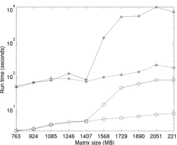
361Figure 4 shows the average time spent by kernel k-means and k-averages to cluster 362
synthetic datasets or varying sizes. As previously, initial conditions on each run are 363
identical for both algorithms. The reported run time is the one measured on a 64 bits 364
Intelr Core™ i7 runnning at 3.6 GHz with 32 Gb of RAM and standard Hard Disk 365
Drive (HDD) operated by standard Linux distribution. For results with 2 GB of RAM, 366
the same machine is used with a memory limitation specified to the kernel at boot time. 367
These figures confirm the theoretical complexity analysis presented in Section 5: 368
k-averages runs at least 20 times faster on average than kernel k-means in ordinary 369
conditions, when available memory is not an issue. When the matrix size exceeds what 370
can be stored in RAM and the system has to resort to paged memory, as in the 371
presented experiments when the matrix reaches about 1500MB, both algorithms suffer 372
from a clear performance hit; however, kernel k-means is much more affected, and the 373
Fig 4. Average computation time of the kernel k-means (*) and kaverages (o) algorithms on computers with 2 GB (solid line) and 32 GB (dashed line) of RAM, respectively. The “ running time ” axis follows a logarithmic scale.
memory-limited computer, k-averages runs about 100 times faster than kernel k-means. 375
Having established the interest of our proposed method relative to kernel k-means on 376
synthetic object collections, we now proceed to a thorough evaluation on real data. 377
7
Experiments
378In order to demonstrate the usefulness of k-averages when dealing with real data, we 379
have chosen to focus on the clustering of time series as the evaluation task. Time series, 380
even though represented as vectors and therefore suitable for any kinds of norm-based 381
clustering, are best compared with elastic measures [23, 24], partly due to their varying 382
length. The Dynamic Time Warping (DTW) measure is an elastic measure widely used 383
in many areas since its introduction for spoken word detection [25] and has never been 384
challenged for time series mining [26, 27]. 385
Effective clustering of time series using the DTW measure requires similarity based 386
algorithms such as the k-averages algorithm. With some care, kernel based algorithm 387
can also be considered provided that the resulting similarity matrix is converted into a 388
kernel, i.e. the matrix is forced to be semi definite positive, i.e. to be a Gram 389
matrix [28] in order to guarantee convergence. 390
7.1
Datasets
391To compare quality of clusterings obtained by the considered algorithms, we consider a 392
large collection of 43 time series datasets made publicly available by many laboratories 393
worldwide and compiled by Prof. Keogh. Thus, while all the experiments presented here 394
are performed on time series (chosen for being a good example of a data type requiring 395
similarity-based clustering, as opposed to a simple Euclidean approach), the great 396
variety in the sources and semantics of said series (bio-informatics, linguistics, 397
astronomy, gesture modeling, chemistry. . . ) gives this validation a wide foundation. 398
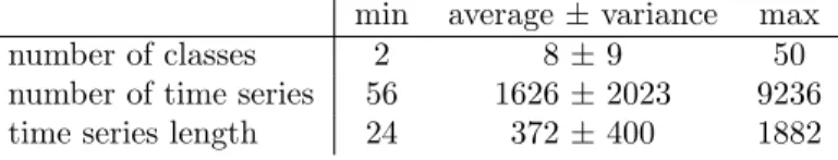
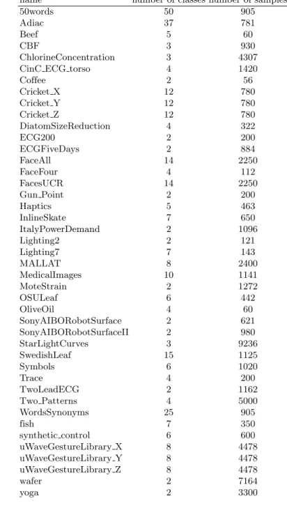
Statistics about the morphology of those datasets are summarized in Table 1. 399
Table 1. Statistics of the datasets. The length of the times series is expressed in samples.
min average ± variance max number of classes 2 8 ± 9 50 number of time series 56 1626 ± 2023 9236 time series length 24 372 ± 400 1882
7.2
Methods
401Three algorithms are considered: the spectral clustering [14] approach as a high 402
complexity reference, the kernel k-means algorithm implemented as described in Section 403
1 and the proposed k-averages algorithm. The spectral clustering algorithm tested here 404
uses the normalization proposed by Jordan and Weiss [29]. This normalization is chosen 405
over no normalization and the Shi and Malik one [15] as it is found to be the best 406
performing in terms of average NMI over all the datasets. The implementation is done 407
using the Matlab programming language. Even though a C implementation would 408
probably be more efficient, we believe that the gain would be low as the main 409
computational load is the diagonalization of the similarity matrix and the k-means 410
clustering of the eigenvectors which are both efficient builtins Matlab functions. The 411
kernel k-means is implemented both in Matlab using the implementation provided by 412
Mo Chen2 and in the C programming language following Algorithm 1. The k-averages 413
method is implemented in C following Algorithm 3. 414
7.3
Evaluation Protocol
415For each dataset, since we perform clustering, and not supervised learning, the training 416
and testing data are joined together. DTW similarities are computed using the 417
implementation provided by Prof. Ellis3 with default parameters.
418
As in our previous experiments with synthetic data, we choose here the normalized 419
mutual information (NMI) as the measure of clustering quality; clustering is done by 420
requesting a number of clusters equal to the actual number of classes in the dataset, and 421
repeated 200 times with varying initial conditions, each algorithm being run with the 422
exact same initial assignments. For the 200 clusterings thus produced, we compute the 423
NMI between them and the ground truth clustering. Average and standard deviation 424
statistics are then computed. 425
7.4
Clustering performance
426For ease of readability and comparison, the presented results are split into 3 tables. 427
Table 2 lists the results obtained on bi-class datasets, i.e. the datasets annotated in 428
terms of presence or absence of a given property; Table 3 concerns the datasets with a 429
small number of classes (from 3 to 7); and Table 4 focuses the datasets with a larger 430
number of classes (from 8 to 50). 431
For each experiment, the result of the best performing method is marked in bold. 432
The Matlab and C implementations of the kernel k-means algorithm give exactly the 433
same results in terms of NMI, thus only one column is used to display their performance. 434
A first observation is that the spectral clustering algorithm only performs favorably 435
for 2 of the 43 dataset. Also, most of the bi-class problems (Table 2) do not seem to 436
lend themselves well to this kind of approach: kernel k-means and k-averages produce 437
quasi-identical results, poor in most cases. Concerning the medium numbers of classes 438
2Available at: https://fr.mathworks.com/matlabcentral/fileexchange/26182-kernel-kmeans 3Available at: http://www.ee.columbia.edu/~dpwe/resources/matlab/dtw
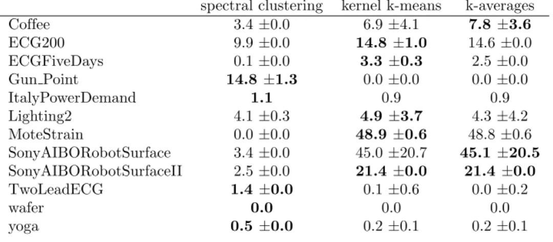
Table 2. NMI (in percents) of clusterings by kernel k-means and k-averages for bi-class datasets.
spectral clustering kernel k-means k-averages
Coffee 3.4 ±0.0 6.9 ±4.1 7.8 ±3.6 ECG200 9.9 ±0.0 14.8 ±1.0 14.6 ±0.0 ECGFiveDays 0.1 ±0.0 3.3 ±0.3 2.5 ±0.0 Gun Point 14.8 ±1.3 0.0 ±0.0 0.0 ±0.0 ItalyPowerDemand 1.1 0.9 0.9 Lighting2 4.1 ±0.3 4.9 ±3.7 4.3 ±4.2 MoteStrain 0.0 ±0.0 48.9 ±0.6 48.8 ±0.6 SonyAIBORobotSurface 3.4 ±0.0 45.0 ±20.7 45.1 ±20.5 SonyAIBORobotSurfaceII 2.5 ±0.0 21.4 ±0.0 21.4 ±0.0 TwoLeadECG 1.4 ±0.0 0.1 ±0.6 0.0 ±0.2 wafer 0.0 0.0 0.0 yoga 0.5 ±0.0 0.2 ±0.1 0.2 ±0.1
Table 3. NMI (in percents) of clusterings by kernel k-means and k-averages for datasets of 3 to 7 classes.
spectral clustering kernel k-means k-averages
Beef 25.7 ±2.4 35.5 ±2.8 34.5 ±2.6
CBF 11.1 ±0.2 41.0 ±8.4 41.0 ±7.0
ChlorineConcentration 3.9 ±0.0 0.2 ±0.1 0.2 ±0.1 CinC ECG torso 37.9 ±0.5 24.2 ±1.5 24.6 ±1.6 DiatomSizeReduction 45.3 ±4.2 79.8 ±6.3 77.3 ±4.5 FaceFour 49.8 ±4.6 72.2 ±8.4 74.9 ±6.3 Haptics 3.0 ±0.5 9.7 ±1.3 9.4 ±1.2 InlineSkate 4.6 ±0.5 6.3 ±0.7 6.4 ±0.7 Lighting7 27.6 ±2.7 51.0 ±3.1 51.3 ±1.5 OSULeaf 22.9 ±0.8 22.9 ±2.2 23.0 ±2.5 OliveOil 10.6 ±2.2 32.4 ±8.6 30.6 ±7.8 StarLightCurves 54.3 ±0.0 60.3 ±0.4 60.3 ±0.0 Symbols 72.0 ±1.7 79.1 ±3.8 79.5 ±1.6 Trace 13.7 ±4.4 54.5 ±5.1 54.3 ±6.3 Two Patterns 0.2 ±0.0 10.1 ±10.0 8.8 ±9.9 fish 18.5 ±1.5 34.9 ±1.4 35.3 ±1.0 synthetic control 63.0 ±0.7 85.3 ±4.9 89.5 ±0.8
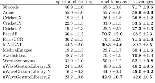
Table 4. NMI (in percents) of clusterings by kernel k-means and k-averages for datasets of 8 to 50 classes.
spectral clustering kernel k-means k-averages 50words 46.9 ±1.0 69.6 ±0.8 71.7 ±0.6 Adiac 55.0 ±1.0 55.7 ±1.0 58.9 ±0.6 Cricket X 19.2 ±1.1 26.1 ±1.8 26.8 ±1.2 Cricket Y 22.8 ±1.3 33.0 ±1.5 33.5 ±1.2 Cricket Z 19.2 ±1.3 25.5 ±2.2 27.3 ±1.3 FaceAll 36.4 ±1.2 70.7 ±2.0 68.2 ±2.3 FacesUCR 36.2 ±1.3 70.4 ±2.0 71.5 ±1.6 MALLAT 44.5 ±2.0 90.3 ±4.6 89.2 ±3.5 MedicalImages 19.2 ±1.3 29.7 ±1.7 30.4 ±1.6 SwedishLeaf 48.7 ±1.4 70.3 ±1.9 70.8 ±1.4 WordsSynonyms 31.9 ±1.0 50.9 ±1.2 52.1 ±0.8 uWaveGestureLibrary X 24.4 ±0.6 46.0 ±1.2 46.2 ±0.5 uWaveGestureLibrary Y 16.2 ±0.3 44.9 ±0.4 45.0 ±0.2 uWaveGestureLibrary Z 23.2 ±0.6 42.9 ±0.7 42.6 ±0.5
(Table 3), k-averages performs best for 8 datasets out of 17. For the larger numbers of 439
classes (Table 4), k-averages performs best for 11 datasets out of 14. 440
Considering the standard deviation over the several runs of the algorithm with 441
different initialization is helpful to study the sensitivity of the algorithm to its 442
initialization and thus its tendency to be stuck into local minima. For most datasets, 443
the standard deviation of the k-averages algorithm is smaller than the one of the kernel 444
k-means one and thus seems experimentally more robust. 445
7.5
Efficiency
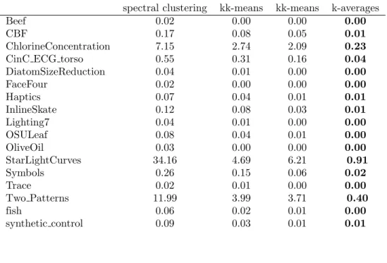
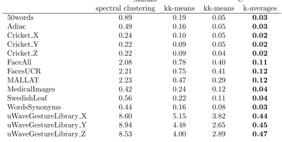
446Computation time displayed in Tables 5, 6, and 7 is the average duration over 100 runs 447
on a single core with no parallelization capabilities. For every datasets, the spectral 448
clustering approach is the more time consuming due to the diagonalization of the matrix 449
which is of O(N3). For the kernel k-means algorithm, the C implementation is most of
450
the time more efficient than the Matlab implementation. The k-average algorithm is 451
more efficient for 46 datasets out of the 47 by close to an order of magnitude for the 452
larger datasets. 453
7.6
Overall results
454To conclude on the performance of the evaluated algorithms on real datasets, Table 8 455
displays the NMI and computation time averaged over the 47 datasets. The k-averages 456
method marginally improve the clustering accuracy compared to the kernel k-means 457
approach by using less time to compute. 458
8
Conclusion
459We have presented k-averages, an iterative flat clustering algorithm that operates on 460
arbitrary similarity matrices by explicitly and directly aiming to optimize the average 461
intra-class similarity. Having established the mathematical foundation of our proposal, 462
including guaranteed convergence, we have thoroughly compared it with widely used 463
standard methods: the kernel k-means and the spectral clustering techniques. We show 464
Table 5. Computation time (in seconds) for several implementations of the evaluated clustering algorithms for datasets of 2 classes.
Matlab C
spectral clustering kk-means kk-means k-averages
Coffee 0.02 0.00 0.00 0.00 ECG200 0.03 0.00 0.00 0.00 ECGFiveDays 0.13 0.10 0.06 0.01 Gun Point 0.02 0.00 0.00 0.00 ItalyPowerDemand 0.20 0.07 0.05 0.01 Lighting2 0.02 0.00 0.00 0.00 MoteStrain 0.33 0.11 0.08 0.01 SonyAIBORobotSurface 0.09 0.02 0.01 0.00 SonyAIBORobotSurfaceII 0.09 0.01 0.02 0.01 TwoLeadECG 0.13 0.16 0.10 0.02 wafer 19.62 0.72 1.04 0.39 yoga 3.55 0.80 0.66 0.10
Table 6. Computation time (in seconds) for several implementations of the evaluated clustering algorithms for datasets of 3 to 7 classes.
Matlab C
spectral clustering kk-means kk-means k-averages
Beef 0.02 0.00 0.00 0.00
CBF 0.17 0.08 0.05 0.01
ChlorineConcentration 7.15 2.74 2.09 0.23
CinC ECG torso 0.55 0.31 0.16 0.04
DiatomSizeReduction 0.04 0.01 0.00 0.00 FaceFour 0.02 0.00 0.00 0.00 Haptics 0.07 0.04 0.01 0.01 InlineSkate 0.12 0.08 0.03 0.01 Lighting7 0.04 0.01 0.00 0.00 OSULeaf 0.08 0.04 0.01 0.00 OliveOil 0.03 0.00 0.00 0.00 StarLightCurves 34.16 4.69 6.21 0.91 Symbols 0.26 0.15 0.06 0.02 Trace 0.02 0.01 0.00 0.00 Two Patterns 11.99 3.99 3.71 0.40 fish 0.06 0.02 0.01 0.00 synthetic control 0.09 0.03 0.01 0.01
Table 7. Computation time (in seconds) for several implementations of the evaluated clustering algorithms for datasets of 8 to 50 classes.
Matlab C
spectral clustering kk-means kk-means k-averages
50words 0.89 0.19 0.05 0.03 Adiac 0.49 0.16 0.05 0.03 Cricket X 0.24 0.10 0.05 0.02 Cricket Y 0.22 0.09 0.05 0.02 Cricket Z 0.22 0.09 0.04 0.02 FaceAll 2.08 0.78 0.40 0.11 FacesUCR 2.21 0.75 0.41 0.12 MALLAT 2.23 0.47 0.29 0.12 MedicalImages 0.42 0.24 0.12 0.04 SwedishLeaf 0.56 0.22 0.11 0.04 WordsSynonyms 0.44 0.16 0.08 0.03 uWaveGestureLibrary X 8.60 5.15 3.82 0.44 uWaveGestureLibrary Y 8.94 4.48 2.65 0.45 uWaveGestureLibrary Z 8.53 4.00 2.89 0.47
Table 8. Performances averaged over the 47 datasets. The NMI is expressed in percents and the computation time in seconds.
Matlab C
spectral clustering kk-means kk-means k-averages
nmi (%) 22.1 36.6 36.6 36.8
conditions) and leads to equivalent or better clustering results for the task of clustering 466
both synthetic data and realistic times series taken from a wide variety of sources, while 467
also being more computationally efficient and more sparing in memory use. 468
Acknowledgments
469The authors would like to acknowledge support for this project from ANR project Houle 470
(grant ANR-11-JS03-005-01) and ANR project Cense (grant ANR-16-CE22-0012). 471
References
1. Jain AK. Data clustering: 50 years beyond K-means. Pattern Recognition Letters. 2010;31:651–666.
2. Steinbach M, Karypis G, Kumar V, et al. A comparison of document clustering techniques. In: KDD workshop on text mining. vol. 400. Boston; 2000. p. 525–526.
3. Thalamuthu A, Mukhopadhyay I, Zheng X, Tseng GC. Evaluation and comparison of gene clustering methods in microarray analysis. Bioinformatics. 2006;22:2405–2412.
4. MacQueen JB. Some Methods for classification and Analysis of Multivariate Observations. In: Proc. of Berkeley Symposium on Mathematical Statistics and Probability; 1967.
5. Banerjee A, Merugu S, Dhillon IS, Ghosh J. Clustering with Bregman Divergences. J Mach Learn Res. 2005;6:1705–1749.
6. Dhillon IS, Mallela S, Kumar R. A Divisive Information Theoretic Feature Clustering Algorithm for Text Classification. J Mach Learn Res.
2003;3:1265–1287.
7. Linde Y, Buzo A, Gray RM. An Algorithm for Vector Quantizer Design. IEEE Transactions on Communications. 1980;28:84–95.
8. Kaufman L, Rousseeuw PJ. Finding groups in data: an introduction to cluster analysis. New York: John Wiley and Sons; 1990.
9. Ng RT, Han J. Efficient and Effective Clustering Methods for Spatial Data Mining. In: Proceedings of the 20th International Conference on Very Large Data Bases. VLDB ’94. San Francisco, CA, USA: Morgan Kaufmann Publishers Inc.; 1994. p. 144–155.
10. Duda RO, Hart PE, Stork DG. Pattern Classification (2nd Ed). Wiley; 2001. 11. Vapnik VN. The Nature of Statistical Learning Theory. New York, NY, USA:
Springer-Verlag New York, Inc.; 1995.
12. Girolami M. Mercer Kernel-based Clustering in Feature Space. IEEE Transactions on Neural Network. 2002;13(3):780–784.
doi:10.1109/TNN.2002.1000150.
13. Dhillon IS, Guan Y, Kulis B. Weighted Graph Cuts Without Eigenvectors A Multilevel Approach. IEEE Trans Pattern Anal Mach Intell.
14. Von Luxburg U. A tutorial on spectral clustering. Statistics and computing. 2007;17(4):395–416.
15. Shi J, Malik J. Normalized cuts and image segmentation. IEEE Transactions on pattern analysis and machine intelligence. 2000;22(8):888–905.
16. Roth V, Laub J, Kawanabe M, Buhmann JM. Optimal Cluster Preserving Embedding of Nonmetric Proximity Data. IEEE Trans Pattern Anal Mach Intell. 2003;25(12):1540–1551. doi:10.1109/TPAMI.2003.1251147.
17. Chitta R, Jin R, Havens TC, Jain AK. Approximate Kernel K-means: Solution to Large Scale Kernel Clustering. In: Proceedings of the 17th ACM SIGKDD International Conference on Knowledge Discovery and Data Mining. KDD ’11. New York, NY, USA: ACM; 2011. p. 895–903.
18. Zhang R, Rudnicky AI. A large scale clustering scheme for kernel K-Means. In: Pattern Recognition, 2002. Proceedings. 16th International Conference on. vol. 4; 2002. p. 289–292 vol.4.
19. Bradley PS, Fayyad UM, Reina C. Scaling Clustering Algorithms to Large Databases. In: Knowledge Discovery and Data Mining; 1998. p. 9–15.
20. Kulis B, Basu S, Dhillon I, Mooney R. Semi-supervised graph clustering: a kernel approach. Machine Learning. 2008;74(1):1–22. doi:10.1007/s10994-008-5084-4. 21. Chen Y, Keogh E, Hu B, Begum N, Bagnall A, Mueen A, et al.. The UCR Time
Series Classification Archive; 2015.
22. Kuhn HW. The Hungarian Method for the Assignment Problem. Naval Research Logistics Quarterly. 1955;2(1–2):83–97. doi:10.1002/nav.3800020109.
23. Ding H, Trajcevski G, Scheuermann P, Wang X, Keogh E. Querying and Mining of Time Series Data: Experimental Comparison of Representations and Distance Measures. Proc VLDB Endowment. 2008;1(2):1542–1552.
doi:10.14778/1454159.1454226.
24. Wang X, Mueen A, Ding H, Trajcevski G, Scheuermann P, Keogh E.
Experimental Comparison of Representation Methods and Distance Measures for Time Series Data. Data Mining Knowledge Discovery. 2013;26(2):275–309. doi:10.1007/s10618-012-0250-5.
25. Sakoe H, Chiba S. Dynamic programming algorithm optimization for spoken word recognition. IEEE Transactions on Acoustics, Speech and Signal Processing. 1978;26(1):43–49. doi:10.1109/TASSP.1978.1163055.
26. Berndt DJ, Clifford J. Using Dynamic Time Warping to Find Patterns in Time Series. In: Fayyad UM, Uthurusamy R, editors. KDD Workshop. AAAI Press; 1994. p. 359–370.
27. Rakthanmanon T, Campana B, Mueen A, Batista G, Westover B, Zhu Q, et al. Addressing Big Data Time Series: Mining Trillions of Time Series Subsequences Under Dynamic Time Warping. ACM Trans Knowl Discov Data.
2013;7(3):10:1–10:31. doi:10.1145/2500489.
28. Lanckriet GRG, Cristianini N, Bartlett P, Ghaoui LE, Jordan MI. Learning the Kernel Matrix with Semidefinite Programming. J Mach Learn Res. 2004;5:27–72. 29. Ng AY, Jordan MI, Weiss Y. On spectral clustering: Analysis and an algorithm.
A
Description of the datasets
Table 9. Description of the time series datasets used for evaluation.
name number of classes number of samples
50words 50 905
Adiac 37 781
Beef 5 60
CBF 3 930
ChlorineConcentration 3 4307
CinC ECG torso 4 1420
Coffee 2 56 Cricket X 12 780 Cricket Y 12 780 Cricket Z 12 780 DiatomSizeReduction 4 322 ECG200 2 200 ECGFiveDays 2 884 FaceAll 14 2250 FaceFour 4 112 FacesUCR 14 2250 Gun Point 2 200 Haptics 5 463 InlineSkate 7 650 ItalyPowerDemand 2 1096 Lighting2 2 121 Lighting7 7 143 MALLAT 8 2400 MedicalImages 10 1141 MoteStrain 2 1272 OSULeaf 6 442 OliveOil 4 60 SonyAIBORobotSurface 2 621 SonyAIBORobotSurfaceII 2 980 StarLightCurves 3 9236 SwedishLeaf 15 1125 Symbols 6 1020 Trace 4 200 TwoLeadECG 2 1162 Two Patterns 4 5000 WordsSynonyms 25 905 fish 7 350 synthetic control 6 600 uWaveGestureLibrary X 8 4478 uWaveGestureLibrary Y 8 4478 uWaveGestureLibrary Z 8 4478 wafer 2 7164 yoga 2 3300