Dynamic Modeling and Identification of Joint Drive with Load-Dependent Friction Model

HAL Id: hal-00583169

https://hal.archives-ouvertes.fr/hal-00583169

Submitted on 5 Apr 2011

HAL is a multi-disciplinary open access

archive for the deposit and dissemination of

sci-entific research documents, whether they are

pub-lished or not. The documents may come from

teaching and research institutions in France or

abroad, or from public or private research centers.

L’archive ouverte pluridisciplinaire HAL, est

destinée au dépôt et à la diffusion de documents

scientifiques de niveau recherche, publiés ou non,

émanant des établissements d’enseignement et de

recherche français ou étrangers, des laboratoires

publics ou privés.

with Load-Dependent Friction Model

Pauline Hamon, Maxime Gautier, Philippe Garrec, Alexandre Janot

To cite this version:

Pauline Hamon, Maxime Gautier, Philippe Garrec, Alexandre Janot. Dynamic Modeling and

Identi-fication of Joint Drive with Load-Dependent Friction Model. International Conference on Advanced

Intelligent Mechatronics, Jul 2010, Montreal, Canada. pp. 902-907, �10.1109/AIM.2010.5695815�.

�hal-00583169�

Abstract—Friction modeling is essential for joint dynamic identification and control. Joint friction is composed of a viscous and a dry friction force. According to Coulomb law, dry friction depends linearly on the load in the transmission. However, in robotics field, a constant dry friction is frequently used to simplify modeling, identification and control. That is not accurate enough for joints with large payload or inertial and gravity variations and actuated with transmissions as speed reducer, screw-nut or worm gear. A new joint friction model taking dynamic and external forces into account is proposed in this paper. A new identification process is proposed, merging all the joint data collected while the mechanism is tracking exciting trajectories and with different payloads, to get a global LS estimation in one step. An experimental validation is carried out with a prismatic joint composed of a Star high precision ball screw drive positioning unit.

I. INTRODUCTION

HE usual identification method, based on the inverse dynamic model (IDM) and least squares (LS) method, has been successfully applied to identify inertial and friction parameters of a lot of prototypes and industrial robots [1]-[10]. The kinematic Coulomb friction at non zero velocity qɺ is widely approximated by F sign q_C ( )ɺ , where F is a C

constant parameter. The identification consists in moving the robot without any load (or external force) or with constant given payloads [9].

However, according to the Coulomb law, F is a linear _C function of the contact reaction in the mechanism. It depends on the dynamic and the external forces applied through the joint drive chain. Thus, the usual identified IDM is no more accurate for joints with varying load, particularly with transmissions as industrial speed reducer, screw-nut or worm gear because their efficiency significantly varies with the transmitted force. This dependence on load has been often observed in transmission elements [15]-[19] through direct measurement procedures. Moreover, the mechanism efficiency often depends on the sense of power transfer leading to two distinct sets of friction parameters.

This paper presents a new method to identify automatically the dry friction model where F is a linear _C function of the applied force, with an asymmetrical behavior.

An experimental validation is carried out on a ball screw drive prismatic joint.

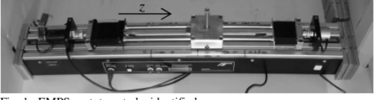
II. EXPERIMENTAL SETUP AND DYNAMIC MODEL The EMPS is a high-precision linear Electro-Mechanical Positioning System. Its main components are a Maxon DC motor which is current controlled by a four quadrant PWM amplifier, a Star high-precision low-friction ball screw drive positioning unit, and an incremental encoder. The backlash free ball screw drive is the gear converting the rotary motion of the motor to the linear carriage joint displacement. The EMPS is a standard configuration of a drive system for prismatic joint of robots, machine tools, haptic device… It is connected to a dSPACE digital control system for easy control and data acquisition using Matlab and Simulink software [20], [21].

Fig. 1. EMPS prototype to be identified.

In order to make easy variation of the gravity load, the EMPS can be fixed in vertical position alternatively with the z joint positive linear displacement in the gravity direction or in its opposite.

The inverse dynamic model is given by:

( ) ( ) ( ) a C V off out C V off I m q mg F sign q F q F sign q F q τ τ τ τ = + − + + + = + + + ɺɺ ɺ ɺ ɺ ɺ (1) where:

• q , qɺ and qɺɺ are respectively the generalized joint position, velocity and acceleration,

• τ is the drive force,

• τ_out is the output force (the load force) of the drive chain,

• Ia is the inertia moment of all rotary elements in the drive

chain (rotor of motor and encoder, ball, coupling units),

• m is the mass of all translation moving elements (screw, carriage, payload),

• FV is the viscous friction coefficient,

Dynamic Modeling and Identification of Joint Drive with

Load-Dependent Friction Model

P. Hamon

(1)

, M. Gautier

(2)

, P. Garrec

(1)

, and A. Janot

(3)

(1)

CEA, LIST, Interactive Robotics Laboratory, 18 route du Panorama, Fontenay-aux-Roses, F-92265, France. (2) _{University of Nantes/IRCCyN, 1 rue de la Noë, BP 92 101, Nantes Cedex 03, F-44321, France.} (3) _{HAPTION S.A., Atelier Relais de Soulgé, Route de Laval, Soulgé-sur-Ouette, F-53210, France.}

• FC is the Coulomb friction force,

• τ_off takes into account the amplifier offset and a dissymmetric Coulomb friction force,

• g is the projection of the gravity acceleration on the z prismatic joint axis.

• g = 9.81, when z axis stays in vertical position, oriented positive to the earth,

• g = -9.81, when z axis stays in vertical position, oriented positive to the sky.

All variables and parameters are given in SI units on the joint linear displacement side (carriage side).

III. USUAL IDENTIFICATION MODEL AND IDENTIFICATION METHOD

A. Modeling

The choice of the modified Denavit and Hartenberg frame attached to the link allows to obtain a dynamic model linear in relation to a set of standard dynamic parameters χ [6], [11]. Most of the methods to identify the joint dynamic parameters use an identification model linear in relation to the parameters, and solve the system using least squares techniques (LS) [1]-[13]. With the usual friction model, FC is

a constant (Fig. 2.a) and the inverse dynamic model (1) is linear in relation to the dynamic parameters:

[

( )

]

( ) a C V off I m m F q g sign q q 1 q,q F τ τ +         = − _{ }=       D χ ɺɺ ɺ ɺ ɺ (2)

where D(q,qɺ)=

[

qɺɺ −g sign q( )ɺ qɺ 1

]

is the regressor of the linear relation, and χ=_I_a+m m F_C F_V τ_off_T is the ( x )b 1 vector of the b base dynamic parameters.

B. Identification

We consider off-line identification of the dynamic parameters χ, given measured or estimated off-line data for τ,

q, q, qɺ ɺɺ , collected while the mechanism is tracking some planned trajectories: the inverse dynamic model (2) is sampled to get an over-determined linear system such that (3). The velocities and accelerations are calculated using well tuned band pass filtering of the joint position [6].

( )τ = (q,q,q) +

Y W ɺ ɺɺχ ρ (3)

with Y( )τ the measurements vector, W the observation

matrix and ρ the vector of errors.

The LS solution ˆχ minimizes the 2-norm of the vector of errors ρ . W is a ( x )r b full rank and well conditioned matrix where r=N_ex n, with N the number of samples on _e the trajectories. The LS solution ˆχ is given by:

(

)

-1

T T

ˆ = = +

χ W W W Y W Y (4)

It is calculated using the QR factorization of W . Standard deviations

i

ˆ χ

σ are estimated using classical and simple results from statistics. The matrix W is supposed to be deterministic, and ρ, a zero-mean additive independent noise, with a standard deviation such as:

E( T) 2 ρ σ = = ρρ r C ρρ I (5)

where E is the expectation operator and I_r, the ( x )r r

identity matrix. An unbiased estimation of σ_ρ is:

( )

2

2 _ˆ

ˆ_ρ r b

σ = Y−Wχ − (6)

The covariance matrix of the standard deviation is calculated as follows: T T -1 E ( )( ) 2( ) ˆ ˆ =  −ˆ −ˆ =σˆρ χχ C χ χ χ χ W W (7) i 2 ˆ ˆ ˆ ii χ σ =Cχχ is the i th _{diagonal coefficient of} ˆ ˆ χχ C . The

relative standard deviation

ri ˆ %σ_χ is given by: ri i ˆ ˆ ˆi %σ_χ =100σ χ_χ (8)

However, experimental data are corrupted by noise and error modeling and W is not deterministic. This problem

can be solved by filtering the measurement vector Y and the columns of the observation matrix W as in [7], [8].

IV. NEW FRICTION MODELING AND IDENTIFICATION In this section, we introduce a friction model dependent on the load and the sign of the power.

A. Load-Dependent Friction Model

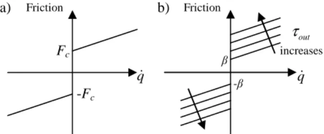
The Coulomb friction is still written F sign q_C ( )ɺ but F C

depends linearly on the absolute value of the load (Fig. 2.b), [15]-[19].

Then the inverse dynamic model becomes:

(

)

( )

out out sign q F qV off

τ τ= + α τ +β ɺ + ɺ+τ (9)

where the parameters α and β are constants to be identified. These new parameters depend on the mechanical structure of the reducers used to actuate the joint.

The inverse dynamic model can be written as follows:

( ) ( )

out out sign q sign q F qV off

τ τ= +α τ ɺ +β ɺ + ɺ+τ (10) And with τ_out =τ_outsign(τ_out), one obtains:

( ) ( ) ( )

out outsign out sign q sign q F qV off

τ τ= +ατ τ ɺ +β ɺ + ɺ+τ (11) Thus, the IDM depends on the signs of τ_out and qɺ . With

( _out) ( ) ( _out )

signτ sign qɺ =signτ qɺ , one defines 4 quadrants which can be grouped two by two (Fig. 3.a), depending on the sign of the output power denoted P_out =τ_outqɺ . In the quadrants 1 and 3, P is positive and the actuator has a _out motor behavior. In the quadrants 2 and 4, P is negative _out and the actuator has a generator behavior which may save the power to the power supply, assuming a 4 quadrants amplifier.

This model is valid for symmetrical friction. Generally, the friction is asymmetrical and α and β can take different values depending on the quadrant where the joint runs.

Fig. 2. a) Usual friction model with constant FC.

b) Parametric effect of the load on friction model. B. Power Sign-Dependent Friction Model We present here 3 ways of modeling.

• 4 models (4x1Q) for 4 different quadrants

In the general case, the friction parameters α , β, and

off

τ depend on the signs of τ_out and qɺ in the frame ( qɺ ,τout),

Fig. 3.a. That means that there are four different values for α , β and τ_off (one for each quadrant): α₁, β₁, α₂, β₂,

3

α , β₃, and α₄, β₄ (the offsets τ_off regroup with the parameters β), which defines four different models named (4x1Q). & ( ) & ( ) & ( ) & ( ) out 1 out V 1 out 2 out V 2 out 3 out V 3 out 4 out V 4 0 q 0 1 F q 0 q 0 1 F q 0 q 0 1 F q 0 q 0 1 F q τ τ α τ β τ τ α τ β τ τ α τ β τ τ α τ β > > ⇒ _{= + + +}   > < ⇒ _{= − + −}   < < ⇒ _{= + + −}   _{< > ⇒ = − + +}  ɺ ɺ ɺ ɺ ɺ ɺ ɺ ɺ (12)

• 2 models (2x2Q) for quadrants identical two by two In some cases, the friction is symmetrical with respect to the velocity and the 4 models can be simplified to 2 models. The parameters α , β and τ_off have only two different values, α_m, β_m, τ_{off m} for the motor quadrants 1 and 3 and

g

α , β_g, τ_{off g}for the generator quadrants 2 and 4.

( ) ( )

( ) ( )

out m out V m off m out g out V g off g

P 0 1 F q sign q P 0 1 F q sign q τ α τ β τ τ α τ β τ > ⇒ _{= + + + +}   < ⇒ _{= − + + +}  ɺ ɺ ɺ ɺ (13)

• 1 model (1x4Q) for 4 identical quadrants

In the case of symmetrical friction with respect to τ_out and qɺ , the models simplify to 1 model for 4 quadrants.

( ) ( )

out F qV outsign Pout sign q off

τ τ= + ɺ+ατ +β ɺ +τ (14)

Each modeling takes the load-dependency of friction into account. Starting from the (4x1Q) models, a simplification procedure based on the identification results leads to the simplest model.

However, when the joint torque amplitude is low, the friction model should be more complex because of Coulomb friction resulting from internal preload and hysteresis. Then, one cannot use the quadrants. To simplify and connect the quadrants models, a relevant approximation consists in extending them in this area which can be considered as uncertain for the experimental identification. This simplification is illustrated in a (τ ,τ_out) graph (Fig. 3.b). It should be noticed that within this area, the mechanism is no longer transmitting power which is totally dissipated in friction losses.

Fig. 3. a) Four quadrants frame (qɺ,τ_out) for motor or generator behavior. b) Asymmetrical friction for a given velocity qɺ₀ and definition of the uncertain area.

C. Friction identification method

The friction models depend on the sign of τ_out which is unknown. To overcome this problem, the samples of τ measurements are selected outside of the uncertain area (Fig. 3.b) in order to get the same sign for τ_out and τ. This allows to get the sign of P_out with:

( out) ( out ) ( ) ( )

sign P =signτ qɺ =signτqɺ =sign P (15)

The (1x4Q) modeling can be written:

( ) ( )

out F qV outsign P sign q off

τ τ= + ɺ+ατ +β ɺ +τ (16)

For the (2x2Q) modeling, 2 variables are introduced, P+ and P− defined by:

( ) 1 sign P P 2 + ₌ + _, 0 1 P> ⇔P+= , P< ⇔0 P+=0 (17) ( ) 1 sign P P P 2 − ₌ − ₌ + ₍₁₈₎ b) qɺ β -β out τ increases Friction a) qɺ Fc -Fc Friction a) qɺ Pout > 0 Motor Pout > 0 Motor Pout < 0 Generator out

τ

Pout < 0 Generator 1 4 3 2 b)

τ

_out

τ

1 Simplified and uncertain area Friction Friction 1 + αm 1 1 – αg 1 motor ge ne rato r motor ge ne rato r 0 qɺ0< 0 q0< ɺ 0 q0> ɺ 0 q0> ɺ

Then (13) can be written in one model: ( ) ( ) ( ( ) ) ( ( ) ) m out g out m off m g off g V P 1 P 1 ... ... P sign q P sign q F q τ α τ α τ β τ β τ + − + − = + + − + + + + + ɺ ɺ ɺ (19)

For the (4x1Q) modeling, 4 similar variables have to be defined to obtain one model only.

As τ_out is linear in relation to parameters, so is τ . Thus, for each friction model, one can write the IDM linear in relation to parameters and use the LS technique.

V. EXPERIMENTAL IDENTIFICATION

The identification process has been performed for the four different cases: first with the usual model where F is _C constant, then with the 3 friction models depending on the load. We have observed that the modeling with four identical quadrants (1x4Q) was insufficient because the friction is asymmetrical here. Moreover, the modeling with four different quadrants (4x1Q) was not indispensable as the parameters are very close for the two motor quadrants on one hand and for the two generator quadrants on the other hand. That is the reason why only the modeling with quadrants identical two by two (2x2Q) is detailed here and compared with the usual model. The methods for the others are very similar.

A. Data Acquisition

The identification of dynamic parameters is carried out with and without payloads: five different additional masses can be fixed on the carriage. To excite properly the friction parameters to be identified, trapezoidal velocities trajectories were used. The sample acquisition frequency for joint position and current reference (drive force) is 5 KHz.

The estimation of qɺ and qɺɺ are carried out with pass band filtering of q consisting of a low pass Butterworth filter and a central derivative algorithm. The Matlab function filtfilt can be used. This is a zero-phase forward and reverse digital filtering. We calculate the drive force using the relation:

G v_{τ τ}

τ= (20)

where v_τ is the current reference of the amplifier current loop, and G_τ is the gain of the joint drive chain, which is taken as a constant in the frequency range of the robot because of the large bandwidth (700 Hz) of the current loop [14].

In order to cancel high frequency ripple in v_τ (and τ) , the vector Y and the columns of the observation matrix W

are both low pass filtered and decimated. This parallel filtering procedure is carried out with the Matlab decimate function [2], [10].

B. Identification

To identify the load-dependent friction, measurements with known payloads must be used and one needs the relation:

0 a

m = m + m (21)

where:

• m is the unknown mass of the translational elements, ₀ with the carriage free of additional mass,

• m is one of the 6 additional masses, fixed on the _a carriage, with accurate weighed values: 0 kg, 1.05 kg, 3.0266 kg, 4.7882 kg, 9.9162 kg, and 14.704 kg.

Hence for the samples τ_{( )k} with the additional mass m_{a k( )}, (1) becomes:

( )

( ) ( ) ( )

( k ) Ia m q m g m0 0 a k q g F sign qC F qV off

τ

= + ɺɺ− + ɺɺ− + ɺ + ɺ+

τ

(22) At a first step, we proceed separately for each (k) experiment to get 6 different usual identifications. Keeping only the samples at average constant velocities without acceleration, the load corresponds to the gravity effect. One uses usual LS method as described in III.B. The variation of

C

F as a function of the 6 payload values is given in Fig. 6 (see the asterisk*), in order to show the linear dependency on load.

At a second step, to identify the usual model with all samples, one distinguishes the weighed mass m and the _aw mass m estimated by the identification. Thus, the usual _ae model is written: ( ) ( ) ( ) ( ) ( ) ( ) ( ) ae k k a 0 0 aw k aw k C V off m I m q m g m q g ... m ... F sign q F q τ τ = + − + − + + + ɺɺ ɺɺ ɺ ɺ (23)

Then, the sampled measurements, for k from 1 to 6, are concatenated using the maw(k) corresponding to each

experiment (k), to get the linear system:

usual = usual usual+ usual

Y W χ ρ (24)

with the measurements vector, the observation matrix, and the vector of base parameters below:

T T T usual = = (1) ... (6) Y τ τ τ (25) usual

=





−

aw

(

−

)

sign

( )





W

q

ɺɺ

g m

q g

ɺɺ

q

ɺ

q 1

ɺ

(26) T usual ae a 0 0 C V off aw m I m m F F m τ   = +    χ (27)

At a third step, the proposed model is identified with:

new = new new+ new

with the measurements vector, the observation matrix, and the vector of base parameters defined as follows:

new = usual= Y Y τ (29) new ( ) ( ) ( ) ( ) aw aw sign sign + + + + + − − − − −  =_ − −  − −  W P q P g P m q g P q P ... P q P g P m q g P q P q ɺɺ ɺɺ ɺ ɺɺ ɺɺ ɺ ɺ (30)

(

)(

) (

)

(

)

(

)

(

)

(

) (

)

new T m a 0 m 0 m m off m g a 0 g 0 g g off g V 1 I m 1 m 1 ... 1 I m 1 m 1 F α α α β τ α α α β τ  =_ + + + +  − + − − _ χ (31)

Here P+ and P− are diagonal matrices, with:

( )_i ( )_i i ,i i ,i 1 sign 1 sign , 2 2 + ₌ + P − ₌ − P P P (32)

The two models are compared using exactly the same identification method with the same measurements.

C. Results

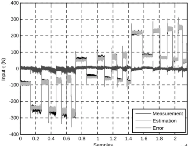
The values identified with usual IDM and OLS regressions are given in Table I and those with the new IDM in Table II. For each model, Fig. 4 and Fig. 5 present a direct validation comparing the actual τ with its predicted value Wχ . In Fig. ˆ 6, it can be seen that the variation of the usual F is the _C mean between motor and generator values, except for the 2 first masses because the load is to low and the joint works only in motor mode (see the uncertain area Fig. 3.b). That explains also why the parameter (1−α_g)m₀ is not excited enough and not well identified.

TABLE I

IDENTIFIED VALUES WITH USUAL IDM

Parameters Identified Values Standard deviation * 2 Relative deviation Ia + m0 64.799 0.477 0.4 % m0 1.047 0.012 0.6 % mae/maw 1.025 0.002 0.1 % FC 38.277 0.237 0.3 % FV 396.550 2.894 0.4 % τoff -7.935 0.078 0.5 % TABLE II

IDENTIFIED VALUES WITH NEW IDM

Parameters Identified Values Standard deviation * 2 Relative deviation (1+αm)(Ia+m0) 65.850 0.375 0.3 % (1+αm)m0 0.821 0.008 0.5 % (1+αm) 1.174 0.001 0.1 % βm 31.337 0.171 0.3 % τoffm -8.415 0.059 0.4 % (1–αg)(Ia+m0) 68.339 0.692 0.5 % (1–αg)m0 0.711 0.182 12.8 % (1–αg) 0.831 0.004 0.2 % βg 21.780 1.803 4.1 % τoffg -7.070 0.122 0.9 % FV 409.285 1.983 0.2 %

In direct validation, it is shown that the predicted torque is improved with the new IDM. It can be seen that, for the

EMPS, α_m and α_g are very close whereas β_m and β_g are significantly different. 0 0.2 0.4 0.6 0.8 1 1.2 1.4 1.6 1.8 2 x 104 -400 -300 -200 -100 0 100 200 300 400 Samples In p u t τ ( N ) Measurement Estimation Error

Fig. 4. Direct validation performed with usual IDM

0 0.2 0.4 0.6 0.8 1 1.2 1.4 1.6 1.8 2 x 104 -400 -300 -200 -100 0 100 200 300 400 Samples In p u t τ ( N ) Measurement Estimation Error

Fig. 5. Direct validation performed with new IDM.

0 50 100 150 20 25 30 35 40 45 50 55 60 Evolution of Friction Gravity - m_ag (N) F ri c ti o n ( N ) Fc (usual model) αmmag+βm αgmag+βg

Fig. 6. Evolution of Coulomb friction and comparison between the models. Moreover, Table III presents the relative norm of errors

TABLE III

RELATIVE NORM OF ERRORS WITH BOTH MODELS

Measurements used for the identification

Relative norm of errors with the usual model

Relative norm of errors with the new model

Samples without additional mass and samples with the additional masses of 1.05 kg and 3.0266 kg

0.0916 0.0908 All samples (without and with

each additional mass) 0.09996 0.0679 Table III shows that the new model does not improve the residual if the load variation is too small. Indeed, in this case (additional mass less than 3 kg), the joint runs mostly in motor behaviour, and the usual model is then sufficient. For additional mass greater than 5 kg, the load variation is large enough to justify the use of the proposed model: one observes a decrease of 30% in the relative norm of errors.

VI. DISCUSSION

The new IDM with a load-dependent joint friction model brings a substantial improvement for joint whose load can vary significantly. Robots carrying important masses or with large variation of inertial and gravity forces are considered. Moreover, the identification process is the same for both usual and new models, because the new model remains linear in relation to the parameters.

The main difficulty is to distinguish the different behaviours, motor and generator, but a solution has been proposed along this paper. However, the measurements have to be more exciting than usual. Each test has to be done with different loads to highlight the effect on the friction variations. So, this identification protocol is more time-consuming and the setting up must be adapted for the measurements with additional masses. Moreover, for robots with small load variation, the joint actuates only in one quadrant: the parameters α_m and α_g of the new model are not excited enough and the results are not better than with the usual. Then, this one will be accurate enough for low load variation.

One has to consider the load variation rate and the type of the transmission to choose the appropriate model, before starting modeling and identification.

VII. CONCLUSION

This paper has presented a new model of friction depending on load and the process to automatically identify the parameters. This technique was successfully applied on a 1 degree of freedom (dof) prismatic joint robot. From these experiments, it comes that the proposed model is accurate and useful for robots with large load variation.

Future works concern the use of this IDM to find friction parameters for a multi dof robot. The application of the model for different types of transmissions will be also studied to determine the minimum load variation rate where the new IDM is needed. The 3 load-dependent models will

be examined as well. A comparison of the method with non-linear identification will be considered. Once a load-dependent model will be identified for multi-DOF robots, it will be used for torques monitoring and collision detection.

REFERENCES

[1] C. G. Atkeson, C. H. An, and J. M. Hollerbach, “Estimation of Inertial Parameters of Manipulator Loads and Links”, in Int. J. of

Robotics Research, vol. 5(3), 1986, pp. 101-119

[2] J. Swevers, C. Ganseman, D. B. Tückel, J. D. de Schutter, and H. Van Brussel, “Optimal Robot excitation and Identification”, IEEE Trans.

on Robotics and Automation, vol. 13(5), 1997, pp. 730-740

[3] P. K. Khosla and T. Kanade, “Parameter Identification of Robot Dynamics”, in Proc. 24th _{IEEE Conf. on Decision Control,}

Fort-Lauderdale, December 1985

[4] M. Prüfer, C. Schmidt, and F. Wahl, “Identification of Robot Dynamics with Differential and Integral Models: A Comparison”, in

Proc. 1994 IEEE Int. Conf. on Robotics and Automation, San Diego,

California, USA, May 1994, pp. 340-345

[5] B. Raucent, G. Bastin, G. Campion, J. C. Samin, and P. Y. Willems, “Identification of Barycentric Parameters of Robotic Manipulators from External Measurements”, Automatica, vol. 28(5), 1992, pp. 1011-1016

[6] M. Gautier, “Identification of robot dynamics”, in Proc. IFAC Symp.

On Theory of Robots, Vienna, Austria, December 1986, pp. 351-356

[7] M. Gautier, “Dynamic identification of robots with power model”, in

Proc. IEEE Int. Conf. on Robotics and Automation, Albuquerque,

1997, pp. 1922-1927

[8] M. Gautier and P. H. Poignet, “Extended Kalman filtering and weighted least squares dynamic identification of robot”, Control

Engineering Practice, 2001

[9] W. Khalil, M. Gautier, and P. Lemoine, “Identification of the payload inertial parameters of industrial manipulators”, IEEE Int. Conf. on

Robotics and Automation, Roma, Italia, April 2007, pp. 4943-4948

[10] H.Kawasaki and K. Nishimura, “Terminal-link parameter estimation and trajectory control of robotic manipulators”, IEEE J. of Robotics

and Automation, vol. RA-4(5), pp. 485-490, 1988

[11] W. Khalil and E. Dombre, Modeling, identification and control of

robots. Hermes Penton, London, 2002

[12] M. Gautier and W. Khalil, “Direct calculation of minimum set of inertial parameters of serial robots”, IEEE Trans. on Robotics and

Automation, vol. RA-6(3), 1990, pp. 368-373

[13] M. Gautier, “Numerical calculation of the base inertial parameters”, J.

of Robotic Systems, vol. 8(4), August 1991, pp. 485-506

[14] P. P. Restrepo and M. Gautier, “Calibration of drive chain of robot joints”, in Proc. 4th _{IEEE Conf. on Control Applications, Albany,}

1995, pp. 526-531

[15] A. Gogoussis and M. Donath, “Determining the effects of Coulomb friction on the dynamics of bearings and transmissions in robot mechanisms”, J. of Mechanical Design, vol. 115, June 1993, pp. 231-240

[16] M. E. Dohring, E. Lee, and W. S. Newman, “A load-dependent transmission friction model: theory and experiments”, in Proc. IEEE

Int. Conf. on Robotics and Automation, Atlanta, Georgia, May 1993,

vol. 3, pp. 430-436

[17] C. Pelchen, C. Schweiger, and M. Otter, “Modeling and simulation the efficiency of gearboxes and of planetary gearboxes”, in Proc. 2nd

International Modelica Conference, Oberpfaffenhofen, Germany,

March 2002, pp. 257-266

[18] N. Chaillet, G. Abba, and E. Ostertag, “Double dynamic modelling and computed-torque control of a biped robot”, in Proc. IEEE/RSJ/GI

Int. Conf. on Intelligent Robots and Systems, 'Advanced Robotics Systems and the Real Word', Munich, Germany, September 1994, vol.

2, pp. 1149-1155

[19] P. Garrec, J.-P. Friconneau, Y. Measson, and Y. Perrot, “ABLE, an Innovative Transparent Exoskeleton for the Upper-Limb”, IEEE Int.

Conf. on Intelligent Robots and Systems, Nice, France, September

2008, pp. 1483-1488

[20] DSpace website, http://www.dspace.com/ww/en/pub/start.cfm [21] Mathworks website, http://www.mathworks.com/