Shaking Force Minimization of High-Speed Robots via Centre of Mass Acceleration Control

HAL Id: hal-00709167

https://hal.archives-ouvertes.fr/hal-00709167

Submitted on 25 Jun 2019

HAL is a multi-disciplinary open access archive for the deposit and dissemination of sci-entific research documents, whether they are pub-lished or not. The documents may come from teaching and research institutions in France or abroad, or from public or private research centers.

L’archive ouverte pluridisciplinaire HAL, est destinée au dépôt et à la diffusion de documents scientifiques de niveau recherche, publiés ou non, émanant des établissements d’enseignement et de recherche français ou étrangers, des laboratoires publics ou privés.

Shaking Force Minimization of High-Speed Robots via

Centre of Mass Acceleration Control

Sébastien Briot, Vigen Arakelian, Jean-Paul Le Baron

To cite this version:

Sébastien Briot, Vigen Arakelian, Jean-Paul Le Baron. Shaking Force Minimization of High-Speed Robots via Centre of Mass Acceleration Control. Mechanism and Machine Theory, Elsevier, 2012, 57, pp.1-12. �hal-00709167�

Shaking Force Minimization of High-Speed Robots

via Centre of Mass Acceleration Control

Sébastien Briot1, Vigen Arakelian2 and Jean-Paul Le Baron2

1

Institut de Recherches en Communications et Cybernétique de Nantes (IRCCyN), Nantes, France

(corresponding author) IRCCyN, Bureau 416, 1 rue de la Noë, BP 92101, F-44321 Nantes Cedex 03 FRANCE Sebastien.Briot@irccyn.ec-nantes.fr Phone : + 33 (0)2 40 37 69 58 Fax: + 33 (0)2 40 37 69 30 2

Institut National des Sciences Appliquées (INSA), Rennes, FRANCE

vigen.arakelyan@insa-rennes.fr jean-paul.le-baron@insa-rennes.fr

Abstract.

This paper deals with the problem of shaking force balancing of high-speed manipulators. The known solutions of this problem are carried out by an optimal redistribution of moving masses which allows the cancellation or the reduction of the variable loads on the manipulator frame. In this paper an innovative solution is developed which is based on the optimal control of the robot links centre of masses. Such a solution allows the reduction of the acceleration of the total mass centre of moving links and, consequently, the considerable reduction in the shaking forces. The efficiency of the suggested method is illustrated by the numerical simulations carried out for different trajectories: for examined planar two and three links serial manipulators the shaking force reduction reaches up to 77%. This approach is also a more appealing alternative to conventional balancing methods because it allows the reduction of the shaking force without counterweights. As a result, the input torques are also decreased, which is shown using dynamic simulation software.

Keywords: Shaking force, balancing, high-speed robots, optimal motion planning.

1 Introduction

A mechanical system with unbalance shaking force/moment transmits substantial vibration to the frame. Thus, a primary objective of the balancing is to cancel or reduce the variable dynamic loads transmitted to the frame and surrounding structures. Different approaches and solutions devoted to this problem have been developed and documented for one degree of freedom mechanisms [1], [2]. A new field for their applications is the design of mechanical systems for fast manipulation, which is a typical problem in advanced robotics.

The balancing of a mechanism is generally carried out by two steps: (i) the cancellation (or reduction) of the shaking force and (ii) the cancellation (or reduction) of the shaking moment. Traditionally, the cancellation of the shaking force transmitted to the manipulator frame can be achieved via adding counterweights in order to keep the total centre of mass of moving links stationary [1], via additional structures [1], [3] or by elastic components [4].

With regard to the shaking moment balancing of manipulators, the following approaches were developed: (i) balancing by counter-rotations [5]–[9], (ii) balancing by adding four-bar linkages [10]–[12], (iii) balancing by creating redundant mechanism which generates optimal trajectories of moving links [13]–[15] (vi) balancing by prescribed rotation of the end-effector [16]–[18] and (vii) balancing by adding an inertia flywheel rotating with a prescribed angular velocity [19], [20].

In the present paper we consider a simple and effective balancing method, which allows the considerable reduction of the shaking force of non-redundant manipulators without adding counterweights. It is based on the optimal control of the acceleration of the total mass centre of moving links. To the best of the authors’ knowledge, this problem is addressed for the first time.

2 Minimization of the Shaking Forces via an Optimal Motion Planning of the Total Mass Centre of Moving Links

2.1. Definition of the optimal trajectory

The shaking forces fsh of a manipulator can be written in the form: sh

i S m





f x (1)

where



m_i is the total mass of the moving links of the manipulator and x_S is the acceleration of the total mass centre. The classical balancing approach consists in adding counterweights in order to keep the total mass centre of moving links stationary. In this case, x_S= 0 for any configuration of the mechanical system. But, as a consequence, the total mass of the manipulator is considerably increased. Thus, in order to avoid this drawback, in the present study, a new approach is proposed, which consists of the optimal control of the total mass centre of moving links. Such an optimal motion planning allows the reduction of the total mass centre acceleration and, consequently, the reduction of the shaking force.

Classically, manipulator displacements are defined considering either articular coordinates q or Cartesian variables x. Knowing the initial and final manipulator configurations at time t0 and

tf, denoted as q0 = q(t0) and qf = q(tf), or x0 = x(t0) and xf = x(tf) , in the case of the control of the

Cartesian variables, the classical displacement law may be written in the form:





( )t s tq( ) f  0  0 q q q q (2a) or





( )t s t_x( ) _f  ₀  ₀ x x x x (2b)

where sq(t) and sx(t) may be polynomial (of orders 3, 5 and higher), sinusoidal, bang-bang, etc.

motion profiles [21].

From expression (1), we can see that the shaking force, in terms of norm, is minimized if the norm x_S of the masses centre acceleration is minimized along the trajectory. This means that if the displacement xS of the manipulator centre of masses is optimally controlled, the shaking

force will be minimized. As a result, the first problem is to define the optimal trajectory for the displacement xS of the manipulator centre of masses.

For this purpose, let us consider the displacement xS of a point S in the Cartesian space. First,

in order to minimize the masses centre acceleration, the length of the path followed by S should be minimized, i.e. point S should move along a straight line passing through its initial and final positions, denoted as xS0 and xSf, respectively.

Then, the motion profile used on this path should be optimized. It is assumed that, at any moment during the displacement, the norm of the maximal admissible acceleration the point S can reach is constant and denoted as x_Smax. Taking this maximal value for the acceleration into consideration, it is known that the motion profile that minimize the time interval (t0, tf) for going

from position xS0 = xS(t0) to position xSf = xS(tf) is the “bang-bang” profile [21], given by (Fig.

1a) ( ) ( ) ( ) ( ) ( ) ( ) ( ) ( ) ( ) S S S S S S S S S S t s t t s t t s t      _{ }   _{ }  f 0 0 f 0 f 0 x x x x x x x x x x (3) with max 0 max 0 ( ) / 2 1 ( ) ( ) / 2 S f S S S f x for t t t s t x for t t t      _  _   f 0 x x (4)

(a) “Bang-bang” profile (b) Trapezoidal profile

Consequently, if the time interval (t0, tf) for the displacement between positions xS0 and xSf is

fixed, the “bang-bang” profile is the trajectory that minimizes the value of the maximal acceleration x_Smax. Thus, in order to minimize x_S for a displacement during the fixed time interval (t0, tf), the “bang-bang” profile has to be applied on the displacement xS on the

manipulator total mass centre.

2.2. Observations about the modification of the optimal trajectory for taking into account the actuators properties

It should be mentioned that the given “bang-bang” profile (Fig. 1a) is based on theoretical considerations. In reality, the actuators are unable to achieve discontinuous efforts. Therefore, this motion profile should be modified by a trapezoidal profile (Fig. 1b) in order to take into account the actuators properties in terms of maximal admissible effort variations.

For a given time interval (t0, tf), the trapezoidal profile, as we define it, is characterized by

two parameters: t1, t2 (Fig. 1b). In order to find the optimal values for t1 and t2, the following

problem should be considered:

1 2 max , min S t t x  (5)

under the constraints

 

_max max i i d dt  _  (6)

where i is the input effort of the actuator i and

 

i _max the maximal admissible input effort

variation for the actuator i. This problem is highly non linear, therefore it can be solved by numerical optimization methods. It should be mentioned that in the illustrative examples given in section 3, the trapezoidal profile taking into account the actuators properties has been found using the optimisation function “fgoalattain” of Matlab.

2.3. Expression of the manipulator coordinates as a function of the mass centre parameters Once the displacement of the manipulator centre of masses is defined, the second problem is to find the articular (or Cartesian) coordinates corresponding to this displacement. For this purpose, let us consider a manipulator composed of n links. The mass of the link i is denoted as mi (i = 1, …, n) and the position of its centre of masses as xSi. Once the articular coordinates q

or Cartesian variables x are known, the values of xSi may easily be obtained using the

manipulator kinematics relationships. As a result, the position of the manipulator centre of masses, defined as 1 1 n S i Si i tot m m  



x x , where 1 n tot i i m m  



(7)

may be expressed as a function of x or q. But, in order to control the manipulator, the inverse problem should be solved, i.e. it is necessary to express variables q or x as a function of xS.

(i) dim(xS) = dim(q), i.e. the manipulator has got as many actuators as controlled variables

for the displacements xS of the centre of masses (two variables for planar cases, three

variables for spatial problems). In such case, the variables q or x can be directly expressed as a function of xS using (7), i.e. q = f(xS).

(ii) dim(xS) < dim(q), i.e. the manipulator has got more actuators than controlled variables. In

such case, the problem is under-determined as there are more parameters in variables q or

x than in xS. In order to solve it, let us consider that p0 parameters of vector q0 (or x0) and pf parameters of vector qf (or xf) are fixed. In a first task, it is necessary to define the m–p0

and m–pf other parameters of the initial and final manipulator configurations (m =

dim(q)). The way to fix it is to find the manipulator initial and final configurations, taking into account the p0 initial and pf final fixed parameters, that will allow minimizing the

norm of the vector x_Sf x_S0, i.e. the length of the displacement of the manipulator centre of masses. Then, the second task is to choose m–k articular variables among the m possible of vector q (k = dim(xS)). These m–k variables, denoted as qm–k will be controlled using some classical displacement law given at (2) or can be used in order to minimize some other performance criteria, such as the shaking moments or some other interesting performance criterion (see section 3.2). The k other variables, denoted as qk, should be expressed as a function of xS and qm–k using (7), i.e. qk = f(xS, qm–k).

In order to demonstrate the proposed balancing method, two illustrative examples are given in the following section.

3. Illustrative examples

3.1. The planar 2R serial manipulator

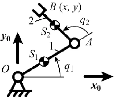
Let us consider the shaking force minimization of a 2R serial manipulator (Fig. 2). This manipulator is controlled using two rotary actuators having two input parameters which are denoted as q1 and q2. For simulations the following parameters have been used:

- lOA = 0.5 m, lAB = 0.3 m, where lOA and lAB are the lengths of segments OA and AB,

respectively;

- r1 = 0.289, where lOS1 = r1 lOA and r2 = 0.098, where lAS2 = r2 lAB, lOS1 and lAS2 being the

lengths of segments OS1 and AS2, respectively.

The mass and inertia parameters are:

- m1 = 24.4 kg and m2 = 8.3 kg, where mi is the mass of element i (i = 1, 2);

- mtool = 5 kg, where mtool is the payload;

- I1 = 1.246 kg.m² and I2 = 0.057 kg.m², where Ii is the axial moment of inertia of

element i.

Let us now express the articulated joint positions q = [q1, q2]T as a function of the position xS

of the manipulator centre of masses. From (7), we obtain:

1 1 1 2 1 1 2 2 1 1 1 2 1 1 2 1 1 2

cos cos cos( )

sin sin sin( )

cos cos( ) ... sin sin( ) S OA S OA AB S tot tot tool OA AB tot x m r l q m q q q l r l y m q m q q q q q q m l l q q q m            _{ } _{ } _{  } _{ }                   _{  } _{ }        x (8)

This relationship leads to:

2 2 2

1 1 1 1 2

(x_S l_eq cosq ) (y_S l_eq sinq ) l_eq 0 (9) where l_eq1(m r_{1 1}m₂m_tool)l_OA/m_tot and l_eq2(m r_{2 2}m_tool)l_AB/m_tot.

Replacing cos q1 and sin q1 by (1t₁2) /(1t₁2) and 2 /(1t₁ t₁2)(t1 = tan(q1/2)), respectively,

and developing (9), we obtain:

2 2 2 1 1 2 tan b b c a q c a        _ _    (10) where 1 2 _{eq S} a  l x , b 2l_eq1y_S and c xS2 yS2 leq21 leq22. (11) In (10), the sign ± stands for the two possible working modes of the manipulator (for simulations, the working mode with the “+” sign is used). Once q1 is known, q2 may easily be

found from (8): 1 1 1 2 1 1 1 sin tan cos S eq S eq y l q q q x l q      _ _    . (12)

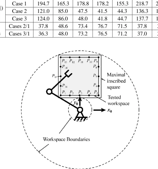
Let us now test the proposed approach. In order to show the efficiency of this optimal planning, several trajectories are tested. These trajectories are defined as follows. First, the maximal inscribed square inside of the workspace is found (Fig. 3). For this manipulator, it is a square of length 0.55 m, of which centre E is located at x = 0 m and y = 0.475 m. Then, in order to avoid problems due to the proximity of singular configuration, the tested zone is restricted to a square centred in E of edge length equal to 0.45 m (in grey on Fig. 3). Finally, we discretize each edge into four segments delimited by the points Pi (i = 1 to 16). The tested trajectories will

be the segments P1P13, P2P12, P3P11, P4P10, P5P9, P15P7, P14P8 and P13P9. Each trajectory will

have duration of 0.5 s and, for each trajectory, three different kinds of motion profiles are applied:

1. a fifth order polynomial profile is applied on the displacement of the manipulator end-effector;

2. a “bang-bang” profile is applied on the displacement of the manipulator centre of masses; 3. a trapezoidal acceleration variation is applied on the displacement of the manipulator centre of masses, taking into account that, for each actuator, the input effort variation is limited by 3.104 Nm/s.

Table 1. Maximal value of the shaking force norm for the tested trajectories of the 2R serial

manipulator. Followed path P1P13 P2P12 P3P11 P4P10 P5P9 P15P7 P14P8 P13P9 max(||fsh||) (N) Case 1 194.7 165.3 178.8 178.2 155.3 218.7 201.3 195.4 Case 2 121.0 85.0 47.5 41.5 44.3 136.3 121.7 111.8 Case 3 124.0 86.0 48.0 41.8 44.7 137.7 123.2 113.1 % of reduction Cases 2/1 37.8 48.6 73.4 76.7 71.5 37.8 39.5 42.8 Cases 3/1 36.3 48.0 73.2 76.5 71.2 37.0 38.9 42.1

(a) (b)

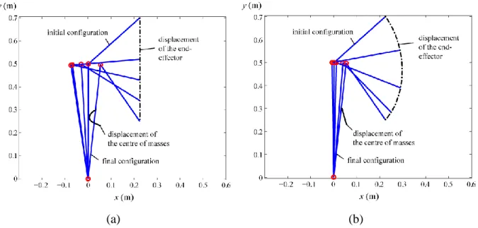
Figure 4. Manipulator end-effector displacements along the trajectory P5P9:(a) for case 1 and

(b) for cases 2 and 3.

Figure 5. Variations of the shaking forces in the case of the trajectory P5P9: case 1 (black full

line), case 2 (black dashed line) and case 3 (grey full line).

The displacements of the end-effector and manipulator links centre of masses for the trajectory P5P9 are shown in Fig. 4. These trajectory parameters are implemented into ADAMS

software and it is computed the variations of shaking forces. Fig. 5 presents the shaking force transmitted by the manipulator for trajectory P5P9. The obtained results for the whole paths are

summarized in table 1. It is shown that the optimal trajectory planning (“bang-bang profile”) allows the reduction of the shaking force from 36% up to 76.7 %. Moreover, it appears that for given actuator parameters, the minimizations obtained in the cases of the “bang-bang” and trapezoidal profiles are very close (less than 1 %). It is due to the fact that the actuators can apply high input effort variations during a displacement. However, such a result depends on the actuator power capacity and it will be variable for each type of actuator.

Obviously, the rate of reduction depends on the design parameters of the robot. For each system, it will be different

3.2. The planar 3R serial manipulator

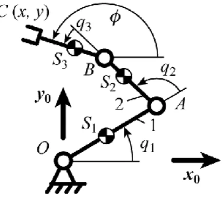
This manipulator is controlled using three rotary actuators (Fig. 6), with three input parameters which are denoted as q1, q2 and q3. The link parameters are the following:

- lOA = 0.5 m, lAB = 0.3 m, lBC = 0.1 m, where lOA, lAB and lBC are the lengths of segments OA , AB and BC, respectively;

- r1 = 0.289, where lOS1 = r1 lOA, r2 = 0.098, where lAS2 = r2 lAB, and r3 = 0.5, where lBS3 = r3 , lBC, lOS1, lAS2 and lBS3 being the lengths of segments OS1, AS2 and BS3, respectively.

Its mass and inertia parameters are:

- m1 = 24.4 kg, m2 = 8.3 kg and m3 = 2 kg, where mi is the mass of element i (i = 1, 2,

3);

- mtool = 5 kg, where mtool is the payload;

- I1 = 1.246 kg.m², I2 = 0.057 kg.m² and I3 = 0.025 kg.m², where Ii is the axial moment

of inertia of element i.

Figure 6. Schematics of the 3R serial manipulator.

In order to have the possibility to control the manipulator, let us express the relation between the articulated joint positions q = [q1, q2, q3]T and the position xS of the manipulator centre of

masses. From (7), we obtain:

1 1 1 2 1 1 2 2 1 1 1 2 1 1 2 3 3 1 1 2

cos cos cos( )

sin sin sin( )

cos cos( ) cos

sin sin( ) sin

S OA S OA AB S tot tot OA AB BC tot tool tot x m r l q m q q q l r l y m q m q q q q q q m l l r l q q q m m l m              _{ } _{ } _{  } _{ }                     _{  } _{ } _{ }  _{ }        x 1 1 2 1 1 2

cos cos( ) cos

sin sin( ) sin

OA AB BC q q q l l q q q              _{      }         (13) where  q₁ q₂q₃.

In (13), there are three unknowns q1, q2, q3 for two fixed parameters xS and yS. Therefore, as

mentioned in section 2, a way to solve this problem is to consider that one parameter, for example , is used to minimize some objective function. Then the expressions of q1, q2 and q3

can be found as a function of xS, yS and . In the remainder of the paper, angle  is used in order

to minimize the shaking moment msh of the robot. Obviously, if necessary, it can be replaced by another criterion, such the energy, the torques, etc.

2 2 2

3 1 1 3 1 1 2

((x_S l_eq cos ) l_eq cosq) ((y_S l_eq sin ) l_eq sinq) l_eq 0 (14) where l_eq1(m r_{1 1}m₂m₃m_tool)l_OA/m_tot, l_eq2(m r_{2 2}m₃m_tool)l_AB/m_tot and

3 ( 3 3 ) /

eq tool BC tot

l  m r m l m .

Replacing cos q1 and sin q1 by (1t₁2) /(1t₁2) and 2 /(1t₁ t₁2)(t1 = tan(q1/2)), respectively,

and developing (14), we obtain:

2 2 2 1 1 2 tan b b c a q c a        _ _    (15) where 1 3 2 _eq ( _{S eq} cos ) a  l x l  , (16a) 1 3 2 _eq ( _{S eq} sin ) b  l y l  , (16b) 2 2 2 2 3 3 1 2 ( _{S eq} cos ) ( _{S eq} sin ) _{eq eq} c x l   y l  l l . (16c)

In expression (15), the sign ± stands for the two possible working modes of the manipulator (for simulations, the working mode with the “+” sign is used). Once q1 is known, q2 and q3 may

easily be found from (13):

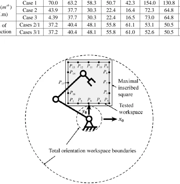
3 1 1 1 2 1 3 1 1 ( sin ) sin tan ( cos ) cos S eq eq S eq eq y l l q q q x l l q         _ _     . (17) 3 1 2 q    q q (18) Let us now test the proposed approach with this manipulator. The tested trajectories are defined as follows. First, the maximal inscribed square inside of the workspace, for any end-effector orientation, is found (Fig. 7). For this manipulator, it is a square of length 0.375 m, of which centre E is located at x = 0 m and y = 0.487 m. Then, in order to avoid problems due to the proximity of singular configuration, the tested zone is restricted to a square centred in E of edge length equal to 0.3 m (in grey on Fig. 7). Finally, we discretize each edge into four segments delimited by the points Pi (i = 1 to 16). The tested trajectories will be the segments P1P13, P2P12, P3P11, P4P10, P5P9, P15P7, P14P8 and P13P9. It should be noted that in this case

there is an independent parameter which can be defined from complementary condition describing the orientation of the end-effector. For numerical simulations, it is chosen to begin the tested trajectories with an end-effector orientation 0 = 0 deg and to finish it at f = 120 deg.

The simultaneous minimization of the shaking force and the shaking moment cannot be done without using an optimization algorithm in order to solve the following problem:

max(msh) min



 (19)

under the constraints

0 0 ( )t , ( )t_{f f}     (20a) 0 ( )t ( )t_f 0    (20b)

0 ( )t ( )t_f 0    (20c) 0 ( ) S t  S0 x x , x_S( )t_f x _Sf (20d)

Several motion profiles for  can be tested. Here it is proposed to use polynomials. Our observations showed that the polynomial function that makes it possible to obtain optimal results is of degree 8.

Each trajectory will have duration of 0.5 s and, for each trajectory three different kinds of motion profile are applied:

1. a fifth order polynomial profile is applied on the displacement (translation and rotation) of the manipulator end-effector;

2. a “bang-bang” profile is applied on the displacement of the manipulator centre of masses and the angle  is optimized in order to minimize the shaking moment;

3. a trapeze acceleration profile is applied on the displacement of the manipulator centre of masses, taking into account that, for each actuator, the input effort variation is limited by 3.104 Nm/s; the trajectory for angle  optimized in the previous case is used in order to compute the actuator displacements.

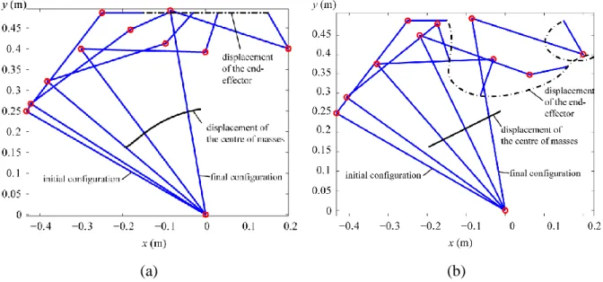
The displacements of the end-effector and manipulator links centre of masses for the trajectory P15P7 are shown in Fig. 8. Fig. 9 presents the shaking force and shaking moment for

the path P15P7. The obtained results for the whole paths are summarized in table 2 and 3. It is

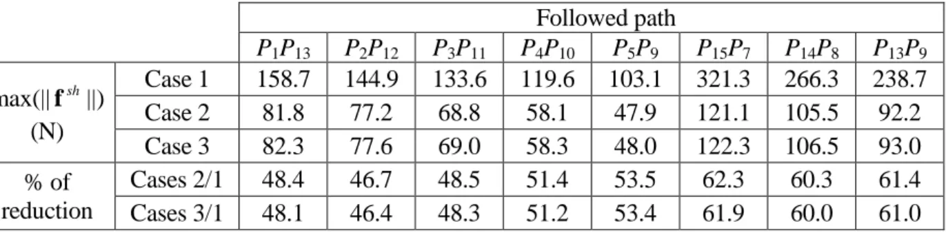
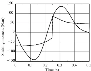
shown that the optimal trajectory planning (“bang-bang” profile) allows the reduction of the shaking forces from 48 % up to 62.2 %. Moreover, with a simultaneous optimal control of angle , the shaking moment can be reduced from 37.2 % up to 61 %.

As previously mentioned, these results depend on the design parameters of the used robot. For another manipulator, they will be different. But, in any case the shaking force and moment shall be decreased.

Table 2. Maximal value of the shaking force norm for the tested trajectories on the 3R serial

manipulator. Followed path P1P13 P2P12 P3P11 P4P10 P5P9 P15P7 P14P8 P13P9 max(|| sh||) f (N) Case 1 158.7 144.9 133.6 119.6 103.1 321.3 266.3 238.7 Case 2 81.8 77.2 68.8 58.1 47.9 121.1 105.5 92.2 Case 3 82.3 77.6 69.0 58.3 48.0 122.3 106.5 93.0 % of reduction Cases 2/1 48.4 46.7 48.5 51.4 53.5 62.3 60.3 61.4 Cases 3/1 48.1 46.4 48.3 51.2 53.4 61.9 60.0 61.0

Table 3. Maximal value of the shaking moment for the tested trajectories on the 3R serial manipulator. Followed path P1P13 P2P12 P3P11 P4P10 P5P9 P15P7 P14P8 P13P9 max(msh) (N.m) Case 1 70.0 63.2 58.3 50.7 42.3 154.0 130.8 119.6 Case 2 43.9 37.7 30.3 22.4 16.4 72.3 64.8 57.0 Case 3 4.39 37.7 30.3 22.4 16.5 73.0 64.8 52.3 % of reduction Cases 2/1 37.2 40.4 48.1 55.8 61.1 53.1 50.5 57.0 Cases 3/1 37.2 40.4 48.1 55.8 61.0 52.6 50.5 52.2

(a) (b)

Figure 8. Manipulator end-effector displacements along the trajectory P15P7:(a) for case 1 and

(b) for optimal cases 2 and 3.

Figure 9. Variations of the shaking forces in the case of the trajectory P15P7: case 1 (black full

Figure 10. Variations of the shaking moment in the case of the trajectory P15P7: case 1 (black

full line), case 2 (black dashed line) and case 3 (grey full line).

3.3. Observations about input torques

The main drawback of the shaking force balancing by counterweights is the increase of the inertia of moving links caused by adding masses, and consequently, the increase of input torques. The advantage of the suggested balancing method is in the fact that the shaking forces are only reduced by optimal control of moving links, without adding counterweights. It results in the fact that the input torques are considerably lower than in the case of balancing by counterweights. To illustrate this advantage for examined 2R serial manipulator, three kinds of simulations have been carried out using dynamic simulation software: (a) unbalanced manipulator carrying out a straight line trajectory along P5P9 (Fig. 4) using a fifth order

polynomial motion profile; (b) manipulator balanced by counterweights along the same trajectory1; (c) manipulator controlled via optimal centre of mass displacement between points P5 and P9.

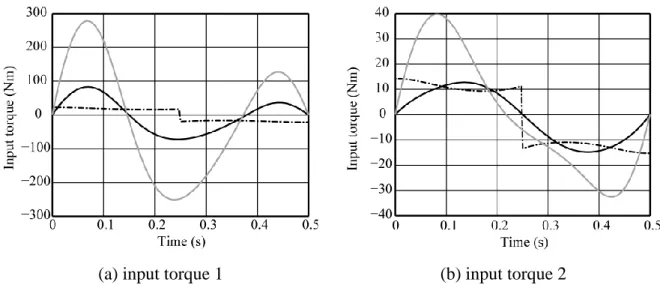
The obtained results are given in Figure 11. The software simulations showed that in comparison with mass balanced manipulator a 92% reduction in input torque is achieved, and, in comparison with unbalanced manipulator a 73% reduction in input torque is achieved.

Finally, we would like to mention that the method proposed in this paper focused exclusively on the force balancing because it is carried out by optimisation of the trajectory of the manipulator’s center of mass. However, as was shown above, it also allows the reduction of the shaking moment and the input torques. Such a result has been observed for many simulated manipulators. But it is not possible to pretend in any way that this will be true for any manipulator.

(a) input torque 1 (b) input torque 2

Figure 11. Manipulator input torques for trajectory P5P9 corresponding to the three simulated

models: (i) unbalanced manipulator carrying out a straight line trajectory of the end-effector using a fifth order polynomial motion profile (black full line); (ii) manipulator balanced by

counterweights along the same trajectory (grey full line); (iii) manipulator controlled via optimal centre of mass displacement (black dashed line).

4. Conclusions

In this paper, we have presented a new approach, based on an optimal trajectory planning, which allows the considerable reduction of the shaking force. This simple and effective balancing method is based on the optimal control of the acceleration of the manipulator centre of masses. For this purpose, the “bang-bang” profile has been used. The aim of the suggested method consists in the fact that the manipulator is controlled not by applying end-effector trajectories but by planning the displacements of the total mass centre of moving links. The trajectories of the total mass centre of moving links are defined as straight lines and are parameterized with “bang-bang” profile. Such a control approach allows the reduction of the maximum value of the centre of mass acceleration and, consequently, the reduction in the shaking force. It should be mentioned that such a solution is also very favourable for reduction of input torques because it is carried out without adding counterweights. The proposed balancing method has been illustrated via two examples. The numerical simulations showed that considerable reduction in shaking force and input torques were achieved.

References

[1] Lowen, G.G., Tepper, F.R., and Berkof, R.S. (1983). Balancing of linkages – an Update. Mechanism and Machine Theory. 18(3). 213-230.

[2] Arakelian, V, and Smith, M.R. (2005). Shaking force and shaking moment balancing of mechanisms: a historical review with new examples. Transactions of the ASME, Journal of Mechanical Design. 127. 334-339.

[3] van der Wijk, V. Herder J. L. (2012). Synthesis method for linkages with centre of mass at invariant link point — Pantograph based mechanisms. Mechanism and Machine Theory. 48. 15-28.

[4] Alici, G., and Shirinzadeh, B. (2003) Optimum force balancing with mass distribution and a single elastic element for a five-bar parallel manipulator, In Proceedings of the 2003 IEEE International Conference on Robotics and Automation, Taipei, Taiwan, Sept. 14–19, pp. 3366–3371.

[5] Berkof, R.S. (1973). Complete force and moment balancing of inline four-bar linkages. Mechanism and Machine Theory. 8(3). 397-410.

[6] Dresig, H., Naake, S., and Rockausen L. (1994). Vollständiger und harmonischer Ausgleich ebener Mechanismen.VDI Verlag, Düsseldorf, 73p.

[7] Arakelian, V, and Smith, M.R. (1999). Complete shaking force and shaking moment balancing of linkages. Mechanism and Machine Theory. 34(8). 1141-1153.

[8] Herder, J.L., and Gosselin, C.M. (2004). A counter-rotary counterweight for light-weight dynamic balancing. In Proceedings of ASME 2004 DETC/CIEC Conference, September 28 – October 2, Salt Lake City, Utah, USA. 659-667.

[9] van der Wijk, Demeulenaere, B., Gosselin, C., V. Herder J. L. (2012). Comparative analysis for low-mass and low-inertia dynamic balancing of mechanisms. Transactions of the ASME, Journal of Mechanisms and Robotics. 4. 031008 / 1-8.

[10] Ricard, R., and Gosselin, C.M. (2000). On the design of reactionless parallel manipulators. In Proceedings of the ASME 2000 DETC/CIEC Conference, Baltimore, Maryland, September 10-13. 1-12.

[11] Gosselin, C.M., Cote, G., and Wu, Y. (2004). Synthesis and design of reactionless tree-degree-of-freedom parallel mechanisms. IEEE Transactions on Robotics and Automation. 20(2). 191-199.

[12] Jiang Q., Gosselin, G.M. (2010). Dynamic optimization of reactionless four-bar linkages. Transactions of the ASME, Journal of Dynamic Systems, Measurement, and Control. 132. 041006 / 1-11.

[13] Papadopoulos, E., and Abu-Abed, A. (1994). Design and motion planning for a zero-reaction manipulator. In Proceedings of the IEEE International Conference on Robotics and Automation, San Diego, CA. 1554-1559.

[14] He G. and Lu Z. (2006). Optimal motion planning of parallel redundant Mechanisms woth Shaking Force Reduction. In Proceedings of the IMACS conference, October 4-6, 2006, Beijing, China, 1132-1139.

[15] Nenchev, D., Yoshida, K., Vichitkulsawat, P. and Uchiyama, M. (1999) Reaction null-space control of flexible structure mounted manipulator systems. IEEE Transactions on Robotics and Automation, 15(6). 1011-1023.

[16] Fattah, A., and Agrawal, S.K. (2006). On the design of reactionless 3-DOF planar parallel mechanisms. Mechanism and Machine Theory. 41(1). 70-82.

[17] Arakelian, V., and Briot, S. (2008). Dynamic balancing of the SCARA robot. In Proceedings of the 17th CISM-IFToMM Symposium on Robot Design, Dynamics, and Control (Romansy 2008), Tokyo, Japan, July 5-9.

[18] Briot, S., and Arakelian, V. (2009). Complete shaking force and shaking moment balancing of the position-orientation decoupled PAMINSA manipulator », IEEE/ ASME International Conference on Advanced Intelligent Mechatronics (AIM2009), July 14-17, Singapore.

[19] Arakelian, V. and Smith, M.R. (2008). Design of planar 3-DOF 3-RRR reactionless parallel manipulators. Mechatronics, 18, 601-606.

[20] van der Wijk, V. and Herder, J.L. (2010). Active dynamic balancing unit for controlled shaking force and shaking moment balancing. Proceedings of the the ASME 2010 International Design Engineering Technical Conferences & Computers and Information in Engineering Conference (IDETC/CIE 2010), August 15-18, Montreal, Quebec, Canada.

[21] Khalil, W., and Dombre, E. (2002). Modeling, identification and control of robots. Hermes Sciences Europe.

Figures captions

Figure 1. Motion profiles used for the shaking force minimization. Figure 2. Schematics of the 2R serial manipulator.

Figure 3. The tested trajectories of the 2R serial manipulator.

Figure 4. Manipulator end-effector displacements along the trajectory P5P9:(a) for case 1 and

(b) for cases 2 and 3.

Figure 5. Variations of the shaking forces in the case of the trajectory P5P9: case 1 (black full

line), case 2 (black dashed line) and case 3 (grey full line).

Figure 6. Schematics of the 3R serial manipulator.

Figure 7. The tested trajectories of the 3R serial manipulator.

Figure 8. Manipulator end-effector displacements along the trajectory P15P7:(a) for case 1 and

(b) for optimal cases 2 and 3.

Figure 9. Variations of the shaking forces in the case of the trajectory P15P7: case 1 (black full

line), case 2 (black dashed line) and case 3 (grey full line).

Figure 10. Variations of the shaking moment in the case of the trajectory P15P7: case 1 (black

full line), case 2 (black dashed line) and case 3 (grey full line).

Figure 11. Manipulator input torques for trajectory P5P9 corresponding to the three simulated

models: (i) unbalanced manipulator carrying out a straight line trajectory of the end-effector using a fifth order polynomial motion profile (black full line); (ii) manipulator balanced by counterweights along the same trajectory (grey full line); (iii) manipulator controlled via optimal centre of mass displacement (black dashed line).

Tables captions

Table 1. Maximal value of the shaking force norm for the tested trajectories of the 2R serial

manipulator.

Table 2. Maximal value of the shaking force norm for the tested trajectories on the 3R serial

manipulator.

Table 3. Maximal value of the shaking moment for the tested trajectories on the 3R serial