Parallel and Multistep Simulation of Power System Transients

(1)

affiliée à l’Université de Montréal

Parallel and multistep simulation of power system transients

MING CAI

Département de génie électrique

Thèse présentée en vue de l’obtention du diplôme de Philosophiæ Doctor Génie électrique

Octobre 2019

(2)

affiliée à l’Université de Montréal

Cette thèse intitulée :

Parallel and multistep simulation of power system transients

présentée par Ming CAI

en vue de l’obtention du diplôme de Philosophiæ Doctor a été dûment acceptée par le jury d’examen constitué de :

Keyhan SHESHYEKANI, président

Jean MAHSEREDJIAN, membre et directeur de recherche Ilhan KOCAR, membre et codirecteur de recherche

Houshang KARIMI, membre

(3)

DEDICATION

(4)

ACKNOWLEDGEMENTS

First and foremost, I would like to express my sincere gratitude to Dr. Jean Mahseredjian, my Ph.D. director, for the opportunity he gave me to study at Polytechnique Montréal, as well as his patience, advice and continuous support during the entire four years of my research. His work ethic and comprehensive knowledge have greatly inspired and motivated me in my future career orientation. I also owe my gratitude to Dr. Akihiro Ametani for his constant support, advice, encouragement, and all the discussions we have had. Time spent with him has been a great joy in both my professional and personal life.

I would like to thank Mr. Ali El-Akoum from Électricité de France (EDF) Lab Paris-Saclay and Mr. Emmanuel Rutovic for the valuable discussions on the Functional Mock-up Interface (FMI) standard.

Guidance, advice and help from Mr. Aboutaleb Haddadi are much appreciated.

Special thanks to all my colleagues, those who have already left and who will continue, for their friendship and support: Isabel Lafaia, Baki Cetindag, Louis Filliot, Xiaopeng Fu, Fidji Diboune, Serigne Seye, Thomas Kauffmann, Haoyan Xue, Anas Abusalah, Jesus Morales, Miguel Martinez, Anton Stepanoz, Diane Desjardins, Reza Hassani, Masashi Natsui, David Tobar, Nazak Soleimanpour, Willy Mimbe, and Aramis Trevisan. It was a great pleasure to have worked with you.

Last but not least, to my parents who have always been there for me, I have no words but my ultimate love and appreciation.

(5)

RÉSUMÉ

La simulation des régimes transitoires électromagnétiques (EMT) est devenue indispensable aux ingénieurs dans de nombreuses études des réseaux électriques. L’approche EMT a une nature de large bande et est applicable aux études des transitoires lents (électromécaniques) et rapides (électromagnétiques). Cependant, la complexité des reseaux électriques modernes qui ne cesse de s’accroître, particulièrement des réseaux avec des interconnexions HVDC et des éoliennes, augmente considérablement le temps de résolution dans les études des transitoires électromagnétiques qui exigent la résolution précise des systèmes d’équations différentielles et algébriques avec un pas de calcul pré-déterminé. En tant que sujet de recherche, la réduction du temps de résolution des grands réseaux électriques complexes a donc attiré beaucoup d’attention et d’intérêt. Cette thèse a pour objectif de proposer de nouvelles méthodes numériques qui sont efficaces, flexibles et précises pour la simulation des régimes transitoires électromagnétiques des réseaux électriques.

Dans un premier temps, une approche parallèle et à pas multiples basée sur la norme Functional

Mock-up Interface (FMI) pour la simulation transitoire des réseaux électriques avec systèmes de

contrôle complexes est développée. La forme de co-simulation de la norme FMI dont l’objectif est de faciliter l’échange de données entre des modèles développés avec différents logiciels est implémentée dans EMTP. Tout en profitant de cette implémentation, les différents systèmes de contrôle complexes peuvent être découplés du réseau principal en mémoire et résolus de façon indépendante sur des processeurs séparés. Ils communiquent avec le reseau principal à travers une interface de co-simulation pendant une simulation. Cette méthodologie non seulement réduit la charge de calcul total sur un seul processeur, mais elle permet aussi de simuler les systèmes de contrôle découplés de façon parallèle et à pas multiples. Deux modes de co-simulation sont proposés dans la première étape du développement, qui sont les modes asynchrone et synchrone. Dans le mode asynchrone, tous les systèmes de contrôle découplés (esclaves) sont simulés en parallèle avec le réseau principal (maître) en utilisant un seul pas de calcul tandis que le mode synchrone permet une simulation séquentielle en utilisant différents pas de calcul dans le maître et les esclaves. La communication entre le maître et les esclaves est realisée et coordonée par des fonctions qui implémentent le primitif de synchronisation de bas niveau sémaphore. Dans la deuxième étape du développement, afin d’améliorer la méthodologie originale, un nouveau mode asynchrone parallèle à pas multiples (parallel multistep asynchronous mode) et une procédure de

(6)

correction de signaux sont proposés. Le premier combine les avantages numériques (respectivement la simulation en parallèle et à pas multiples) des deux modes développés précédemment et la seconde, basée sur l’extrapolation linéaire, sert à améliorer la précision de simulation. Cette approche est testée sur différents benchmarks des réseaux électriques avec systèmes de contrôle complexes tels que les contrôles éoliens et les relais de protection. Ses avantages de pouvoir entretenir et améliorer la précision, accélérer la simulation temporelle tout en étant évolutive et flexible sont démontrés par les résultats de simulation en comparaison avec ceux obtenus des simulations EMT sur un seul processeur.

Dans un deuxième temps, une approche de parallélisation-dans-le-temps (parallel-in-time) basée sur la technique parallèle de regroupement et permutation d’équations (equation grouping and

reordering technique, PEGR) pour la simulation transitoire des réseaux électriques est développée

dans la thèse. La proposition originale de la technique PEGR, formulée dans une forme d’état, a pour objectif de réduire le nombre total de pas de calcul de façon logarithmique en regroupant et permutant les équations du réseau à plusieurs points de calcul. L’approche de parallélisation-dans-le-temps développée dans cette thèse est adaptée à l’analyse nodale modifiée augmentée

(modified-augmented-nodal analysis, MANA). Elle est implémentée en C++ avec l’API OpenMP

Multithreading pour la parallélisation de résolution en utilisant différents nombres de fils. Le solveur linéaire hautement efficace à matrice creuse KLU est utilisé comme le solveur pour les matrices de réseau. Certaines stratégies de programmation et solutions aux problèmes rencontrés dans les simulations transitoires réalistes des réseaux électriques sont inclues dans le développement de l’approche. Cette approche de parallélisation-dans-le-temps permet une formulation flexible en regroupant les équations du réseau à différents nombres de points de calcul, qui est ajustable par rapport au nombre de processeurs de l’ordinateur utilisé. Afin de valider la précision et l’efficacité de l’approche développée, elle est testée sur des benchmarks réalistes des réseaux électriques et d’autres construits avec de nombreuses répliques de ces mêmes benchmarks représentant des réseaux électriques à plus grandes échelles. Les résultats obtenus de cette approche démontrent qu’elle peut accélérer la simulation temporelle des réseaux électriques à différentes échelles en utilisant différents nombres de processeurs parallèles, en comparaison avec la méthode de résolution séquentielle traditionnelle.

(7)

ABSTRACT

The simulation of electromagnetic transients (EMT) has become indispensable to utility engineers in a multitude of studies in power systems. The EMT approach is of wideband nature and applicable to both slower electromechanical as well as faster electromagnetic transients. However, the ever-growing complexity of modern-day power systems, especially those with HVDC interconnections and wind generations, considerably increases computational time in EMT studies which require the accurate solution of usually large sets of differential and algebraic equations (DAEs) with a pre-determinded time-step. Therefore, computing time reduction for solving complex, practical and large-scale power system networks has become a hot research topic. This thesis proposes new fast, flexible and accurate numerical methods for the simulation of power system electromagnetic transients.

As a first step in this thesis, a parallel and multistep approach based on the Functional Mock-up Interface (FMI) standard for power system EMT simulations with complex control systems is developed. The co-simulation form of the FMI standard, a tool independent interface standard aiming to facilitate data exchange between dynamic models developed in different simulation environments, is implemented in EMTP. Taking advantage of the compatibility established between the FMI standard and EMTP, various computationally demanding control systems can be decoupled from the power network in memory, solved independently on separate processors, and communicate with the power network through a co-simulation interface during a simulation. This not only reduces the total computation burden on a single processor, but also allows parallel and multistep simulation for the decoupled control systems. Following a master-slave co-simulation scheme (with the master representing the power network and the slaves denoting the decoupled control systems), two co-simulation modes, which are respectively the asynchronous and synchronous modes, are proposed in the first stage of the development. In the asynchronous mode, all decoupled subsystems are simulated in parallel with a single numerical integration time-step whereas the synchronous mode allows the use of different numerical time-steps in a sequential co-simulation environment. The communication between master and slaves is coordinated by functions employing the low-level synchronization primitive semaphore. The second stage of the development improves the original methodology by proposing the parallel multistep asynchronous mode that combines the advantages (parallel and multistep simulation) of the previously developed two modes together and a linear extrapolation-based signal correction procedure for enhanced

(8)

simulation accuracy. All developments in this approach are tested on realistic power system benchmarks with complex control systems such as wind generator controls and protection relays. The advantages of this approach in maintaining and improving accuracy, simulation speedup, scalability as well as flexibility are demonstrated by simulation results in comparison to conventional single-core-based EMT simulations.

Next, a parallel-in-time approach based on the parallel-in-time equation grouping and reordering (PEGR) technique is developed in the thesis for power system EMT simulations. The original proposition of the PEGR technique aims to logathrimically reduce the number of time-domain solution steps by grouping network equations at several solution time-points together and taking advantage of independency between certain solution steps found after a series of recursive row and column reordering. The parallel-in-time approach developed in this thesis adapts the original formulation of the PEGR technique into the modified-augmented-nodal analysis (MANA) from state-space and is implemented using C++ with API OpenMP Multithreading for parallelization using different numbers of threads. The highly efficient sparse linear solver KLU is used as the network matrix solver. Several programming concerns and issues encountered in realistic power system EMT simulations are also considered in the development of this approach. This parallel-in-time approach allows flexible formulation in grouping the network equations at different numbers of solution time-points, catering to the computing capacity (in terms of the number of logical processors) of the PC used in the simulation. Realistic power system benchmarks as well as larger networks constructed with multiple replicas of these benchmarks are used to test the accuracy and efficiency of the proposed approach. Its capability of speeding up a time-domain simulation using different numbers of parallel processors for power systems of different levels of complexity is demonstrated through simulation results in comparison to the conventional stepwise solution scheme.

Finally, several possible future developments based on the completed work proposed in the thesis are presented.

(9)

LIST OF TABLES

Table 2.1 Attributes of node fmiModelDescription ... 14

Table 2.2 Attributes of node fmiModelDescription\CoSimulation ... 15

Table 2.3 Attributes of node fmiModelDescription\ModelVariable ... 16

Table 2.4 Structure of the container InOut (co-simulation bus) ... 39

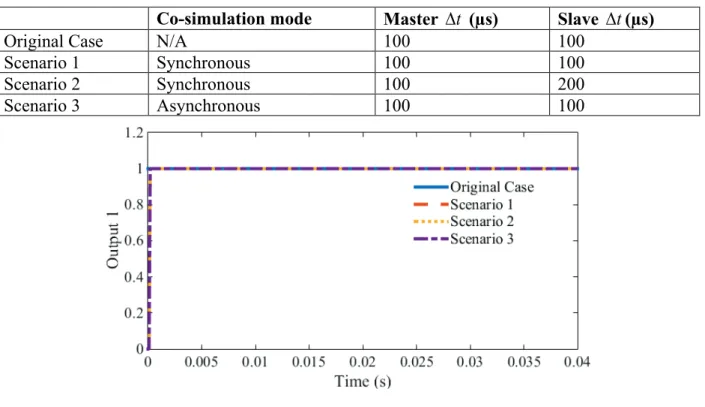
Table 3.1 Co-simulation mode scenarios, co-simulation interface design validation ... 54

Table 3.2 Co-simulation mode scenarios, accuracy validation of the original methodology, Network-1 ... 57

Table 3.3 Relay 1 to 5 tripping zones ... 66

Table 3.4 Co-simulation mode scenarios, accuracy validation of the original methodology, Network-2 ... 66

Table 3.5 Hardware and software configurations of the PCs ... 72

Table 3.6 Co-simulation mode scenarios, computation time gains ... 72

Table 3.7 Comparison of solution times (s) on a PC with 2 cores (4 logical processors) for different scenarios, Network-1 ... 73

Table 3.11 Snippet of comparison of solution times (s) on a PC with 2 cores (4 logical processors) for different scenarios, Network-2 ... 80

Table 3.12 Co-simulation mode scenarios, accuracy validation of the parallel multistep asynchronous mode ... 82

(15)

Table 3.13 Co-simulation mode scenarios, accuracy validation of the linear extrapolation-based signal correction procedure, Network-3 ... 84 Table 3.14 Co-simulation mode scenarios, accuracy validation of the linear extrapolation-based

signal correction procedure, Network-4 ... 89 Table 3.15 Co-simulation mode scenarios, computation time gains with the parallel multistep

asynchronous mode, Network-1 and -2 ... 93 Table 3.16 Comparison of solution times (s) on the PC with 16 cores for different scenarios,

Network-1, improved methodology ... 94 Table 3.17 Comparison of solution times (s) on the PC with 16 cores for different scenarios,

Network-2, improved methodology ... 95 Table 3.18 Hardware and software configurations of the 24-core PC ... 96 Table 3.19 Co-simulation mode scenarios, computation time gains with the parallel multistep

asynchronous mode, Network-4 ... 96 Table 3.20 Comparison of solution times (s) on the PC with 24 cores (48 logical processors) for

different scenarios, Network-4, improved methodology ... 97 Table 5.1 Performance timings of test case 1 ... 130 Table 5.2 Performance timings of test case 2 ... 132

(16)

LIST OF FIGURES

Figure 2.1 FMI for model exchange ... 12

Figure 2.2 FMI for co-simulation ... 13

Figure 2.3 Interfacing three subnetworks (Master, Slave 1 and Slave 2) via DLL files and two co-simulation buses ... 19

Figure 2.4 One possible implementation of the master program of co-simulation of an UML 2.0 state machine ... 27

Figure 2.5 Principal function calling sequence in the master algorithm ... 28

Figure 2.6 Principal function calling sequence in the slave algorithm ... 29

Figure 2.7 Synchronization scheme between master and slave during initialization stage ... 34

Figure 2.8 Synchronization scheme between master and slave in synchronous mode (with a single numerical integration time-step) ... 35

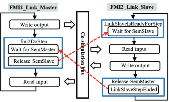
Figure 2.9 Synchronization scheme between master and slave in asynchronous mode (with a single numerical integration time-step) ... 36

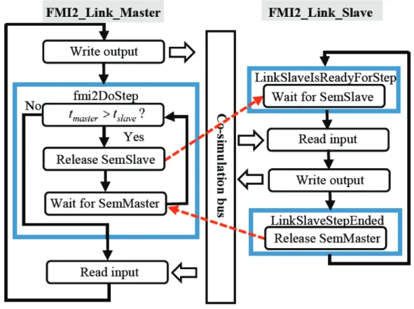
Figure 2.10 Function fmi2DoStep in synchronous mode (with different numerical integration time-steps) ... 37

Figure 2.11 Synchronization scheme between master and slave in synchronous mode ... 37

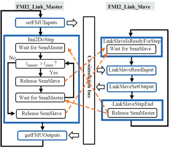
Figure 2.12 Synchronization scheme between master and slave in the improved asynchronous mode (parallel multistep asynchronous mode) ... 41

Figure 2.13 First synchronization scenario (∆t_master = ∆t_slave) between master and slave in the parallel multistep asynchronous mode ... 42

Figure 2.14 Second synchronization scenario (∆t_master < ∆t_slave) between master and slave in the parallel multistep asynchronous mode ... 43

Figure 2.15 Third synchronization scenario (∆t_master > ∆t_slave) between master and slave in the parallel multistep asynchronous mode ... 44

(17)

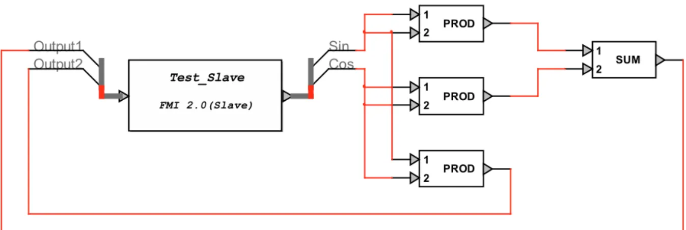
Figure 3.2 Slave subsystem for the validation of co-simulation interface design ... 50

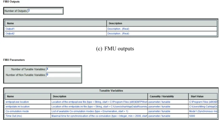
Figure 3.3 Inputs and outputs settings in the slave ... 51

Figure 3.4 Co-simulation mode and other parameter settings in the slave ... 51

Figure 3.5 Master subsystem for the validation of co-simulation interface design ... 52

Figure 3.6 Loaded data and parameters from the slave FMU in the master ... 53

Figure 3.7 Waveforms of Output 1 for all simulation scenarios ... 54

Figure 3.8 Waveforms of Output 2 for all simulation scenarios ... 55

Figure 3.9 Closer observation of waveform of Output 2 for all simulation scenarios ... 55

Figure 3.10 Network-1 benchmark ... 58

Figure 3.11 Offshore wind parks and HVDC connection in Network-1 ... 59

Figure 3.12 Design of one offshore wind park in Network-1 ... 59

Figure 3.13 DFIG model in the offshore wind parks in Network-1 ... 60

Figure 3.14 Control system design for the DFIG model in the offshore wind parks ... 60

Figure 3.15 Waveforms of average active power and phase-a current ... 61

Figure 3.16 Line relay at each end of a CP line ... 62

Figure 3.17 Relay 1 settings (partial) ... 64

Figure 3.19 Tripping instants of Relays 1, 2 and 4 ... 67

Figure 3.20 Phase a locus of Relay 1 ... 68

Figure 3.21 Simplified co-simulation process of Scenario 1 ... 69

Figure 3.22 Simplified co-simulation process of Scenario 3 ... 70

Figure 3.23 Total solution time speedup with respect to the number of slaves in Network-1 on a PC with 2 cores (4 logical processors) ... 73

(18)

Figure 3.25 Total solution time speedup with respect to the number of slaves in Network-2 on a

PC with 2 cores (4 logical processors) ... 75

Figure 3.27 Solution scheme in the original approach (EMTP) for the computation of one time-step. ... 77

Figure 3.28 Solution scheme using the FMI-based co-simulation approach (parallel asynchronous mode) for the computation of one time-step. ... 78

Figure 3.29 Tripping instants of Relays 1, 2 and 4 ... 83

Figure 3.31 Phase-b voltage at bus XFMR between t =0.5s and t=0.55s without signal correction with closer observation of waveforms in the amplified region ... 86

Figure 3.32 Phase-b voltage at bus XFMR between t =0.5s and t=0.55s with signal correction with closer observation of waveforms in the amplified region ... 87

Figure 3.34 Design of the F1 wind park feeder ... 90

Figure 3.35 DFIG model with wind generator control systems modelled using the detailed model ... 91

Figure 3.36 Control system design for the DFIG model in the wind generator ... 91

Figure 3.37 Average active power from wind park feeders ... 92

Figure 3.38 Phase-a voltage at the 34.5 kV bus ... 92

Figure 3.39 Total solution time speedup with respect to the number of slaves in Network-1 on a 16-core PC, improved methodology ... 94

(19)

Figure 4.1 Multiphase pi-section schematic ... 103 Figure 4.2 Expanded network equations incorporating current history terms into the vector of

unknowns, demonstrating interdependency of solutions at adjacent time-points ... 104 Figure 4.3 Lower triangular matrix L and equations for forward substitution after a one-time row

and column reordering and LU factorization ... 110 Figure 4.4 Lower triangular matrix L and equations for forward substitution after recursive row

and column reordering and LU factorization ... 111 Figure 4.5 : Structure of the L and U factors when grouping the network equations of 16 time-steps ... 120 Figure 4.6 Switching between the PEGR-based approach and the conventional approach in the

case of topological changes in the network ... 123 Figure 5.1 Network-5 benchmark ... 127 Figure 5.2 Phase-a fault current, phase-a voltages at buses 888 and 854 ... 128 Figure 5.3 Solution time speedup using the PEGR-based parallel-in-time approach with respect to

the number of launched threads in the simulation for test case 1 ... 130 Figure 5.4 Network-6 benchmark ... 131 Figure 5.5 Solution time speedup using the PEGR-based parallel-in-time approach with respect to

(20)

LIST OF SYMBOLS AND ABBREVIATIONS

DAE Differential and algebraic equation DLL Dynamic-link library

EMT Electromagnetic transients

EMTP Electromagnetic transients program FA Frequency adaptive

FDNE Frequency-dependent network equivalent FMI Functional Mock-up Interface

FMU Functional Mock-up Unit FPGA Field-programmable gate array GPU Graphics processing unit HVDC High voltage direct current

MANA Modified-augmented-nodal analysis

PEGR Parallel-in-time equation grouping and reordering TS Transient stability

(21)

LIST OF APPENDICES

Appendix A – Example xml file in an Functional Mock-up Unit (FMU) ... 154 Appendix B – Detailed implementation of funcitons coordinating master-slave co-simulation . 159 Appendix C – Algorithm for the extraction of block elements in the L and U factors ... 167 Appendix D – List of publications ... 172

(22)

CHAPTER 1 INTRODUCTION

1.1 Motivation

Modern-day power systems are increasingly complex, thanks to more and more challenging cases created by state-of-the-art developments in the research fields such as HVDC systems and wind generation [1]. Such ever-growing complexity of modern power grids requires high-performance computing resources (preferably inexpensive) as well as advanced computer-based simulation methods for design, operation and post-mortem analysis stages.

Numerical solution methods are crucial in the evolution and technological advancements in modern power systems, in which circuit-based numerical methods, such as those used in the high accuracy time-domain electromagnetic transients (EMT) simulations, are of particular interest to researchers and utility engineers. The EMT approach [2]-[6] targets operation problems in power system analyses. It helps utility engineers perform highly accurate studies including fault analysis, power flow analysis, stability analysis as well as EMT analysis, demonstrating great advantages over phasor-domain approaches [7], [8]. It is of wideband nature and applicable to both slower electromechanical transients of lower frequencies as well as high frequency electromagnetic transients, such as switching and lightning. Typical numerical integration time-steps are in the range of µs, which creates major obstacles in terms of computing times in the accurate solution of large sets of differential and algebraic equations (DAE) for large-scale systems. Therefore, computing time reduction for solving complex, practical and large-scale power system networks has become a hot research topic.

1.1.1 Accelerating EMT simulations—numerical solution algorithms

Over the years, many efforts have been dedicated to reducing computing times in EMT-type simulation methods, in which development of models and new numerical solution algorithms have drawn a fair amount of interest among researchers. The modelling aspect focuses mainly on enhancing computational performance and optimizing accuracy for a given numerical integration time-step in the implementation of model equations [9], [10]. Although this could, in some cases, allow the adoption of larger numerical integration time-steps to improve simulation efficiency, properly maintaining the accuracy, generalization and application in large-scale networks need to

(23)

be further investigated. Therefore, more efforts have been dedicated to the research on numerical solution algorithms for enhancing the performance of EMT-type solution schemes, which fall principally into the following categories: adoption of sparse matrix solvers, parallelization techniques, hybrid techniques, network equivalents and frequency adaptive methods.

1.1.1.1 Adoption of sparse matrix solvers

Among all the available sparse linear solvers for efficient large sparse matrix solutions, LU factorization is a popular approach and is used as a direct solver in circuit simulation [11]. In particular, a Gilbert-Peierls’ left-looking algorithm based sparse high-performance linear solver named KLU stands out in the solution of circuit matrices thanks to the efficient ordering mechanisms and high-performance factorization and solve algorithms it adopts [12], [13]. Moreover, KLU uses a hybrid ordering strategy consisting of an unsymmetrical permutation to ensure a zero-free diagonal, a symmetrical permutation to Block Triangular Form (BTF) and a fill-in reducfill-ing orderfill-ing scheme to achieve a superior fill-fill-in quality and good performance speedup when compared to other existing sparse linear solvers for circuit simulation [12], [13]. A KLU-based simulator developed in [13] has demonstrated its numerical advantages for solving circuit matrices. Other LU factorization-based software packages can be found in [11].

1.1.1.2 Parallelization techniques

Parallelization is another area that has been researched in depth in computing time reduction. Throughout the years, a great number of techniques and methods have been proposed and developed in which parallelization is achieved by partitioning a network using the intrinsic propagation delay at distributed parameter transmission line and cable models for natural decoupling of networks while adopting a shared-memory computing scheme [14]-[18]. It is worth mentioning that the co-simulation based parallel approach proposed in [16] partially implemented the Functional Mock-up Interface (FMI) standard [19] with the adoption of a master-slave co-simulation scheme. Notwithstanding, the steady-state solution needs to be obtained at the master-slave interface and stored prior to each co-simulation start, and several steps in [16] are also complex to automate and require user intervention. Other implementation of the co-simulation approach in power system studies can be found in [20], [21].

(24)

Several more flexible partitioning techniques are also proposed in the literature, such as the state-space nodal method in [22] and techniques based on the Multi-Area Thevenin Equivalents (MATE) [23]-[27]. However, the MATE-based techniques can be related to more fundamental circuit analysis theories, such as diakoptics [28], hybrid analysis [29] as well as the compensation method to solve non-linearities using network decoupling in EMT-type solvers [29].

Compared to more commonly seen network decoupling based parallel-in-space approaches, parallel-in-time approaches have not been widely researched due to the difficulty in identifying the intrinsic independency of solutions at different time-steps. A parallel-in-time technique is proposed in [30] that identifies truly independent tasks which could be performed simultaneously with an ideal number of parallel processors after certain pre-processing procedures consisting of the building of a huge matrix containing the solutions at all time-steps as well as a series of recursive row and column reordering.

Additionally, an iterative method named waveform relaxation in which parallelism can be exploited in space and time through partitioning is reported in [31]-[37]. Even though it has seen applications in large-scale integrated circuits [32],[34] and transient stability analysis [35], its feasibility and reliability in power system EMT simulations need to be further investigated. Continuously stable developments in the semiconductor industry and advances in architecture design have prompted the use of computational accelerators in order to enable higher performance when exploiting fine-grained parallelism. The most popular accelerators are Field Programmable Gate Arrays (FPGA) and graphical processing units (GPUs). Since nowadays new generations of FPGAs have the ability of integrating a great number of computational modules and built-in parallel machines, in recent years many attempts have been taken in exploring the parallel-in-space characteristic of this promising computing paradigm [38]-[41]. On the other hand, many efforts have been put in developing massive-threading CPU-GPU based and entirely GPU based fine-grained parallel simulation approaches using the parallel computing platform and API CUDA created by NVIDIA, as can be seen in [42]-[47]. These hardware accelerators can provide fast computations for certain classes of problems and are used as an alternative to accelerate the circuit simulation besides distributed and shared memory architectures.

Furthermore, multithreading can also be used to express parallelism in simulation programs on shared-memory systems, in which OpenMP has become an industry standard API. An OpenMP

(25)

Multithreading based parallelization technique on multi-core systems is reported in [17], [18] for the simulation of large power grids, with the network partitioned at distributed parameter transmission lines, as was discussed earlier.

Apart from what has been discussed so far, the development of high-performance real-time EMT-type simulation tools sparked a great deal of interest in the 1970s and has since become an important research field in power system EMT simulations. Major achievements in the past few decades are presented in [48]-[54], which include notably the full-digital real-time simulator Hypersim [48], RTDS [50], a cluster-based real-time simulator [51] from the University of British Columbia, and the processor cluster based real-time simulator eMEGAsim [52]. The basic principle in real-time solvers is the separation of network equations onto several processing units through the natural time-delay decoupling introduced by distributed parameter transmission line and cable models. Despite their rising popularity in the industry, off-line simulators are still preferred for their advantages in accuracy and ability of solving networks without dimension and numerical integration time-step limits.

1.1.1.3 Hybrid techniques

Hybrid simulation techniques, the combination of an EMT-type algorithm simulating a section of the network in detail whose dynamics are of crucial importance and a fundamental-frequency-single-phase-based transient stability program (TS) for the rest of the network, have been extensively studied in the literature [55]-[73]. It was originally proposed to achieve the simulation speed of a TS-type solver that uses numerical integration time-steps in the order of milliseconds while maintaining similar accuracy of an EMT-type solver that usually requires a much smaller numerical integration time-step. Therefore, the conventional hybrid simulation approaches are usually comprised of time-domain solution using the EMT-type solver and phase-domain solution using the TS-type solver, associated through the choice of interface location, equivalencing of different sections of the network, data conversion methods between time- and phasor-domain as well as interaction protocol. Although such an approach can gain from the high efficiency of TS-type solvers, the lack of concrete theoretical foundation, insufficient generalization and accuracy control to deal with arbitrary network topologies prevent the hybrid simulation approaches from gaining widespread applications in practice.

(26)

1.1.1.4 Network equivalents and frequency adaptive methods

Research on computing time reduction in frequency-domain is comprised chiefly of the use of frequency dependent network equivalents (FDNEs) [74]-[76] and frequency adaptive (FA) approaches [77], [78]. The former can be used to reduce the size of studied network and consequently accelerate computations of localized transients, whereas the latter allows accelerating computations by applying large time-steps when required for letting EMT-type methods to efficiently perform TS-type computations. Nevertheless, the FDNE-based approaches are currently limited to linear networks, and the selection of network equivalent ports calls for user intervention and empirical judgement. Limitations of the FA-based techniques include higher computational complexity compared to EMT-type approaches and possible errors brought by the aliasing effect when simulating very fast transients.

1.1.2 Accelerating EMT simulations—multistep solution techniques

Another aspect of computing time reduction is the employment of multiple time-steps in different subsystems of the network in the same simulation environment. This multistep simulation scheme, similar to the conventional hybrid simulation approaches, is based on the generalized relaxation technique in which subsystems employing smaller numerical integration time-steps are solved independently while considering those with a larger numerical integration time-step remain unchanged. Solutions are consequently interfaced and updated at the interfacing locations at certain fixed time-points. Using such a simulation scheme, a “data-smoothing” technique at line-bus interfaces is proposed in [79], and a frequency-domain multistep approach is proposed in [80]. Although computational speedup has been observed in some cases, the implementation of such multistep techniques on large-scale networks requires user intervention and remains complex to automate [81].

On a side note, currently all EMT-type solvers for large power system simulations are based on the fixed time-step trapezoidal integration methods. Variable time-step numerical integration methods for the solution of differential equations have seen applications in SPICE tools. Notwithstanding that overall improved numerical performance can be expected with these methods, step size management for better accuracy control arises as a complex problem [82], [83]. In particular, two time-step control mechanisms, iteration-count time-step control and truncation-error time-step control, for variable time-step numerical integration methods were discussed in [82]. It is

(27)

demonstrated that the former control mechanism exhibits problems in solution errors, whereas the latter has issues in simulation efficiency with certain types of circuits. Overall, both control mechanisms are circuit-dependent and require a certain level of intervention and empirical judgement from the user.

This thesis is focused on the design and implementation of novel parallel and multistep numerical techniques based on the current network partitioning, generalized relaxation and co-simulation paradigms for fast large-scale power system EMT simulations while accurately accounting for various dynamic phenomena. Parallelism in the developed techniques is exploited both in space and in time. The newly developed techniques are either implemented directly on an EMT-type solver [2] or in an EMT solution scheme. Unique advantages of these techniques in terms of efficiency, flexibility, scalability, level of automation and accuracy control are demonstrated through tests results on power system benchmarks of different levels of complexity, in comparison to conventional EMT-type solution methods.

1.2 Contributions

The achievements and contributions of this thesis are summarized here.

_{IMPLEMENTATION OF THE FUNCTIONAL MOCK-UP INTERFACE (FMI)} STANDARD IN EMTP

The Functional Mock-up Interface (FMI) standard is a tool independent interface standard developed in the context of the European project Modelisar, providing support for standardized data exchange between dynamic models designed under different simulation environments with the help of xml files and C-code [19]. It aims at exchanging dynamic models between tools with ease, obviating the need to convert one dynamic model developed in a different simulation tool to one adapted to the host simulation tool, and providing an interface standard for coupling of simulation tools in a co-simulation environment. The FMI standard comes in two forms: model exchange and co-simulation. In this thesis, the co-simulation form of the FMI standard is fully implemented in an EMT-type solver [2] and all FMI functions are concretized for the purpose of power system EMT simulations, particularly for power grids with control systems while respecting standard simulation procedure defined in the standard [19]. Such an implementation remarkedly

(28)

enhances the flexibility of power system EMT-type solvers in their ability of accommodating a broad range of dynamic simulation needs and environments and presents great prospects for parallel and distributed computation by exploiting the modular nature of decoupled dynamic models.

 DEVELOPMENT OF A NEW OFF-LINE SIMULATION METHOD BASED ON THE CO-SIMULATION APPROACH AND USING THE FMI STANDARD FOR PARALLEL AND MULTISTEP EMT SIMULATIONS WITH CONTROL SYSTEMS One contribution in this thesis is the design and implementation of a new off-line parallel and multistep simulation method based on the co-simulation approach using the FMI standard for power system EMT simulations with control systems on conventional multicore computers. Instead of bridging different solvers, this newly developed approach interfaces different instances of the same solver using decoupling in memory between power network and control systems in which the control systems are decoupled from the power networks into subsystems and the calculation of all subsystems are distributed among separate processors.

The development of this new approach is realized in two stages. In the first stage, full compatibility between EMTP and the FMI standard is established, a master-slave co-simulation scheme is adopted with the master representing the power network and the slaves denoting the decoupled control systems, and two co-simulation modes are designed (asynchronous and synchronous). In the asynchronous mode, the decoupled subsystems are simulated in parallel using a single numerical integration time-step, whereas in the synchronous mode the simulation of each subsystem is executed in a sequential multistep environment. Considerable computational speedup in both modes is observed in power system protection studies on large-scale networks with accuracy properly maintained.

In the second stage, the computational capacity of the asynchronous mode is extended into accommodating the use of different numerical integration time-steps in different subsystems decoupled in memory, greatly improving simulation flexibility and efficiency. Furthermore, a signal correction procedure based on linear extrapolation is introduced to achieve higher accuracy in a multistep simulation environment.

The developed off-line parallel and multistep EMT simulation approach, with its complete memory decoupling between power network and control systems, pure EMT nature, EMT accuracy and

(29)

targeted decoupling interface, presents great prospects of higher simulation scalability, flexibility and level of automation in the massive use of control diagram blocks in power system simulations. Unique advantages are demonstrated for large protection system studies.

 DEVELOPMENT OF A NEW OFF-LINE PARALLEL-IN-TIME APPROACH BASED ON THE PARALLEL-IN-TIME EQUATION GROUPING AND REORDERING (PEGR) TECHNIQUE FOR POWER SYSTEM EMT SIMULATIONS

Another contribution in this thesis is the development of a new parallel-in-time off-line approach based on the parallel-in-time equation grouping and reordering (PEGR) technique for power system EMT simulations. In the development of this new approach, the fundamental theories of the PEGR technique are revisited, and its original formulation in state-space is extended to the later more popular and advantageous modified-augmented-nodal analysis (MANA) formulation method [2]. This approach concretizes the PEGR technique to constructing a large DAE system that incorporates the solutions at multiple time-points, thereby logarithmically reducing the actual number of solution steps in the forward and backward substitution procedures with the help of recursive row and column reordering.

The algorithm of this approach is realized in C++ with API OpenMP Multithreading, catering to the current computing capability of most off-the-shelf PCs, and the highly efficient sparse linear solver KLU is used as the network matrix solver. Measures are taken to tackle concurrency issues encountered in a parallel computing environment. Treatment of topological changes and arbitrary numbers of simulation points is also included in the algorithm. It is worth mentioning that the developed parallel-in-time approach offers flexible formulation of grouping the network equations at various solution time-points, suitable for PCs with any number of logical processors to attain their full potential of parallelism.

This newly developed parallel-in-time approach, due to its special network equation formulation scheme that differs significantly from the conventional EMT step-wise approaches, sheds remarkable insight on fast power system EMT simulation from a different perspective. It serves as a prototype in a new parallel simulation scheme and facilitates possible integration with other techniques (e.g., hybrid techniques) to solve for power system dynamic problems on a much larger scale.

(30)

1.3 Thesis outline

This thesis is composed of six chapters and four appendices.  CHAPTER 1 INTRODUCTION

This chapter explains the background motivating this PhD project, highlights its objectives and contributions and summarizes the contents of each chapter.

_{CHAPTER 2 A PARALLEL MULTISTEP APPROACH BASED ON FUNCTIONAL} MOCK-UP INTERFACE (FMI)

It presents the details of implementation of the Functional Mock-up Interface (FMI) standard in EMTP. This includes the adoption of a master-slave simulation scheme, the design of two co-simulation modes (parallel single-step asynchronous and sequential multistep synchronous), and the master-slave synchronization process in both modes with the use of low-level synchronization primitive semaphore. Two improvements on the original methodology are then introduced: the development of the parallel multistep asynchronous mode and the linear extrapolation-based signal correction procedure.

 CHAPTER 3 TEST CASES AND SIMULATION RESULTS OF THE FMI-BASED APPROACH

This chapter contains simulation results using the approach developed in Chapter 2 on power system benchmarks of different levels of complexity, compared with those obtained from a conventional EMT-type solver. Error analysis for the accuracy validation tests and discussion on the observed computational speedup are also provided.

 CHAPTER 4 A PARALLEL-IN-TIME APPROACH BASED ON PARALLEL-IN-TIME EQUATION GROUPING AND REORDERING (PEGR)

The development of the off-line parallel-in-time approach based on the PEGR technique is explained in detail in this chapter. It starts off with the theoretical background of the modified augmented nodal analysis (MANA) and the PEGR technique, then moves on to the adaptation of the PEGR technique from state-space to MANA formulation, its implementation in C++ with OpenMP Multithreading. Detailed programming consideration to minimize concurrency issues as

(31)

well as the treatment of topological changes and arbitrary numbers of simulation points are also elaborated.

_{CHAPTER 5 TEST CASES AND SIMULATION RESULTS OF THE PEGR-BASED} PARALLEL-IN-TIME APPROACH

This chapter presents simulation results of the parallel-in-time approach developed in Chapter 4 on various test cases using different numbers of threads, compared to those obtained from the conventional EMT-type step-wise solution scheme.

 CHAPTER 6 CONCLUSION

The main conclusions of the thesis and possible future developments based on this work are presented in this chapter.

_{APPENDIX A EXAMPLE XML FILE IN AN FUNCTIONAL MOCK-UP UNIT (FMU)} An example xml file in an FMU generated from a wind generator control system is presented in this appendix.

 APPENDIX B DETAILED IMPLEMENTATION OF FUNCITONS COORDINATING MASTER-SLAVE CO-SIMULATION

This appendix presents detailed implementation of functions used in the master-slave communication and data exchange process.

_{APPENDIX C ALGORITHM FOR THE EXTRACTION OF BLOCK ELEMENTS IN} THE L AND U FACTORS

The algorithm to extract various block elements in the L and U factors for forward and backward substitutions in the PEGR-based parallel-in-time approach is presented in this appendix.

 APPENDIX D LIST OF PUBLICATIONS

(32)

CHAPTER 2 A PARALLEL MULTISTEP APPROACH BASED ON

FUNCTIONAL MOCK-UP INTERFACE (FMI)

In this chapter, the implementation of the FMI standard in EMTP is explained in detail with elaboration on the contents and functionalities of the executable Functional Mock-up Unit (FMU) as well as the concretization of the FMI functions in the context of co-simulation. It proceeds with co-simulation management including the adoption of a master-slave co-simulation scheme, the design of different co-simulation modes, synchronization and data exchange between master and slaves. Two improvements on such a methodology are then proposed for the enhancement of simulation flexibility, efficiency and accuracy.

2.1 Implementation of FMI in EMTP

This section provides a brief introduction on the FMI standard (more details can be found in [19]), with focus on the definition and components of the executable FMU implementing the interface defined by the standard and detailed implementation of FMI functions for co-simulation.

2.1.1 Functional Mock-up Interface (FMI) standard

As was mentioned in Chapter 1, the Functional Mock-up Interface (FMI) standard is a tool independent interface standard developed in the context of the European project Modelisar, providing support for standardized data exchange between dynamic models designed under different simulation environments with the help of a combination of xml files and C-code (either compiled in DLL/shared libraries or in source code). The first version, FMI 1.0, was finalized and published in 2010, and the design of the second version, FMI 2.0, came into fruition in 2014. The standard is freely accessible under the licence CC-BY-SA [84].

A number of potential advantages prompted the development of such a standard:

• Firstly, it obviates the need to convert a dynamic model developed in a different simulation tool to one adapted to the host simulation tool as details of such a model, usually enclosed in a “blackbox”, are often unknown to the user.

• Secondly, a co-simulation can be easily launched without having to generate DLL code or using a third-party software.

(33)

•_{Thirdly, the exploitation of the modular nature of dynamic models and co-simulation slaves} shows great prospects for parallel and distributed computation.

The FMI standards come in two forms: • Model exchange

In this form, compatible programs and modelling environments generate the code (namely, Functional Mock-up Unit or FMU) of a dynamic system model that can be utilized by other modelling and simulation environments. The models can be described by differential, algebraic and discrete equations with time-, state- and step-events. The FMU only contains model equations but not solver information. Other modelling and simulation environment can thus import the FMU and simulate it with their own solver engine.

•_{Co-simulation}

The simulation form provides an interface standard for coupling of simulation tools in a co-simulation environment. The data exchange between subsystems is restricted to discrete communication points. In the time between two communication points, the subsystems are solved independently from each other by their individual solver. Therefore, apart from the model equations of a dynamic model, the FMU generated by compatible programs and modelling environments also contains the solver itself or a link towards it.

The differences between the two forms of the FMI standard are illustrated in Figure 2.1 and Figure 2.2.

(34)

Figure 2.2 FMI for co-simulation

It is noted that in co-simulation, the entire system is decoupled into master and slave subsystems that are solved independently from one another, with the master algorithm controlling the date exchange between subsystems and the synchronization of all simulation slaves.

2.1.2 Functional Mock-up Unit (FMU)

The Functional Mock-up Unit (FMU) is an executable zip file implementing the interface defined by the FMI standard. A model, a co-simulation slave or the coupling part of a tool is enclosed in this file. It contains in general [19]:

• modelDescription.xml: an xml file that contains the definition of all exposed variables in the FMU and other static information of the interface (e.g., the number, name, and type of inputs and outputs). The format of the xml file is standardized and documented in the specifications of the FMI standard.

• resources\: folder containing all model equations and files specific to the model. •_{binaries\: folder containing solvers as runnable C-code.}

A model description file in the format xml must be present in each FMU. The role of this file is to provide essential information used in co-simulation for the master program. The xml file specifies in particular:

(35)

•_{The name of the model}

• The number and type of each input and output • The number and type of each parameter •_{Implementation of the slave}

An example of the contents of the model description file xml inside an FMU is presented in Appendix A. The FMU represents the control system of a wind generator using the average value model [1]. In the following sections, the structure of the xml file is defined, and the characteristics of the mandatory nodes and attributes used in co-simulation are specified.

2.1.2.1 Node: fmiModelDescription

The node fmiModelDescription is the root node of the xml file. It contains the general attributes of the FMU, as listed in Table 2.1.

Table 2.1 Attributes of node fmiModelDescription

Attribute Type Use Possible

values Default value

fmiVersion normalized

string Mandatory 2.0

modelName string Mandatory

guid normalized

string Mandatory

description string Optional

author string Optional

version normalized

string Optional

copyright string Optional

licence string Optional

generationTool normalized

string Optional generationDateAndTime dateTime Optional

variableNamingConvention choice Optional Flat structured Flat numberOfEventIndicators unsigned int Optional

(36)

2.1.2.2 Node: fmiModelDescription\CoSimulation

The presence of this node indicates that the FMU will function in the co-simulation mode. The values of the attributes (presented in Table 2.2) of this node depend on the slave characteristics and functionalities.

Table 2.2 Attributes of node fmiModelDescription\CoSimulation

Attribute Type Use Possible

values Default value

sourceFiles string array Optional

modelIdentifier normalized

string Mandatory

needsExecutionTool Boolean Optional False

canHandleVariableCommunicationStepSize Boolean Optional True/False False canInterpolateInputs Boolean Optional True/False False

maxOutputDerivativeOrder unsigned

int Optional 0

canRunAsynchronously Boolean Optional True/False False canGetAndSetFMUstate Boolean Optional True/False False canSerializeFMUstate Boolean Optional True/False False providesDirectionalDerivative Boolean Optional True/False False Of all the attributes listed in Table 2.2, it is worthwhile to specify the definition and functionalities of each attribute:

•_{sourceFile: an optional vector containing a list of source files that exist in the folder} “Source”, which needs to be compiled to generate the DLL file of the FMU.

• modelIndentifier: a prefix used to locate the functions that must be compiled in the source files.

•_{needsExecutionTool: should be set to “true” if an external solver engine is required.}

• canHandleVariableCommunicationStepSize: indicates whether the FMU can manage variable numerical integration time-steps.

• canInterpolateInputs: indicates whether the FMU can interpolate the input variables. •_{maxOutputDerivativeOrder: indicates the maximum order of derivatives of the output}

(37)

•_{canRunAsynchronously: indicate whether the FMU can manage function “fmi2DoStep” in} an asynchronous manner.

• canGetAndSetFMUstate: indicates whether the slave is able to record and restore the states of FMU, is used mainly for iteration of the slave.

• canSerializeFMUstate: indicates whether the slave can serialize the states of FMU.

• providesDirectionalDerivative: indicates whether the directional derivatives can be calculated.

2.1.2.3 Node: fmiModelDescription\ModelVariables

The node ModelVariable, comprised of subnodes named “ScalarVariable”, lists all the variables of the FMU. Each subnode “ScalarVariable” corresponds to a variable of the FMU. The attributes of node ModelVariable are shown in Table 2.3.

Table 2.3 Attributes of node fmiModelDescription\ModelVariable

Attribute Type Use Possible values Default

value

name normalized

string Mandatory valueReference unsigned

int Mandatory description string Optional

variability choice Optional Constant/Fixed/Tunable/Discrete/

Continuous Continuous

causality choice Optional Parameter/CalculatedParameter/

Input/Output/Local/Independent Local initial choice Optional Exact/Approx/Calculated

canHandelMul- tipleSetPerTim-eInstant

Boolean Optional Of the attributes listed in Table 2.3:

•_{“ValueReference” is an identifier. Every variable possesses its own unique identifier.} • “Variability” has 4 possible values:

 Constant: the value of the variable is fixed and does not change.

(38)

 Tunable: the value of the variable is constant between two events (model exchange) or between two time-steps (co-simulation).

_{Discrete: the value of the variable can only be modified at initialization and during} “events”.

_{Continuous: no restriction on the value of the variable. Only variables of type} “fmiReal” can be continuous.

• “Causality” has 4 possible values:

 Parameter: independent parameter whose value is chosen by the master during initialization and is fixed during the simulation.

 CalculatedParameter: independent parameter whose value is fixed during the simulation but can be calculated during initialization.

 Input: the value can be set by the master.  Output: the value can be read the master.

 Local: local variable calculated from another variable. It is not allowed to use local variables in the master or the other slaves.

_{Independent: independent variable (in general, “time”).}

_{None: the value of the variable is of no importance in the simulation.} •_{“initial” indicates how the variable is initialized. Three values are possible:}

_{Exact: the variable is initialized with the value defined in “start”.}

_{Approx: the variable is initialized with the value defined in “start”. It is possible to} modify it during the initialization stage.

 Calculated: the variable is calculated from other variables during initialization. 2.1.2.4 Node: fmiModelDescription\Implementation

The node Implementation is comprised of two subnodes, CoSimulation_StandAlone and CoSimulation_Tool. If the subnode CoSimulation_StandAlone is present, all the slave code (model

(39)

equations and solver information) is included in the FMU; if instead the subnode CoSimulation_Tool is present, a third-party solver will be needed to communicate with the FMU.

The description of all mandatory nodes and their attributes used in co-simulation are listed and explained above. Information regarding nodes mainly used in model exchange and those that are not mandatory can be found in [19].

2.1.3 Implementation of FMI functions for co-simulation

The co-simulation form of the FMI standard 2.0 has been fully implemented in this thesis for control signals (integer, floating-point or Boolean) that can be exchanged by means of the co-simulation interface. It is worth nothing that EMTP uses two separate solvers for the solution of the power and control parts of a network (an iterative sparse matrix (Jacobian) solver based on the modified-augmented-nodal analysis for the power part and a Jacobian-based solver for the control part) [2], [6]. For every discrete solution time-point, EMTP first solves the power part then the control part.

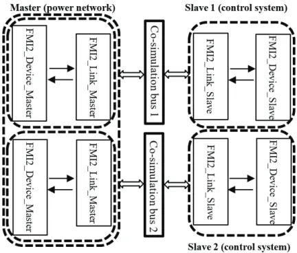
As previously mentioned, this new off-line simulation approach also adopts a master-slave co-simulation scheme. The control systems (slaves) are decoupled from the power network and encapsulated into FMUs which contain model and simulator information. The power network (master) then loads these FMUs without prior knowledge of their contents. As the simulation proceeds, the master communicates with the slaves through two layers of DLL files incorporating standardized FMI functions via a co-simulation bus composed of a shared memory zone (buffer) for data exchange, as well as associated synchronization mechanisms created by the master. This concept is illustrated in Figure 2.3 in which only two slave subsystems are shown for simplicity.

(40)

Figure 2.3 Interfacing three subnetworks (Master, Slave 1 and Slave 2) via DLL files and two co-simulation buses

FMI2_Device_Master defines the functions to interact with the EMTP solver, compatible with the FMI standard 2.0 functions defined and implemented in FMI2_Link_Master. FMI2_Device_Slave is in charge of interaction between a slave instance and EMTP, and FMI2_Link_Slave provides auxiliary coordination of master-slave data exchange by communicating with functions defined in FMI2_Link_Master. The contents of the latter two files are not constrained by the FMI standard. It is noted that a co-simulation bus is created for each slave instance in the simulation, and although a sperate set of master DLL files are used for every master-slave interface, they interact with the same solver instance in the master.

In the following sections, the definition, functionality and implementation of principal functions (whether defined in the FMI standard or designed for the interaction with the EMTP solver) in the 4 DLL files, as shown in Figure 2.3, are explained. Due to the high level of complexity in most of the implementation, the purpose and functionality of each function are summarized and made concise, and their implementation is explained in a descriptive manner. Detailed implementation of functions fmi2DoStep and stepFunc which are used to coordinate co-simulation between master and slaves is given in Appendix B for further references. Information with regards to the FMI function arguments and data types can be found in [19].

(41)

2.1.3.1 Implementation of functions in FMI2_Link_Master •_{fmi2Instantiate}

This function is called by the master program in order to load an FMU at the beginning of the co-simulation stage. It is called once for every slave (FMU) instance and returns an element of type “fmiComponent”. Its principal execution routines are:

1) Allocate memory for an FMU object 2) Assign certain values to the object

3) Create a file with a specified instance name in the same path where the FMU is extracted 4) Read values from the xml file and assign those values to the created FMU object

5) Read the location of the netlist file of the FMU • fmi2FreeInstance

This function releases the slave instance, that is to say, it releases all the memory allocated for the FMU.

• fmi2SetDebugLogging

This function allows the master to choose whether the FMU can send log messages to the master as well as the level of details in these messages.

•_{fmi2SetupExperiment}

This function asks the FMU to configure the co-simulation. It includes function calls to setINI and setIN [19].

• fmi2EnterInitializationMode

This function asks the FMU to enter the initialization mode in which variables with attributes “initial” = “exact” or “approx” can be defined. It is noted that the co-simulation bus used for data exchange between master and slave is realized by file mapping. Its main execution routines are:

1) Create the co-simulation bus, which is a file mapping object with a certain size 2) Create a map view associated with the file mapping object

(42)

3) Initialize certain elements in the co-simulation bus

4) Initialize all three synchronization semaphores by setting them to 0

5) Release semaphore SemInitialization to the slave, informing the slave that the co-simulation bus is successfully created and asking the slave to connect to it

• fmi2ExitInitializationMode

This function asks the FMU to exist the initialization mode. It executes the following routines: 1) Wait for the slave to release semaphore SemMaster to finish the initialization mode 2) Release SemMaster to itself so that the master can start its execution in the case of

asynchronous mode

Details on synchronization semaphores and different co-simulation modes will be explained hereinafter.

•_{fmi2Terminate}

This function notifies the FMU that the simulation is terminated by releasing the semaphore SemSlave one last time.

• fmi2Reset

This function demands that the FMU return to its initial state.

• fmi2SetReal, fmi2SetInteger, fmi2SetBoolean, fmi2SetString, fmi2GetReal, fmi2GetInteger, fmi2GetBoolean, fmi2GetString

These functions allow to transfer values from the master to the slave and vice versa. They are called at every simulation time-step of the master and can also be used to initialize variables in the FMU.

•_{fmi2GetStatus, fmi2GetRealStatus, fmi2GetIntegerStatus, fmi2GetBooleanStatus,} fmi2GetStringStatus

These functions are called by the master to require the status of the co-simulation. • fmi2DoStep

(43)

A call to this function starts the calculation of a new time-step in the FMU. It consists principally of the following execution routines:

1) Write the current communication point and the master numerical integration time-step onto the co-simulation bus

2) Read from the co-simulation bus the current slave time-point and its numerical integration time-step

3) Verify the co-simulation mode (synchronous or asynchronous) a) If the co-simulation mode is synchronous

i. If the slave lags behind the master

ii. Release semaphore SemSlave to the slave iii. Wait for semaphore SemMaster from the slave iv. Go back to i.

b) If the co-simulation mode is asynchronous

i. If the current communication time-point is 0 A. Release SemSlave to the slave

ii. If the current communication time-point is larger than 0 A. Wait for SemMaster from the slave

B. Release SemSlave to the slave 2.1.3.2 Implementation of functions in FMI2_Device_Master

Functions defined and implemented in this file are used for interaction between the FMI and EMTP solver. They are not constrained by the FMI standard and are executed by the master program.

• init

This function performs all necessary procedures in the initialization stage of the simulation. Its principal execution routines are: