Measuring and Analysing the Variations of Program Execution Times on Multicore Platforms: Case Study

(1)

HAL Id: inria-00514548

https://hal.inria.fr/inria-00514548v2

Submitted on 28 Sep 2010

HAL is a multi-disciplinary open access

archive for the deposit and dissemination of

sci-entific research documents, whether they are

pub-lished or not. The documents may come from

teaching and research institutions in France or

abroad, or from public or private research centers.

L’archive ouverte pluridisciplinaire HAL, est

destinée au dépôt et à la diffusion de documents

scientifiques de niveau recherche, publiés ou non,

émanant des établissements d’enseignement et de

recherche français ou étrangers, des laboratoires

publics ou privés.

Execution Times on Multicore Platforms: Case Study

Abdelhafid Mazouz, Sid Touati, Denis Barthou

To cite this version:

Abdelhafid Mazouz, Sid Touati, Denis Barthou. Measuring and Analysing the Variations of

Pro-gram Execution Times on Multicore Platforms: Case Study. [Research Report] 2010, pp.36.

�inria-00514548v2�

(2)

a p p o r t

ia-00514548--FR+ENG

Domaine 1

Measuring and Analysing the Variations of Program

Execution Times on Multicore Platforms: Case Study

Abdelhafid M

AZOUZ

— Sid-Ahmed-Ali T

OUATI

— Denis B

ARTHOU

N° HAL-inria-00514548

(3)

(4)

UFR des sciences 45 avenue des Etats Unis,

78035 Versailles cedex

Measuring and Analysing the Variations of Program Execution

Times on Multicore Platforms: Case Study

Abdelhafid Mazouz

∗

, Sid-Ahmed-Ali Touati

†

, Denis Barthou

‡

Domaine : Sciences et techniques ´

Equipe-Projet ARPA

Rapport de recherche n° HAL-inria-00514548 — July 2010 — 36 pages

Abstract: The recent growth in the number of precessing units in today’s multicore processor archi-tectures enables multiple threads to execute simultanesiouly achieving better performances by exploiting thread level parallelism. With the architectural complexity of these new state of the art designs, comes a need to better understand the interactions between the operating system layers, the applications and the underlying hardware platforms. The ability to characterise and to quantify those interactions can be useful in the processes of performance evaluation and analysis, compiler optimisations and operating system job scheduling allowing to achieve better performance stability, reproducibility and predictability. We consider in our study performances instability as variations in program execution times. While these variations are statistically insignificant for large sequential applications, we observe that parallel native OpenMP programs have less performance stability. Understanding the performance instability in current multicore architectures is even more complicated by the variety of factors and sources influencing the applications performances.

Key-words: OpenMP, Multicore, Parallelism, Performance evaluation

∗_{PRiSM, UVSQ. [email protected]} †_{PRiSM, UVSQ. [email protected]}

(5)

programmes sur un cas d’architecture multi-cœurs

Résumé : L’accroissement des unités de calculs dans les nouvelles architectures des processeurs multicœurs permet à plusieurs processus de s’exécuter simultanément afin d’obtenir des meilleures per-formances en exploitant un parallélisme de tâches. Avec la croissante complexité de ce nouveau type d’architectures, il est primordial de bien comprendre les interactions qui existent entre les couches du système d’exploitation, les applications et l’architecture matérielle. L’habilité de bien caractériser et de quantifier ces interactions peut être utile dans les processus d’évaluation et d’analyse des performances, des optimisations de code appliquées par le compilateur et pour l’ordonnanceur de tâches du système d’exploitation. Une bonne compréhension de ces intéractions peut conduire à une meilleure stabilité, reproductibilité et prédictibilité des performances.

Nous considérons dans notre étude que l’instabilité des performances est la variabilité dans les temps d’exécution des programmes. Bien que ces variations sont insignifiantes pour les applications séquentielles, nous avons observé que les programmes parallèles écrits avec le standard OpenMP ont moins de stabilité dans les performances. Comprendre cette instabilité dans le cadre des architectures multicœurs est rendu encore plus compliqué par la variété des facteurs et des sources influen¸cant les performances des applications.

(6)

1 Introduction

Multi-core architectures are nowadays the state of the art in the industry of processor design for desktop and high performance computing. With this design, multiple threads can run simultaneously exploiting a thread level parallelism. Unforunately, achieving better performances is a little bit hard work. Indeed, programmers have to deal with some issues in both software and hardware levels (thread and process scheduling, memory management, shared resources managements, energy consumption and heat dissi-pation of cores, etc.). Furthermore, the lack in understanding the interactions between the operating system layers, applications and the underlying hardware makes this task even more difficult. A good un-derstanding of these interactions may be exploited in performance evaluation, compiler optimisations and in process/thread scheduling to achieve a better performance stability, reproducibility and predictability. In this context, applications designers and performance analysts have to iteratively investigate how to achieve the best performances and checking the behaviour of their applications on that architectures. Most often, they consider the execution time as the first metric to investigate in the process of per-formance evaluation. The execution time is usually observed by measurements, or can be simulated or predicted with a performance model. In our study we consider direct measurements (either by hardware performance counters, or by OS timing functions calls). Contrary to emulated or virtualised programs (such as Javabyte-codes), native program binaries are executed directly on the hardware with possibly some basic OS requests (OS function calls). Our current study focuses on this family of programs: we consider the sample of SPEC 2006 and SPEC OMP2001 [1] benchmark applications. We do not consider binary virtualisation or byte-code emulation because they add software layers influencing the program performance in a more complex way: garbage collector strategies, threads organisation, caching and dynamic compilation techniques all may dramatically influence the measurements of program execution times. Direct measurements of native applications have one software layer (namely the OS) between the user code and the hardware. Unfortunately, the measurement process may also introduce errors or noise (the act of measuring perturbs the program being measured) that can affect our experimental results. For example, there is a time required to read a timer before the code to measure and store the timer after this code. Experimental setups may also introduce other factors that can lead to variation in program execution times. Some of these factors are: Interrupts, starting heap address, starting execution stack address, thread affinity, OS process scheduling policy, background process/thread, sharing of the last level of cache and environment size (that have been investigated in [2]). Thus, if we execute a program N times, we may obtain N distinct execution times.

In this document, we introduce some experiments aimed to measure, quantify and analyse the vari-ations of program execution times on an Intel multicore machine. We report measurement results for single-threaded applications (SPEC CPU2006), as well for parallel multi-threaded applications (SPEC OMP2001). The parallel applications use the OpenMP paradigm, one of the most used in parallel programming model on shared memory computers. We show in this study that large SPEC CPU2006 applications have minor variations with the train data input. This of course does not guarantee that the variations of sequential applications would always be negligible especially for small codes (kernels). Unlike single-threaded applications, we show that the variations of execution times of OpenMP applica-tions are really sensitive from a human user point of view.

The report is organised as follows. Section 2 introduces the experimental setup and methodology that we follow. Section 3 studies the performance variability of sequential applications (SPEC CPU 2006). The same study is conducted for parallel OpenMP applications in Sections 4 and 5. The influence of background co-running processes on the performances of OpenMP applications is studied in Section 6. Finally, Section 7 cites some related work before concluding.

(8)

Parameter Value

Linux Kernel X86 64 2.6.26

Linux patch perfmon kernel 2.81

Compilers gcc 4.1.3, gcc 4-3.2, icc 11.0, ifort 11.1

Benchmarks SPEC CPU2006, SPEC OMP2001, micro-benchmarks

Data input train

Micro-architecture Intel Core2

CPU Frequency 2.33 GHz

CPU number 2

Core number 8 (2 x 4)

System Memory 4G

Cache L1 32KB Ins, 32KB Data per 1 core

Cache L2 4MB per 2 cores

Table 1: Experimental Setup

2 Experimentation

2.1 Experimental setup

We use an Intel (Dell) server with two Clovertown processors. Each processor has 4 cores, while each couple of cores have a shared level 2 cache. Our system has two L2 caches on each chip with 4 MB, for both instructions and data. The core frequency is 2.33 GHz. The maim memory size is 4 GB RAM. The frontside bus has a clock rate of 1.33 GHz. The main features of the test machine are summarised in Table 1 and Figure 1.

4-MB L2 cache Core 0 Core 4 L1 cache 32KB D+32KB I 4-GB System Memory 1.33 GHz SYSTEM BUS 64 bits wide L1 cache 32KB D+32KB I 4-MB L2 cache Core 2 Core 6 L1 cache 32KB D+32KB I L1 cache 32KB D+32KB I 4-MB L2 cache Core 1 Core 5 L1 cache 32KB D+32KB I L1 cache 32KB D+32KB I 4-MB L2 cache Core 3 Core 7 L1 cache 32KB D+32KB I L1 cache 32KB D+32KB I

Intel 2.33 GHz Multicore Processor Core2 Micro-architecture Figure 1: Dual processor architecture

2.2 Experimental methodology

In order to improve the reproducibility of the results, the experiments were done following some practices: • The test machine was entirely dedicated during the experiments to a single user.

• Running each benchmarks 31 times [3,4] for each software configuration. This high number of runs allows us to report statistics with a high confidence level;1

• Unset all the shell environment variables that were inessential;

• The experiments were done on a minimally-loaded machine (disable all inessential OS services except sshd);

1_{We showed in [5] that the observed execution times of most of the applications do not follow a Gaussian distribution.}

This means that some statistical tests, such as the Studen t-test, cannot be conducted unless the sample size is large enough. It is commonly admitted that conducting more than 30 observations constitutes large samples [3, 4].

(9)

• Deactivation of the randomisation of the starting address of the stack (this is an option in the Linux kernel versions since 2.6.12);

• Dynamic voltage scaling (DVS) disabled;

• Using the build system and scripts of SPEC CPU2006 and OMP2001 to compile and optimise the applications, launch them, measure execution times, check validity of the results and report the performance numbers;

• The SPEC system measurement of execution times relies on the gettimeofday function; • The successive executions are performed sequentially in back-to-back way;

• No more than one application was executed at a time, except when we study co-running effects. • We use violin plot to report the program execution times of the 31 execution of each software

configuration. The Violin plot is similar to box plots, except that they also show the probability density of the data at different values. The white dot in each violin gives the median and the thick line through the white dot gives the inter-quartile range.

2.3 Definition of program performance variability

When we observe a sample of execution times of an application P , say {t1, · · · , tn} where ti is the

execution time of the ith_{run, then we may define the variability according to many metrics. Any used}

metric must define the feeling of the end user about the instability of the execution time of the application. We can use the usual sample variance, or | maxiti−miniti|

¯

t where ¯t is the sample mean, or

| maxiti−miniti| med(t)

where med(t) is the sample median. In our study, we use metrics that measure the disparity between extrema observations (outliers):

1. An absolute variability, which is the difference between the maximal and the minimal observed execution times AV (P ) = | maxiti− miniti|;

2. A relative variability, which is the absolute variability divided by the maximal observed execution time RV (P ) = AV (P )_max

iti =

| maxiti−miniti| maxiti .

Now the question is how to decide about a definition of a program with non negligible performance variability. Since any experimental measure brings a sample variation (it is impossible in practice to ob-serve exactly equal execution times), when can we speak about non negligible variability ? In our study, we say that a program P has non negligible performance variability if its absolute variability exceeds one second (AV (P ) > 1s) of if its relative variability exceeds 1% (RV (P ) > 1%). Another definition may exist; In our context we chose the previous definition in order to be close to the feeling of a user executing a program interactively (i.e. when he launches the program and he waits for its termination). The next section shows that the execution times of long running sequential applications have marginal variability.

3 Variability of SPEC CPU2006 execution times

This section presents the experiments related to the variability of SPEC CPU2006 program execution times. The considered source of variability is the UNIX shell environment size, as studied in [2].

The compiler used is gcc 4.1.3 with the flags -O2 and -O3. The option --fno-strict-aliasing was used for perlbench benchmark because of a technical error in that code2.

The experimentations done on SPEC CPU2006 benchmarks test the relation between the UNIX shell environment size and the variation of programs execution times. Following the methodology explained

2_{The benchmark has some known aliasing issues. Hence the compilation with high optimisation level will most likely}

produce binaries assuming strict aliasing. The problem was reported in the SPEC CPU2006 documentation.

(10)

in [2], we conducted our measurements by varying the size of the Unix shell environment (from 0 to 4095 bytes) and running each benchmark of SPEC CPU2006 31 times with the -O3 flag optimisation enabled of the gcc compiler and 31 times with the -O2 compiler flag.

Figure 2 shows the execution times of four applications under each Unix shell environment size using violin plot. The leftmost point of the X-axis is for a Unix shell environment size of 0 bytes (the null environment); we generated the data using the bash shell and for each point we added 63 bytes to the environment. The width of a violin plot at y-value y is proportional to the number of times we observed y. Figure 2 says that for each UNIX shell environment size in the X-axis, the Y-axis report the 31 execution times.

From all these figures we can deduce that: 1) the size of the Unix shell environment may influence the execution times and 2) the variations of execution times are minor and negligible (less than 1%). These observations are valid for all the SPEC CPU2006 benchmarks that we experimented.

Figure 3 reports the confidence interval of the mean of these benchmarks. We can see that these intervals are sufficiently tights. These figures shows that the sample mean at each Unix shell environment size does not vary in a significant way.

From the experiments presented in this section we deduce that varying the Unix shell environment size has a less impact (less than one second) on the variability of the execution times of SPEC CPU2006 benchmarks whatever the optimisation flag used (-O2 or -O3).

The next section shows the performance variability of the multi-threaded SPEC OMP2001 bench-marks given a fixed experimental setup.

4 Variability of SPEC OMP2001 execution times

This section presents experiments related to the variability of program execution times in SPEC OMP2001. The targeted benchmarks are parallel programs written with the OpenMP API. The aim of these exper-iments is to study two things: 1) Are the parallel execution of the benchmarks with different number of threads lead to variability in program execution times ? 2) Compare the benefit of the parallel execution with different number of threads against the sequential version.

The compilers used are gcc 4.3.2 and icc 11.0. For each application of SPEC OMP2001 bench-marks, we generated two compiled binary codes. The first one is generated by setting only the -O3 compilation flag (single-threaded version). The second one (multi-threaded version), is generated by setting -O3 -fopenmp and -O3 -openmp compilation flags respectively for the gcc and icc compilers. gcc was not able to compile the OpenMP version of mgrid m because of a bug (Bugzilla Bug 33904). The parallel execution of gafort m failed because of a segmentation fault (this execution error was also reported if we use the Intel icc compiler). The Unix shell environment size was fixed for each software configuration. In the case of the multi-threaded version, we consider 5 configurations. Each configura-tion sets up the number of thread to be generated at runtime. Typically, this is achieved by setting the environment variable OMP NUM THREADS respectively to the values 1, 2, 4, 6 and 8 threads. We limited OMP NUM THREADS to 8, because our experimental machine have a maximum number of cores equal to 8. Running a parallel version of each benchmark with only one thread may be surprising, but the goal of such approach is to compare the performances of the two configurations; (sequential code with -O3 and parallel code running with a single thread).

Figure 4 shows the violin plots of program execution times for four applications from SPEC OMP2001 benchmarks compiled using the gcc compiler. These applications are selected because they highlight significant performance variability. The X-axis represents the different software configurations for the application: sequential version (no threads), OMP version with 1 thread, 2 threads, 4 and 8 threads. The Y-axis represents the 31 observed execution times for each software configuration. We conclude the following observations:

(11)

59.2 59.6 60.0 0 441 945 1512 2142 2772 3402 4032 ●● ● ● ● ●●●● ● ● ● ●● ●●●● ●●●● ● ● ●●●●●_●●● ●● ● ● ● ● ● ● ●●● ●●●●●_●● ● ● ●● ●●●● ● ● ●●_●●● 401.bzip2 gcc −O3

bytes added to empty environment

Time(seconds) 1.41 1.43 1.45 0 441 945 1512 2142 2772 3402 4032 ●●●●●●●●● ● ●●●●●●●●●●●● ●●_●● ●●●●●●●●●●●●●●●● ● ●●●● ●●●● ● ●●● ●●●_●●● ●●●● 403.gcc gcc −O3

Time(seconds) 100.95 101.10 101.25 0 441 945 1512 2142 2772 3402 4032 ● ●● ●●● ●●● ● ●●● ●● ● ●●●●●●●●●●●●●●● ●●_● ● ●● ● ● ● ● ●●● ●●● ● ● ● ●●● ●● ●●● ●● ● ●●● ● 456.hmmer gcc −O3

Time(seconds) 29.0 29.5 30.0 30.5 0 441 945 1512 2142 2772 3402 4032 ● ● ● ●● ●●● ● ● ●●●● ●● ● ● ●●_● ● ●● ●●● ● ●_● ●● ●● ● ● ●●●●●●●●●● ● ● ● ●● ●_● ●● ● ●●● ● ●●● ●● 429.mcf gcc −O3

Time(seconds)

Figure 2: Observed Execution Times of some SPEC CPU 2006 Applications (compiled with gcc)

●● ● ● ● ●●● ● ●● ● ● ● ● ●● ●● ●●● ● ● ● ● ● ● ● ● ● ● ●● ● ● ● ● ● ● ● ●● ●●●●● ●● ● ● ●● ●●● ● ● ● ● ● ● ● ● 0 756 1575 2394 3213 4032 59.3 59.5 59.7 401.bzip2 gcc −O3 Confidence level 95% bytes added to empty environment

Time(seconds) ●_● ● ● ●● ●● ● ● ● ● ●● ● ● ● ●● ● ● ● ●● ● ● ●●●● ● ●● ●●●● ● ● ● ● ● ● ● ●● ● ● ● ● ● ● ●● ● ● ● ● ● ● ● ● ● ● ● 0 756 1575 2394 3213 4032 1.418 1.422 1.426 403.gcc gcc −O3 Confidence level 95% bytes added to empty environment

Time(seconds) ● ●●● ●_● ●●● ● ●●●●● ● ●●●● ●●●●● ●●●●●● ●●_● ● ●● ● ● ● ● ●●● ●●● ● ● ● ●●● ●● ●●● ●● ● ●●● ● 0 756 1575 2394 3213 4032 100.95 101.10 101.25 456.hmmer gcc −O3 Confidence level 95% bytes added to empty environment

Time(seconds) ● ● ● ●● ●● ● ● ● ● ● ● ● ●● ● ● ●● ● ● ● ● ● ●● ● ● ● ● ● ● ● ● ● ● ●●● ●● ● ● ●● ● ● ● ●● ● ● ● ● ● ● ●_● ● ● ● ● ●● 0 756 1575 2394 3213 4032 29.2 29.6 30.0 429.mcf gcc −O3 Confidence level 95% bytes added to empty environment

Time(seconds)

Figure 3: Mean 95% Confidence Interval of some SPEC CPU 2006 Applications (compiled with gcc) UVSQ

(12)

1. The sequential and the single threaded versions do not exhibit significant variability.

2. When we use thread level parallelism (2 or more threads), the execution times decreases in overall but with a significant disparity. Consider for instance the case of swim in Figure 4. The version with 2 threads runs between 76 and 109 s, the version with 4 threads runs between 71 and 90 s. This variability is also present when swim is compiled with icc, see Figure 5. The example of wupwise in Fig. 4 is also interesting. The version with 2 threads runs between 376 and 408 s, the version with 6 threads runs between 187 and 204 s. This disparity between the distinct execution times of the same program with the same data input cannot be justified by accidents or experimental hazards. Applying the Shapiro-Wilk normality check on performance data we concluded that the execution times are not normally distributed, and frequently have a bias.

3. The case of the application galgel is also interesting. In addition to the variability of the execution times for each software configuration, we observe that the performance of the program substantially decreases when increasing the number of threads! This examples illustrates that, on a multicore architecture, increasing thread parallelism may bring severe performance loss. We checked the situation of galgel when we use the Intel icc 11.0 compiler instead of gcc, and the situation was radically different, see Figure 5: increasing the number of threads decreases the execution times. We can observe a huge difference between the performance of the program compiled with gcc vs. the icc, either in terms of execution times and in terms of variability. We have to notice that using the gcc-4.4.3 version of the GNU compiler has effectively reduced the execution times when we increase the number of threads (see Figure 6). This situation illustrate that the quality of the code generated by a compiler has a significant impact on performance stability.

4. The galgel application compiled with the gcc compiler, shows that speedup computation is not fair if we consider the minor execution time. We can see from the Figure 4 that the violin plots of the second (PAR (1TH)) and third (PAR(2TH)) configurations gives an interesting result on how we have to summarise the performance data of one configuration to single number. If we use the min function to summarise data of the two configurations, then, we can say that the third configuration is better than the second one. But if we take the median function to summarise these data we may conclude that the two configurations are similar. We note that the choice of which function to use to define the execution time is crucial and may lead to misleading conclusions about the real behaviour of the system.

5. Figure 7 shows that the sequential version of ammp is better than his parallel version when par-allelisation is achieved with: 1 thread by about 25%, and 2 threads by about 15%. The case of ammp shows that the OpenMP API does not necessarily produce faster codes against the sequential version. The reason is that the compiler makes better optimisations when OpenMP is not enabled. 6. When the number of threads is equal to 8, then the variability is significantly reduced on the 8

cores machine.

The next section presents a study of the effect of running real applications with an affinity to the system cores taking into account the impact of sharing the last level cache (L2 cache).

5 Study of the impact of thread affinity on SPEC OMP2001

execution times

In the previous section, we have seen the relation between performances variability and the effect of co-running independant background processes. We conduct the following experiments aiming to check the impact of changing the scheduling affinity of SPEC OMP2001 threads on performances variability (studied in Section 4). When affinity is enabled, we mean that we fix the placement of the threads on the cores of the processor.

We used the gcc 4.4.3 and icc 11.0 compilers. For each SPEC OMP2001 application, we generated a multi-threaded version of each benchmark by setting -O3 -fopenmp and -O3 -openmp compilation flags

(13)

70 80 90 100 110 120

SEQ PAR (1TH) PAR (2TH) PAR (4TH) PAR (6TH) PAR (8TH)

● ●

●

● ●

●

312.swim_m

gfortran−4.3.2: −O3 vs −O3 −fopenmp

Time(seconds) 200 300 400 500 600 700

● ● ● ● ● ● 310.wupwise_m

Time(seconds)

80

100

120

140

● ● ● ● ● ● 318.galgel_m

Time(seconds) 20 25 30 35 40 45 50 55

● ● ● ● ● ● 320.equake_m

gcc−4.3.2: −O3 vs −O3 −fopenmp

Time(seconds)

Figure 4: Observed Execution Times of some SPEC OMP 2001 Applications (compiled with gcc)

70 80 90 100 110 120

● ● ● ● ● ● 312.swim_m

ifort−11.1: −O3 vs −O3 −openmp

Time(seconds) 200 300 400 500 600 700

● ● ● ● ● ● 310.wupwise_m

Time(seconds)

30

40

50

60

● ● ● ● ● ● 318.galgel_m

Time(seconds) 15 20 25 30 35 40

● ● ● ● ● ● 320.equake_m

Time(seconds)

Figure 5: Observed Execution Times of some SPEC OMP 2001 Applications (compiled with icc)

(14)

30 40 50 60 70 80 90

SEQ PAR (1TH) PAR (2TH) PAR (4TH) PAR (6TH) PAR (8TH) ● ● ● ● ● ● 318.galgel_m

Time(seconds)

Figure 6: Observed Execution Times of the galgel benchmark compiled with gcc-4.4.3

100

120

140

160

180

● ● ● ● ● ● 332.ammp_m

gcc−4.3.2: −O3 vs −O3 −fopenmp

Time(seconds)

Figure 7: Observed Execution Times of ammp m benchmark (compiled with gcc)

100

150

200

● ● ● ● ● ● 332.ammp_m

icc−11.0: −O3 vs −O3 −openmp

Time(seconds)

Figure 8: Observed Execution Times of ammp m benchmark (compiled with icc)

respectively for the gcc and icc compilers. We run each application with respectively 2, 4 and 6 threads under three runtime configurations :

1. Running the benchmarks without scheduling affinity (affinity disabled, threads placement let to the OS).

2. Running the benchmarks under the icc compiler compact [6] affinity strategy. Specifying compact as affinity assigns the OpenMP thread n + 1 to a free core as close as possible to the core where the OpenMP thread n was placed3_{. We experiment this affinity strategy because it leads to increase}

the L2 cache sharing between threads, even if not all the applications can take advantage from it. 3. Running the benchmarks under the icc compiler scatter [6] strategy. Specifying scatter affinity strategy distributes the threads as evenly as possible across the entire system. Scatter is an opposite affinity strategy compared to compact. Running applications under this strategy may be benifical to alleviate the problem of system bus contention of neighbours cores.

Figure 13 and Figure 14 show violin plots of program execution times (CPU time) for the wupwise and swim applications (from SPEC OMP2001 benchmarks) compiled with the gcc and icc compilers. In each figure, three violin plots report the execution times when the benchmarks are launched with

3_{For example, in a topology map, the nearer a node (group of processors) to the root, the more significance the node}

(15)

40

60

80

100

120

● ● ● ● ● ● 316.applu_m

Time(seconds) 4.4 4.6 4.8 5.0 5.2 5.4 5.6

● ●

●

● ●

330.art_m

Time(seconds) 80 100 120 140 160 180 200

● ● ● ● ● ● 328.fma3d_m

Time(seconds) 60 80 100 120 140 160

● ●

●

● ●

324.apsi_m

Time(seconds)

Figure 9: Observed Execution Times of some SPEC OMP2001 Applications (compiled with gcc)

20 40 60 80 100 120

● ● ● ● ● ● 316.applu_m

Time(seconds) 4.6 4.8 5.0 5.2 5.4 5.6 5.8 6.0

● ● ● ● ● ● 330.art_m

Time(seconds)

60

80

100

120

● ● ● ● ● ● 328.fma3d_m

Time(seconds) 40 60 80 100 120 140 160

● ● ● ● ● ● 324.apsi_m

Time(seconds)

Figure 10: Observed Execution Times of some SPEC OMP2001 Applications (compiled with icc)

(16)

2, 4 and 6 threads. The X-axis represents the three affinity configurations (no fixed affinity, compact, scatter). The Y-axis represents the 31 observed execution times for each configuration. We make the following observations:

1. When the scheduling affinity is disabled, we observe a significant variability in execution times for SPEC OMP2001 benchmarks. If we consider the case of swim in Figure 14 compiled with gcc, the version with 2 threads runs between 79 and 110 s, the version with 4 threads runs between 73 and 90 s and the version with 6 threads runs between 71 and 82 s. Figure 14 shows that when the benchmark is compiled with the icc compiler, it exhibits a variability too.

2. The variability is insignificant in almost all the benchmarks when the schedlung affinity is enabled (the observed variability is less than 1.5%). The variability disappears either when the threads shares L2 cache (compact binding) or not (scatter binding). Figure 13 shows for the wupwise application compiled with gcc that the version with 2 threads runs ≈ 454 s when they shares the L2 cache (2 threads runs on 2 cores sharing single L2 cache compact) and runs between 419 and 421 s when they do not share it scatter.

3. The art benchmark used with both compilers and the apsi with gcc exhibits a less sensitivity to changing scheduling affinity. We observed that even when we set up the binding feature, variability in execution times still appear (see Figures 15 and 16 where the variability exceeds 5%). In other words, fixing the affinity between the threads does not remove the performance variability of all the benchmarks.

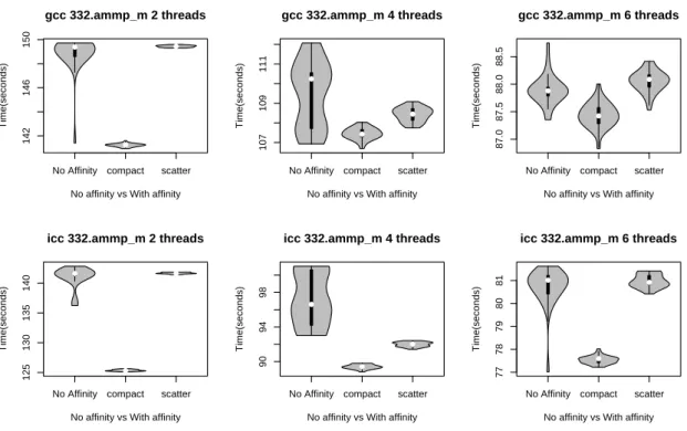
4. We observed in 7 from the 9 tested benchmarks that they run faster when they are launched with a scatter strategy). The benchmarks which take benefits from L2 cache sharing compact are ammp and galgel with both compilers (see Figures 17 and 18).

In order to check the origin of the performance variability observed when we disable the affinity, we study the impact of thread placements (fixed by the OS) on the cache effects. For instance, we run swim and we report his number of last level cache misses (L2 cache misses). Figure 12 shows violin plots summarising the number of L2 cache misses when swim runs with 2 threads. We observe clearly that the variability of the execution times observed in Figure 11 is closely related to the number of L2 cache misses. Indeed, when we binded the threads of swim explicitly to the system cores, we observed insignif-icant variability in the execution times. But whacking system to handle the threads placement on the cores the situation was completely different and we observed an important variability. The interesting thing is that higher execution time in the configuration without affinity was accompanied with a higher L2 cache misses number. This situation shows that swim is sensitive to cache affinity.

When affinity is not fixed, the increase of the number of L2 cache misses does not explain the cause of the observed performance variability but just an effect. We observe that the an important factor contributing to the important performance variability is the thread migration operated by OS kernel. Indeed, we traced the mapping of threads to cores each time a new parallel region is entered. The analysis of the tracing of the mapping event allows us to see that the runs with high execution times, the application threads have suffered from a thread migration. Thus, the migration impact negatively the cache utilisation leading to a significant performance variability. However, it is possible that thread migration improves execution times: this is the case for instance when date reuse and L2 cache sharing less important.

In addition to swim, we observed also that the performances of wupwise, applu, equake, apsi, fma3d, ammp applications are sensitive to cache affinity too.

In this section, we clearly observe that fixing affinity between threads removes performances variability in many applications, but not all: there are still other influencing factors that make executions time to vary. By now, it is not clear if fixing affinity would improve the average or the median execution time. Sometimes, it is better to let some hazard (OS) to decide about thread binding, since it is not clear if simple strategies such as scatter and compact are efficient.

(17)

80

90

100

110

No Affinity compact scatter

●

icc 312.swim_m 2 threads

No affinity vs With affinity

Time(seconds)

Figure 11: Observed cycles count in swim running with 2 threads

4e+08

6e+08

8e+08

1e+09

No bind compact scatter

●

icc 312.swim_m 2 threads

L2_LINES_IN:SELF

Figure 12: Observed L2 cache lines misses in swim running with 2 threads

420

430

440

450

No Affinity compact scatter ●

●

● gcc 310.wupwise_m 2 threads

Time(seconds)

250

260

270

280

●

Time(seconds)

195

200

205

●

Time(seconds)

400

410

420

430

●

● icc 310.wupwise_m 2 threads

Time(seconds)

240

250

260

270

●

Time(seconds)

190

195

200

205

●

Time(seconds)

Figure 13: Observed Execution Times of the wupwise Application (compiled with gcc and icc)

(18)

80

90

100

110

●

● gcc 312.swim_m 2 threads

Time(seconds)

75

85

95

105

●

Time(seconds)

72

76

80

●

Time(seconds)

80

90

100

110

●

● icc 312.swim_m 2 threads

Time(seconds)

70

80

90

100

●

Time(seconds)

72

76

80

●

Time(seconds)

Figure 14: Observed Execution Times of the swim Application (compiled with gcc and icc)

4.8

5.0

5.2

5.4

●

● gcc 330.art_m 2 threads

Time(seconds)

4.5

4.7

4.9

● ● gcc 330.art_m 4 threads

Time(seconds)

4.5

4.7

4.9

● ●

● gcc 330.art_m 6 threads

Time(seconds) 5.0 5.2 5.4 5.6 5.8

●

● icc 330.art_m 2 threads

Time(seconds) 5.0 5.1 5.2 5.3 5.4

●

● icc 330.art_m 4 threads

Time(seconds)

4.8

5.0

5.2

5.4

● ● ●

icc 330.art_m 6 threads

Time(seconds)

(19)

93

94

95

96

97

●

● gcc 324.apsi_m 2 threads

Time(seconds)

56

58

60

62

●

Time(seconds) 52 53 54 55 56

● _●

Time(seconds) 82 83 84 85 86 87

●

● icc 324.apsi_m 2 threads

Time(seconds) 50 51 52 53 54 55

●

● icc 324.apsi_m 4 threads

Time(seconds)

44.0

45.0

46.0

● ● icc 324.apsi_m 6 threads

Time(seconds)

Figure 16: Observed Execution Times of the apsi Application (compiled with gcc and icc)

52

54

56

58

60

● ● gcc 318.galgel_m 2 threads

Time(seconds) 36 37 38 39 40 41

Time(seconds)

31.5

32.5

33.5

Time(seconds) 36 38 40 42 44

● ● icc 318.galgel_m 2 threads

Time(seconds) 28 29 30 31 32

Time(seconds)

25.5

26.5

27.5

Time(seconds)

Figure 17: Observed Execution Times of the galgel Application (compiled with gcc and icc)

(20)

142

146

150

● ● gcc 332.ammp_m 2 threads

Time(seconds)

107

109

111

Time(seconds)

87.0

87.5

88.0

88.5

Time(seconds)

125

130

135

140

● ● icc 332.ammp_m 2 threads

Time(seconds)

90

94

98

Time(seconds) 77 78 79 80 81

Time(seconds)

Figure 18: Observed Execution Times of the ammp Application (compiled with gcc and icc)

6 Study of co-running processes impact on programs

perfor-mance variability

This section describes experiments trying to quantify and qualify the factors influencing the variations of program execution times. One of the factors which can influence the variability of program execution times is the core resource sharing. In our study, we focus on the sharing between the OpenMP parallel programs and some artificial applications. For each OpenMP benchmark we retrieve its execution times in user mode (run level 3 : least privileged mode), system mode (run level 0 : most privileged mode) and real execution time (total elapsed execution time).

In these experiments we generate a system load by running some artificial co-running processes in background. These processes are launched by one process executing the fork system call a number of times equal to the number of processes that we need to generate at runtime. This number is supplied as an argument to the command line. The code executed by these co-running processes is a dummy non terminating loop without memory access. The code of the co-running processes is given by Listing 3 in page 21.

6.1 Experimental setup

• Each benchmark was compiled with the -O3 -fopenmp flags.

• The OpenMP program execution time measurement is only done on thread number 0 (we retrieve the execution time of the master thread because it is the one that defines the whole application execution time).

• The SPEC OMP2001 benchmarks are launched with 8 threads at runtime. • We have five runtime configurations:

(21)

• Each SPEC OMP2001 benchmark (8 threads) is run either as a single application on the machine (minimal system load) or in parallel with 8, 16, 24 or 32 co-running processes respectively (perfor-mance perturbation created in background). This leads to five distinct runtime configurations. • The SPEC OMP2001 and the co-running processes are launched without scheduling affinity to the

system cores (no explicit binding of threads on cores).

• The number of the OpenMP threads (from applications under study) and co-running processes running on each core are respectively : 1, 2, 3, 4 and 5. For example a configuration with 5 threads or co-running process per core, consist of 1 OpenMP thread plus 4 co-running processes.

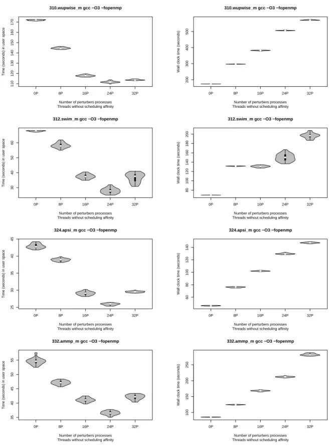
Figure 19 and Figure 20 show the violin plots of the user and real program execution times for four applications from SPEC OMP2001 benchmarks compiled using the gcc-4.3.2 compiler. The X-axis represents the violin plots of program execution times when the SPEC OMP2001 benchmarks run to-gether with the co-running processes. The Y-axis represents the 31 observed execution times for each software configuration.

From Figure 19, we can see that when we increase the number of processes running in background, the program execution times at user level of the OpenMP applications decreases. Meanwhile we observe in Figure 20 an increase of real execution times. Running the threads of the SPEC OMP2001 benchmarks and the co-running processes with a fixed scheduling affinity leads to the same conclusion (not plotted here): when we increase the number of co-running processes, we observe a decrease in program execution times at user level of the OpenMP applications. The following section presents measurements to check if the phenomenon presented above appears when running some basic micro-benchmarks instead of SPEC OMP2001.

6.2 Study of system load impact on micro-benchmarks execution times

We follow the same steps presented in the previous section, but this time we use some synthetic (simple codes) benchmarks which we call micro-benchmarks. These micro-benchmarks are used to isolate some micro-architectural events. All of the micro-benchmarks and the co-running processes were compiled with the compiler optimisation flag -O3.

6.2.1 Micro-benchmarks code

The code of the micro-benchmarks in Listing 1 (page 20) is composed of three loops Loop1 (paral-lel loop), Loop2, Loop3 and one statement S1. The L2 loop is added for repetition purpose to in-crease the measurement accuracy. The data set accessed by all the micro-benchmarks is equal to N ∗ M ∗ sizeof (int64) = D bytes where N is the number of iterations of the outermost loop (Loop1 loop) and M is the number of iterations of the inner most loop (Loop3 loop). In addition, since we want to give the same workload to every thread, this leads to consider values for N which are multiple of the number of threads. Having all this constraints, the values taken by N are from 8 to 196608 and the values taken by M are from 196608 to 8. For instance, when we have 8 threads, the value of N starts at 8. Furthermore, whatever the values of N and M are, the workload assigned to each thread has a working set of size 1.5M B. This size is chosen to be less than the half of the size of the L2 cache preventing from frequently accessing the DRAM in case of L2 cache misses.

Now we define the notion of memory chunk. In the context of our study the chunk represents the size of the vector fraction from tab accessed by the innermost M-loop: in the peticular code of Listing 1, we clearly see that each iteration of the M-loop accesses to a single element from tab, consequently chunk size = M × sizeof (int64). Table 2 gives the couples of values of N and M that we have experimented. To every couple of values (N,M) we associate the micro-benchmark mb N-value M-value. Following this denomination, the first micro-benchmark is mb 8 196608, the second mb 16 98304 and so on. With this micro-benchmark structure, we access the array tab in an indexed way represented by the S1 statement. Thus, the size of the chunk accessed in the M-loop depends on the number of iterations of the Loop1. So, Larger values of N lead to smaller sizes of chunks. In contrary, smaller values of N lead to larger sizes of chunks.

(22)

110 120 130 140 150 160 170 0P 8P 16P 24P 32P ● ● ● ● ●

310.wupwise_m gcc −O3 −fopenmp

Threads without scheduling affinity Number of perturbers processes

Time (seconds) in user space

30 40 50 60 0P 8P 16P 24P 32P ● ● ● ● ●

312.swim_m gcc −O3 −fopenmp

25 30 35 40 45 0P 8P 16P 24P 32P ● ● ● ● ●

324.apsi_m gcc −O3 −fopenmp

35 40 45 50 55 0P 8P 16P 24P 32P ● ● ● ● ●

332.ammp_m gcc −O3 −fopenmp

Figure 19: Observed User Execution Times of some SPEC OMP2001 Applications (compiled with gcc)

200 300 400 500 0P 8P 16P 24P 32P ● ● ● ● ●

310.wupwise_m gcc −O3 −fopenmp

Wall clock time (seconds)

80 100 120 140 160 180 200 0P 8P 16P 24P 32P ● ● ● ● ●

312.swim_m gcc −O3 −fopenmp

60 80 100 120 140 0P 8P 16P 24P 32P ● ● ● ● ●

324.apsi_m gcc −O3 −fopenmp

100 150 200 250 0P 8P 16P 24P 32P ● ● ● ● ●

332.ammp_m gcc −O3 −fopenmp

Figure 20: Observed Real Execution Times of some SPEC OMP2001 Applications (compiled with gcc)

(23)

N M Benchmark Chunk size = M*sizeof(int64)

N M Benchmark Chunk size =

M*sizeof(int64) 8 196608 mb 8 196608 1536 KB 1536 1024 mb 1536 1024 8 KB 16 98304 mb 16 98304 768 KB 3072 512 mb 3072 512 4 KB 32 49152 mb 32 49152 384 KB 6144 256 mb 6144 256 2 KB 64 24576 mb 64 24576 192 KB 12288 128 mb 12288 128 1 KB 128 12288 mb 128 12288 96 KB 24576 64 mb 24576 64 0.5 KB 256 6144 mb 256 6144 48 KB 49152 32 mb 49152 32 0.25 KB 512 3072 mb 512 3072 24 KB 98304 16 mb 98304 16 0.125 KB 1024 1536 mb 1024 1536 12 KB 196608 8 mb 196608 8 0.0625 KB

Table 2: Values taken by N and M in the outermost and the innermost loops of th micro-benchmarks code

Listing 1: OpenMP micro-benchmarks code void w a s t e t i m e ( ) {

#pragma omp p a r a l l e l f o r d e f a u l t ( none ) p r i v a t e ( i , j , k ) s h a r e d ( t a b ) Loop1 : f o r ( i = 0 ; i < N ; i ++)

Loop2 : f o r ( j = 0 ; j < 1 0 0 0 0 ; j ++)

Loop3 : f o r ( k = 0 ; k < M; k++)

S1 : ta b [ i∗M+k]++;

}

The first micro-benchmark mb 8 196608 corresponds to the case where every thread executes a single outer loop iteration (Loop1 or the N-loop) and the innermost loop M-loop accesses to a chunk of size M ∗ sizeof (int64) = 1.5 M B. This chuck size is sufficient to keep data inside the L2 cache but not inside the L1 data cache. In other words, the first micro-benchmark guarantees that every thread has its data in L2 but not in L1.

The last micro-benchmark mb 196608 8 corresponds to the case where every thread executes N/8 = 24576 N iterations, the innermost M-loops access to a chunk of size M ∗ sizeof (long) = 64 B (a single cache line size). In other words, this last micro-benchmark guarantees that every thread has all its data in L1.

The other micro-benchmarks between mb 8 196608 and mb 196608 8 cover the range for other values of (N,M). They give us the performance of the intermediate situations when data are fully or partly in L1. We should have (in theory) all data fully inside L2 because the chunk sizes are all less than half of L2 size, but we see later that threads sharing common L2 may create cache conflicts, thus data are ejected from L2.

Listing 2 shows the code of the co-running processes executing in parallel with Listing 1. We can see that it is a simple code consisting of a dummy non terminating while loop. The stress function is called by the main function and it never returns unless there is an explicit user intervention by sending the Linux SIGINT signal to stop it.

Listing 2: co-running processes code i n t s t r e s s ( ) { while ( 1 ) { ; } return 0 ; } UVSQ

(24)

The generated assembly code after compiling the C code of the co-running processes with the -O3 compilation flag is given in listing 3.

Listing 3: The

generated assembly code of the func-tion stress in the co-running process code

. l a b e l :

jmp . l a b e l

6.2.2 Micro-benchmarks execution times under co-running processes

In this section, the micro-benchmarks are run with 8 threads. The binding of the thread is fixed as follows: thread i is fixed to be executed on core i. Since the machine has 8 cores, each thread of the micro-benchmark is devoted to a single core. On that core, other co-running processes are launched with a fixed round-robin affinity: co-running process i is scheduled to be run on core number i modulo 8.

From Figure 21, we observe that when we increase the number of co-running processes per core (X-axis), a decrease holds for program execution times at user level. This observation is done with the mb 8 196608, mb 64 4576 and mb 256 6144 micro-benchmarks, but a slight increase of user level execution time is observed in the mb 512 3072 micro-benchmark. Furthermore, we observe that all the micro-benchmarks which have a N value in the outermost loop (the i loop) greater or equal than 512 (chunk sizes less than 32KB), have a slight increase (can be neglected) in program execution times at the user level. At the other side, all the micro-benchmarks which have a N value less than 512 (chunk sizes greater than 32 KB), have a noticeable decrease of program execution time at the user level.

The common point between the micro-benchmarks where the program execution times decrease is the size of the chunk that each thread treats. Indeed, each thread from those benchmarks treats a chuck which have a size greater than 32 KB. The size of those chunks fits in the L2 cache but it does not fit in L1 data cache leading to frequently access the last level cache. In addition, the benchmarks presenting a decrease in program execution times exhibits a high number of L2 cache misses. This phenomenon does not appear in the mb 512 3072 benchmark. For each iteration of the i loop in this micro-benchmark, a 24KB data size are provided to the L1 data cache which have a 32KB size.

Another remark is that the mb 512 3072 micro-benchmark has the least program execution time com-pared to the other micro-benchmarks. Even if there are some micro-benchmarks which have program execution times decrease, mb 512 3072 still have the minimal observed execution time.

Now let try to understand the performances of Figure 21 by plotting the L2 cache miss rate in Figure 22:

1. We have 8 threads running on eight 8 and 4 L2 caches, each L2 cache is shared between two cores (see the architecture of the machine in Figure 1 in page 5). Then we have two threads running on two adjacent cores meaning that they are competing to access a shared L2 cache. The decrease of execution times was observed on micro-benchmarks which access chunks having a size greater than the size of the L1 data cache. Thus, this subset of micro-benchmarks needs a high frequency access of the L2 cache to provide the needed data by the L1 data cache leading to a high number of L1 data cache misses.

2. The high number of L2 cache misses observed can be due to the hardware prefetcher of the L2 cache. We think that the automatic hardware prefetcher evict some useful data from L2. The main effect of prior behaviour, is for each iteration of Loop2 (the j loop), data must be reloaded to the L2 cache leading to the high number of L2 cache misses. Another explanation for the high number

(25)

1.5 2.0 2.5 3.0 0P 1P 2P 3P 4P ● ● ● ● ● gcc mb_8_196608 −O3 −fopenmp

Number of processes added per core

Cycles count in user space (seconds)

1.27254 1.27260 1.27266 0P 1P 2P 3P 4P ● ● ● ● ● gcc mb_512_3072 −O3 −fopenmp

Figure 21: Observed User Execution Times of some micro-benchmarks (compiled with gcc)

0e+00 2e+06 4e+06 0P 1P 2P 3P 4P ● ● ● ● _● gcc mb_8_196608 −O3 −fopenmp

Cache L2 misses in user space

1000 1500 2000 2500 0P 1P 2P 3P 4P ● ● ● ● ● gcc mb_64_24576 −O3 −fopenmp

Figure 22: Observed L2 cache misses of some micro-benchmarks (compiled with gcc)

(26)

of L2 cache misses is due to using small virtual memory pages. In this case several 4 KB pages are mapped to the block of L2 cache lines, resulting in conflict misses.

From the foregoing facts, we emit another hypothesis trying to explain why user-level program exe-cution times decrease when we increase the number some co-running processes. The hypothesis is based on the influence of the thread scheduling policy (Round-Robin time sharing) on the execution times. We think that the threads running on cores sharing data in L2 will not access them simultaneously: for each couple of cores sharing an L2 cache, the scheduling of the thread may lead to situations where one core will run an OpenMP thread and the adjacent core will run the co-running process resulting in none simultaneously access to the shared L2.

Therefore, the number of L2 cache misses decreases, reducing the pressure on the shared L2 cache. Finally, this situation leads to decrease the program execution times at the user level. The following subsection presents experiments to check the relevance of our hypothesis.

6.2.3 The impact of thread affinity on micro-benchmarks execution times

The aim of these experiments is to study the role played by the co-running processes on the decrease of program execution times at user level. To achieve this goal, we conducted our experiments following the experimental setup presented in Section 6.1 with some modifications at the runtime level.

• The micro-benchmarks are launched with 4 threads at runtime.

• Each micro-benchmark (4 threads) is run either alone as a single application on the machine (minimal system load) or in parallel with with 4, 8, 12 or 16 co-running processes (so we experiment five runtime configurations).

• We have also two scheduling affinity configurations:

1. The micro-benchmarks threads and the co-running processes are launched on the system cores 0, 1, 4 and 5, where cores 0 and 4 share one L2 cache, similarly cores 1 and 5 share another L2 cache (see Figure. 1 in page 5).

2. The micro-benchmarks threads and the co-running processes are launched on the system cores 0, 1, 2 and 3, where there is no sharing of L2 cache between these cores.

• The number of co-running processes running on each core varies from 0 to 4. If we add the thread of the micro-benchmark, then the number of running threads and processes on every core varies between 1 and 5. Since we use only 4 cores within 8 (see above), it means that the overall number of co-running processes on the system vary from 0 to 16. On every core, the co-running processes are launched with a fixed round-robin affinity on the experimented cores.

The main difference of this experiment against the last one presented in Section 6.2.2, appears in the way the threads of the benchmarks run. You should notice that in this experiment, the number of threads of the micro-benchmarks used at runtime is four. These threads are launched with a scheduling affinity to cores in two manners: 1) configuration where there are share of the L2 cache between the threads, and 2) configuration where there are no L2 cache sharing. To allow a comparison between the actual experiment and the last one (Section 6.2.2), threads must treat the same data size. To achieve this goal, we changed the N and M values of Listing 1 to run the micro-benchmarks with four threads. Thus, we keep the same data size accessed by each thread as in the case where micro-benchmarks were launched with eight threads. The new values taken by N are from 4 to 196608 and from 196608 to 4 for the M parameter in the micro-benchmarks code.

Figure 23 and Figure 25 illustrate the results when the micro-benchmarks threads and the co-running processes are binded to system cores 0, 1, 4 and 5 and to system cores 0, 1, 2 and 3 respectively. From Figure 23 we can see that program execution times at user level still decrease in the mb 4 196608, mb 16 24576 and mb 128 x6144 micro-benchmarks. We can also observe in Figure 23 that the execution times of mb 256 3072 increase. We clearly observed the phenomena of program execution times decreas-ing when 1) each couple of the micro-benchmarks threads share an L2 cache and 2) the sum of the array

(27)

1.5 2.0 2.5 0P 1P 2P 3P 4P ● ● ● _● ● gcc mb_4_196608 −O3 −fopenmp Perturb Cores 0 1 4 5 Number of Processes added per core

1.35 1.45 1.55 1.65 0P 1P 2P 3P 4P ● ● ● ● ● gcc mb_16_49152 −O3 −fopenmp Perturb Cores 0 1 4 5 Number of Processes added per core

1.35 1.45 1.55 1.65 0P 1P 2P 3P 4P ● ● ● ● ● gcc mb_128_6144 −O3 −fopenmp Perturb Cores 0 1 4 5 Number of Processes added per core

1.27306 1.27312 0P 1P 2P 3P 4P ● ● ● ● ● gcc mb_256_3072 −O3 −fopenmp Perturb Cores 0 1 4 5 Number of Processes added per core

Figure 23: Observed User Execution Times of some micro-benchmarks binded to the 0, 1, 4 and 5 cores

0e+00 2e+06 4e+06 0P 1P 2P 3P 4P ● ● ● ● ● gcc mb_4_196608 −O3 −fopenmp Perturb Cores 0 1 4 5 Number of Processes added per core

1000 1500 2000 2500 0P 1P 2P 3P 4P ● ● ● ● ● gcc mb_16_49152 −O3 −fopenmp Perturb Cores 0 1 4 5 Number of Processes added per core

1000 1500 2000 0P 1P 2P 3P 4P ● ● ● ● ● gcc mb_128_6144 −O3 −fopenmp Perturb Cores 0 1 4 5 Number of Processes added per core

Figure 24: Observed L2 cache misses of some micro-benchmarks binded to the 0, 1, 4 and 5 cores

(28)

1.372 1.376 0P 1P 2P 3P 4P ● ● ● ● ● gcc mb_4_196608 −O3 −fopenmp Perturb Cores 0 1 2 3 Number of Processes added per core

1.3448 1.3450 1.3452 0P 1P 2P 3P 4P ● ● ● ● ● gcc mb_16_49152 −O3 −fopenmp Perturb Cores 0 1 2 3 Number of Processes added per core

1.34700 1.34710 0P 1P 2P 3P 4P ● ● ● _● ● gcc mb_128_6144 −O3 −fopenmp Perturb Cores 0 1 2 3 Number of Processes added per core

1.27306 1.27312 1.27318 0P 1P 2P 3P 4P ● ● ● ● _● gcc mb_256_3072 −O3 −fopenmp Perturb Cores 0 1 2 3 Number of Processes added per core

(29)

element sizes accessed by all the iterations of the innermost loop (the k loop) is greater than the size of the L1 which is not the case for the mb 256 3072 micro-benchmarks (all the iterations of innermost loop access a contiguous memory with a size less than the L1 cache line).

Figure 25 shows results where there are not sharing of L2 cache between threads. The results are surprising, because except for mb 4 196608 that has a negligible decrease in execution time, all other benchmarks show a slight increase. We must remember that mb 256 3072 and mb 512 3072 micro-benchmarks have the same workload per thread, the difference between them is that the former does the computation with four threads, where the latter does it with eight threads. The results presented by Figure 23 and Figure 25 show that the scheduling affinity has an impact on how the parallel programs (OpenMP threads) interacts with other processes (the co-running processes). It confirms our intuition that when application thread is executed in parallel with a co-running process, then it is beneficial for user level execution time.

The next section explores two other factors that may influence the decreases of user level program execution times. We focus on the impact of using large memory pages and the impact of disabling the hardware automatic prefetcher on the performance variability.

6.3 Memory page size and hardware prefetcher impact on performance

vari-ability

We have shown that the co-running processes play a role in decreasing the execution times at user level for some benchmarks by smoothing the access to L2. A question arises: what is the origin of the high number of cache misses, while the working set of these micro-benchmarks fit in the L2 ? In order to answer this question we perform some experiments to check the relevance of our intuition (the high number of L2 cache misses is due either to the hardware automatic prefetcher or to using small pages or to a combined effect of the two). The results of the experiments when the hardware automatic prefetcher is disabled (see Figure 27) have shown that running the micro-benchmark mb 4 196608 on the cores 0, 1, 4 and 5 has not affected the decreasing of program execution times in user level when we add co-running processes. This because the micro-benchmark still exhibits a high number of L2 cache misses (see Figure 28). The decrease in (median) user execution time is about 31% which is equivalent for the configuration where the micro-benchmark runs with hardware prefetcher enabled and using small pages (see Figure 23): on our test machine architecture, the size of small page is 4 KB and the size of a large page is 2 MB. 1 2 3 4 5 1.4 1.6 1.8 2.0 2.4 ● ● ● ● ● mb_4_196608 − Prefetch off Perturb Cores 0 4 1 5 Number of Processes added per core

User time (seconds)

Figure 27: Observed user execution times for mb 4 196608 running on the 0, 1, 4 and 5 cores with hardware preftcher disabled

1 2 3 4 5 1e+04 1e+05 1e+06 1e+07 ● ● ● ● ● mb_4_196608 − Prefetch off Perturb Cores 0 4 1 5 Number of Processes added per core

L2_LINES_IN:SELF:ANY

Figure 28: Observed L2 cache misses for mb 4 196608 running on the 0, 1, 4 and 5 cores with hardware preftcher disabled

(30)

1 2 3 4 5 1.35 1.45 1.55 1.65 ● ● ● ● ● m b _ 4 _ 1 9 6 6 0 8 − L a r g e p a g e s Perturb Cores 0 4 1 5 Number of Processes per core

User time (seconds)

Figure 29: Observed user execution times for mb 4 196608 running on the 0, 1, 4 and 5 cores with large pages 1 2 3 4 5 1.3436 1.3442 1.3448 ● ● ● ● ● m b _ 4 _ 1 9 6 6 0 8 − L a r g e p a g e s Perturb Cores 0 1 2 3 Number of Processes per core

User time (seconds)

Figure 30: Observed user execution times for mb 4 196608 running on the 0, 1, 2 and 3 cores with large pages 1 2 3 4 5 1.355 1.365 1.375 ● ● ● ● _●

mb_4_196608 − Large pages + prefetch off

Perturb Cores 0 4 1 5 Number of Processes added per core

User time (seconds)

Figure 31: Observed user execution times for mb 4 196608 running on the 0, 1, 4 and 5 cores with large pages and hardware prefetcher disabled

1 2 3 4 5 1.3520 1.3530 1.3540 ● ● ● ● ●

mb_4_196608 − Large pages + prefetch off

Perturb Cores 0 1 2 3 Number of Processes added per core

User time (seconds)

Figure 32: Observed user execution times for mb 4 196608 running on the 0, 1, 2 and 3 cores with large pages and hardware prefetcher disabled

Measuring and Analysing the Variations of Program Execution Times on Multicore Platforms: Case Study

HAL Id: inria-00514548

https://hal.inria.fr/inria-00514548v2

Submitted on 28 Sep 2010

HAL is a multi-disciplinary open access

archive for the deposit and dissemination of

sci-entific research documents, whether they are

pub-lished or not. The documents may come from

teaching and research institutions in France or

abroad, or from public or private research centers.

L’archive ouverte pluridisciplinaire HAL, est

destinée au dépôt et à la diffusion de documents

scientifiques de niveau recherche, publiés ou non,

émanant des établissements d’enseignement et de

recherche français ou étrangers, des laboratoires

publics ou privés.

Execution Times on Multicore Platforms: Case Study

Abdelhafid Mazouz, Sid Touati, Denis Barthou

To cite this version:

Abdelhafid Mazouz, Sid Touati, Denis Barthou. Measuring and Analysing the Variations of

Pro-gram Execution Times on Multicore Platforms: Case Study. [Research Report] 2010, pp.36.

�inria-00514548v2�

a p p o r t

Measuring and Analysing the Variations of Program

Execution Times on Multicore Platforms: Case Study

Abdelhafid M

— Sid-Ahmed-Ali T

— Denis B

N° HAL-inria-00514548

Measuring and Analysing the Variations of Program Execution

Times on Multicore Platforms: Case Study

Abdelhafid Mazouz

, Sid-Ahmed-Ali Touati

, Denis Barthou

programmes sur un cas d’architecture multi-cœurs

Contents

1

Introduction

2

Experimentation

2.1

Experimental setup

2.2

Experimental methodology

2.3

Definition of program performance variability

3

Variability of SPEC CPU2006 execution times

4

Variability of SPEC OMP2001 execution times

5

Study of the impact of thread affinity on SPEC OMP2001

execution times

6

Study of co-running processes impact on programs

perfor-mance variability

6.1

Experimental setup

6.2

Study of system load impact on micro-benchmarks execution times

6.3

Memory page size and hardware prefetcher impact on performance

vari-ability