POLYTECHNIQUE MONTRÉAL
affiliée à l’Université de Montréal
Accelerated Simulation of Large Scale Power System Transients
ANAS ABUSALAH Département de Génie électrique
Thèse présentée en vue de l’obtention du diplôme de Philosophiæ Doctor Génie électrique
Avril 2019
POLYTECHNIQUE MONTRÉAL
affiliée à l’Université de Montréal
Cette thèse intitulée :
Accelerated Simulation of Large Scale Power System Transients
présentée parAnas ABUSALAH
en vue de l’obtention du diplôme de Philosophiæ Doctor a été dûment acceptée par le jury d’examen constitué de :
Houshang KARIMI, président
Jean MAHSEREDJIAN, directeur de recherche Ilhan KOCAR, membre et codirecteur de recherche Omar SAAD, membre et codirecteur de recherche Sébastien DENNETIÈRE, membre
DEDICATION
ACKNOWLEDGEMENTS
To my main supervisor Prof. Jean Mahseredjian for all the support and encouragements throughout my PhD studies. This work won’t be possible without your supervision and input, I would like to thank you for allowing me to work under your supervision and giving me the trust and friendship during the past four years.
To my co-supervisor Mr. Omar Saad, your support and dedication kept me going at times of despair. I want to thank you from the bottom of my heart for all the help you offered me and without your hands on experience this work will not be the way it is now.
To my co-supervisor Prof. Ilhan Kocar, I would like to thank you for all the discussion and advices your offered me during my studies.
To all organizations involved in this project EDF, IREQ, OPAL-RT, Polytechnique Montreal and RTE for giving me the opportunity to work on this challenging project and for all financial support you offered me during the past four years.
To all my friends and colleagues whom I met at Polytechnique Montreal during my studies, to all students, post docs and research associates. Thank you all for all special moments we spent together in the lab and for being true friends.
To my brothers Issam and Mohammad and my sisters Lama and Shurouq for encouraging me and keeping me in your thoughts throughout my PhD studies.
To my wife and son who have been so patient along this journey, I would like to thank you from the bottom of my heat for being there for me whenever I needed any kind of support.
To my parents, My father Ahmad Abusalah, your advice, guidance and words were inspiring to me and I only dream of one day being as great and you are. My mother Wafaa Mousa, you raised me with the entire world kindness and love, and I owe it all to you for being the person I am today. I want to thank you both for keeping me in your prayers and never letting me down at any time.
RÉSUMÉ
Le temps de simulation est un paramètre crucial de l’analyse des transitoires dans les réseaux électriques et il est en train de devenir l’un des facteurs les plus importants pour mesurer les performances et la fiabilité des logiciels. Actuellement, la vitesse et les performances des processeurs ont atteint un point où l’accélération de gain en vitesse et d’opérations en virgule flottante peut être réduite en se concentrant uniquement sur l’aspect vitesse des processeurs individuels. Au contraire, la recherche en informatique et le développement de matériel informatique tendent de plus en plus à rendre les processeurs parallèles plutôt que plus rapides. D'autre part, la simulation des systèmes électriques devient de plus en plus complexe avec l'introduction de modèles complexes tels que les énergies renouvelables, les composantes de réseaux intelligents et l'électronique de puissance. En outre, la demande de puissance sans cesse croissante et l’augmentation de la zone de couverture des réseaux de distribution d’énergie contribuent à l’augmentation de la taille des réseaux de distribution d’énergie et ralentissent encore plus la simulation électromagnétique transitoire de ces réseaux.
De nombreux -logiciels de simulation de type EMT effectuent actuellement leurs opérations de manière séquentielle en utilisant un seul - processeur, plutôt que tous les processeurs de la machine. Ce comportement entraîne un temps de simulation long et introduit des difficultés pour simuler des réseaux de systèmes d'alimentation plus avancés et complexes. Ce type de délai devient un obstacle lorsque de grands réseaux, réels ou existants, sont utilisés. Par exemple, simuler le réseau d'Hydro-Québec doté d'une matrice de taille 41555 × 41555 et contenant un grand nombre de dispositifs de commutation et des éléments non linéaires nécessite 1765 secondes pour simuler une seconde avec un pas de temps de 50us.
La programmation parallèle multithread est maintenant disponible dans les compilateurs modernes. Elle peut être utilisée pour améliorer de manière significative les performances des calculs EMT. La recherche actuelles dans ce domaine est principalement appliqué à des systèmes moins complexes qui nécessitent l'intervention de l'utilisateur pour le découpage parallèle et manque de généralisation pour toute topologie rencontrée dans les études réels. Cette thèse développe une méthode de parallélisation entièrement automatique applicable aux systèmes à grande échelle avec des topologies arbitraires sans aucune intervention de l'utilisateur.
Cette thèse présente les avancées existantes dans le domaine de l'accélération de la simulation des transitoires électromagnétiques et met en évidence les différentes approches adoptées pour obtenir une simulation plus rapide de l'EMT. L'accent est principalement mis sur le threading à travers le processeur exclusivement sur les ordinateurs de bureau modernes utilisés quotidiennement par les ingénieurs.
Ce document portera principalement sur le threading exclusivement via le processeur. Dans cette thèse, deux approches sont adoptées pour améliorer les performances et le temps de calcul de la simulation EMT. La première approche est axée sur la recherche d’un solveur simple, rapide et efficace, qui servira de base à ce travail de recherche. Ce solveur est entièrement étudié et personnalisé pour éviter tout calcul inutile qui n’est pas nécessaire pour les simulations de type EMT. Différents solveurs linéaires de matrices creuses sont considérés dans cette thèse. Ces solveurs sont traditionnellement divisés en deux catégories, les solveurs directs et itératifs. Dans cette étude, l’accent sera mis sur la sélection du meilleur solveur direct parmi KLU et SuperLU deux solveurs basés sur l’utilisation de l’ordonnancement de degrés minimum,.
La deuxième approche pour obtenir une accélération de la simulation EMT consiste à appliquer une technique de calcul parallèle au processus de simulation et à permettre à différentes tâches d'être résolues en parallèle sur différents processeurs. De nombreuses techniques de parallélisation sont étudiées pour trouver la plus performante avec le moins de modifications possibles du code du solveur et exigeany le moin de temps d’implémentation . De nombreux standards de programmation multithreading sont pris en compte, tels que le multithreading C ++ 11 et le standard OpenMP.
Le nouveau solutionneur proposé (SMPEMT) est validé et testé sur un large éventail de points de repère. Cette validation est effectuée à l'aide du logiciel de simulation EMT EMTP-RV en tant que support de test. Tous les résultats des tests SMPEMT sont comparés aux résultats de l'EMTP et la vitesse de la simulation et le gain d'accélération sont également vérifiés.
ABSTRACT
Simulation time is a crucial parameter in power system transient analysis. The simulation needs for electromagnetic transients are continuously increasing. The electromagnetic transient (EMT) type tools are now also used for the simulation of slower electromechanical transients in large scale power systems. The EMT approach for power system analysis is the most accurate approach, but it suffers from computation performance issues. Research on this aspect is currently of crucial importance. Research is timely and should increase the application range of EMT-type tools. In fact very fast EMT-type tools can have a major impact on the simulation and analysis of modern power grids with increased penetration of renewables.
Currently, computer processor speed and performance reached a point where not much speed gain and floating-point operation acceleration can be achieved by only focusing on the speed aspect of individual processors. Rather, the trend in computer research and hardware development is becoming more and more focused on making processors parallel rather than faster.
Many EMT-Type simulation packages currently perform their operations sequentially by using only one CPU core rather than all machine processors. This behaviour results in long simulation time and introduces major difficulties when simulating large and complex power grids. This type of delay becomes a show stopper when large, real and existing networks are used.
Multithreaded parallel programming is now available in modern compilers. It can be used to significantly improve the performance of EMT computations.
Current research in this field has been mostly applied to less complicated systems and requires user intervention. This thesis develops a fully automatic parallelization method that is applicable to large scale systems with arbitrary topologies.
This PhD thesis presents existing progress in the field of electromagnetic transient simulation acceleration and highlights the different approaches that are adopted to achieve faster EMT simulation. The focus is mainly on threading through CPU exclusively on modern desktop computers used by engineers on daily basis.
In this thesis, two approaches are adopted to improve EMT simulation performance and computation time. The first approach is focused on finding a sparse solver that is fast and efficient
to act as a baseline for all computations. This solver is studied throughout and customized to improve performance for EMT computation needs.
The second approach to achieve acceleration is by applying parallel computation techniques on the computation process and allow different tasks to be solved in parallel on different processors. Parallelization techniques are studied to find the best performing parallelization technique with the least changes to the solver code and minimum implementation time.
The outcome of research is a new parallel solver, named SMPEMT. It is demonstrated and tested on practical large-scale benchmarks.
TABLE OF CONTENTS
DEDICATION ... III ACKNOWLEDGEMENTS ... IV RÉSUMÉ ... V ABSTRACT ...VII TABLE OF CONTENTS ... IX LIST OF TABLES ...XII LIST OF FIGURES ... XIII LIST OF SYMBOLS AND ABBREVIATIONS... XVIIICHAPTER 1 INTRODUCTION ... 1
1.1 Thesis Outline ... 3
1.2 Contributions ... 4
1.3 Literature review ... 5
1.3.1 Modified-Augmented-Nodal Analysis (MANA) ... 6
1.4 Parallelization and network tearing ... 12
1.4.1 Block Triangular Format (BTF) ... 12
1.4.2 METIS ... 16
1.4.3 SSN and MANA ... 18
1.4.4 Scotch ... 18
1.4.5 Bordered Block Diagonal matrix ... 20
1.5 Sparse Matrices ... 28
1.5.1 Sparse Matrix representation ... 30
1.6 Sparse Solvers ... 36
1.6.1 SuperLU ... 36
1.6.2 KLU ... 42
1.6.3 EMTP-MDO solver ... 58
1.6.4 Threading ... 62
CHAPTER 2 IMPLEMENTATION OF SPARSE SOLVER PACKAGE FOR EMT SIMULATION 66
2.1 Selecting a Sparse Solver ... 67
2.2 KLU Interface ... 70
2.3 Pivot validity test ... 74
2.4 Partial factorization ... 76
2.5 Parallel KLU Implementation ... 82
2.5.1 Shared memory Model ... 82
2.5.2 Distributed Memory Model ... 84
2.6 Load balancing ... 88
CHAPTER 3 TESTING AND RESULTS ... 90
3.1 SMPEMT testing and validation ... 91
3.1.1 Hydro-Quebec Full network (HQ-L) ... 92
3.1.2 T0-Grid ... 98
3.1.3 T1-AVM Grid ... 105
3.1.4 T2-AVM Grid ... 111
3.1.6 IEEE7000 ... 118
3.1.7 IEEE39 ... 121
3.1.8 IEEE118-GMD ... 128
3.2 Results analysis ... 132
CHAPTER 4 CONCLUSION AND RECOMMENDATIONS ... 135
4.1 Thesis summary ... 135
4.1.1 Sparse matrix package for EMTs (SMPEMT) ... 135
4.2 Future work ... 137
LIST OF TABLES
Table 1.1 Matrix (1.47) nonzero elements order ... 31
Table 1.2 Elimination graph nodes weight ... 61
Table 2.1 Solver comparison timings (s), EMTP solution, Single-Core ... 67
Table 2.2 Reluctance based transformer model case Ax=b solution time ... 70
Table 3.1 Testing platform ... 91
Table 3.2 HQ-grid sparse matrix solution timings for 1s simulation and t=50 s ... 95
Table 3.3 T0-DM sparse matrix solution timings for 1s simulation and t=50 s ... 101
Table 3.4 T1-Grid sparse matrix solution timings for 1s simulation and t=50 s ... 108
Table 3.5 T2-Grid sparse matrix solution timings for 1s simulation and t=50 s ... 114
Table 3.6 IEEE14 sparse matrix solution timings for T=1s and t=50 s ... 117
Table 3.7 IEEE7000 sparse matrix solution timings for 1s simulation and t=50 s ... 120
Table 3.8 T2-Grid sparse matrix solution timings with BBD (s) ... 121
Table 3.9 IEEE39- Grid sparse matrix solution timings for T=1s and t=50 s ... 124
Table 3.10 IEEE118- Grid sparse matrix solution timings for T=400s and t=50 s ... 131
LIST OF FIGURES
Figure 1.1 Ideal transformer model unit ... 8
Figure 1.2 MANA Formulation Example ... 9
Figure 1.3 Discretized inductance model for time domain MANA solution ... 10
Figure 1.4 BUS1 branches discretized model ... 11
Figure 1.5 An example of a matrix in BTF form ... 13
Figure 1.6 An example of a matrix in BDF ... 13
Figure 1.7 BTF format test case ... 15
Figure 1.8 Sparsity pattern of matrix A of circuit shown in Figure 1.7 ... 15
Figure 1.9 BTF Sparsity pattern of matrix A of circuit shown in Figure 1.7 ... 15
Figure 1.10 IEEE-1138 network ordered by METIS ... 17
Figure 1.11 Scotch example - matrix graph ... 19
Figure 1.12 Doubly bordered block diagonal (DBBD) ... 20
Figure 1.13 Separation of two networks using the compensation method ... 21
Figure 1.14 Two networks N1 and N2 connected through wires in network N3. ... 23
Figure 1.15 Compensation based equivalent of network in Figure 1.14. ... 24
Figure 1.16 Small scale circuit with CP transmission line ... 29
Figure 1.17 Non-zero pattern of matrix for the circuit of Figure 1.16. ... 29
Figure 1.18 Types of Supernodes T1, T2, T3 and T4 respectively ... 38
Figure 1.19 SuperLU matrix example ... 38
Figure 1.20 SuperLU Example L matrix (symbolic version) ... 39
Figure 1.21 SuperLU Example U matrix (symbolic version)... 39
Figure 1.23 T1 Supernodes of matrix A ... 40
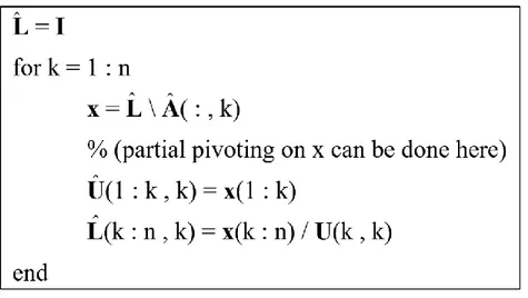
Figure 1.24 Nonzero pattern of x when solving Lx=b ... 43
Figure 1.25 ˆLi and ˆUi non-zero pattern allocation ... 44
Figure 1.26 Analysis of 1st column of matrix (1.68) ... 47
Figure 1.27 Analysis of 2nd column of matrix (1.68) ... 49
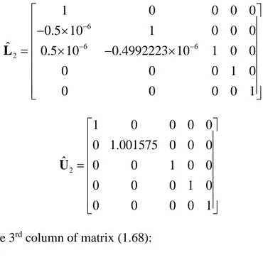
Figure 1.28 Analysis of 3rd column of matrix (1.68) ... 51
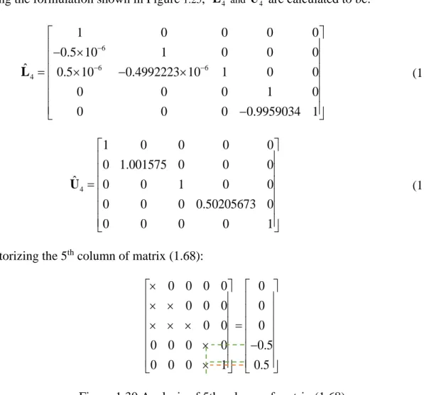
Figure 1.29 Analysis of 4th column of matrix (1.68) ... 53
Figure 1.30 Analysis of 5th column of matrix (1.68) ... 54
Figure 1.31 Matrix A elimination graph ... 60
Figure 1.32 1st elimination step of matrix A graph ... 61
Figure 1.33 2nd elimination step of matrix A graph ... 61
Figure 1.34 3rd elimination step of matrix A graph ... 62
Figure 1.35 4th elimination step of matrix A graph ... 62
Figure 1.36 Parallel implementation initialization phase ... 64
Figure 1.37 Parallel implementation Execution ... 65
Figure 2.1 Top view of Reluctance based transformer model case (Contributed by EDF) ... 68
Figure 2.2 Reluctance based transformer model case matrix sparsity pattern ... 69
Figure 2.3 Reluctance based transformer model case EMTP permutation for Matrix A ... 69
Figure 2.4 Reluctance based transformer model case KLU permutation of matrix A ... 70
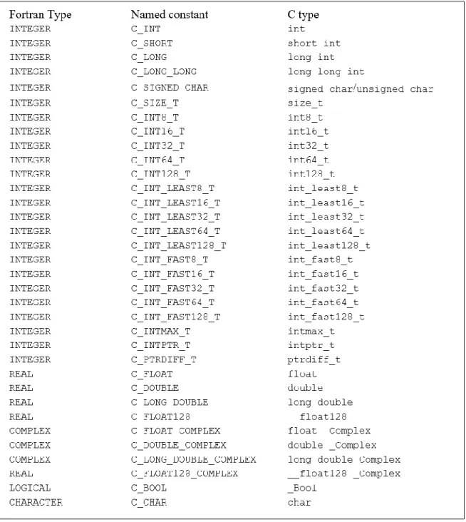
Figure 2.5 ISO_C_BINDING types declaration ... 72
Figure 2.6 KLU symbolic declaration using ISO_C_BINDING ... 73
Figure 2.7 ISO_C_BINDING functions declaration syntax ... 73
Figure 2.9 Pivot validity test flow chart ... 75
Figure 2.10 Cells to BTF blocks mapping ... 77
Figure 2.11 Sample circuit for demonstrating partial factorization ... 79
Figure 2.12 Shared memory OpenMP model ... 84
Figure 2.13 KLU_unit type declaration ... 85
Figure 2.14 Distributed model OpenMP design ... 87
Figure 3.1 Hydro-Quebec case top view ... 92
Figure 3.2 HQ-L matrix
A
before BTF ... 94Figure 3.3 HQ-L matrix
A
after BTF ... 94Figure 3.4 SMPEMT HQ-L Grid simulation time and gain ... 95
Figure 3.5 HQ-L Grid fault location ... 96
Figure 3.6 HQ-L grid line L7016 voltage drop - phase A ... 97
Figure 3.7 HQ-L grid Generator Mercier_A1 real power ... 97
Figure 3.8 HQ-L grid Generator Hydrocanyon_A real power ... 98
Figure 3.9 T0-Grid top view ... 99
Figure 3.10 T0-Grid matrix
A
before BTF ... 100Figure 3.11 T0-Grid matrix
A
after BTF ... 101Figure 3.12 SMPEMT T0-Grid simulation time and gain for DM model ... 101
Figure 3.13 T0-DM Grid fault location ... 102
Figure 3.14 Line ADAPA TO GOKCE voltage drop - phase A ... 103
Figure 3.15 Generator CAYIR TPP CAYIRHAN U1 real power ... 104
Figure 3.16 Generator CAYIR TPP CAYIRHAN U2 real power ... 104
Figure 3.18 T1-AVM Grid matrix
A
before BTF permutation. ... 106Figure 3.19 T1-AVM Grid matrix
A
after BTF permutation ... 107Figure 3.20 SMPEMT T1-Grid simulation time and gain for AVM model ... 108
Figure 3.21 T1-AVM fault location ... 109
Figure 3.22 T1-Grid line ADAPA TO CAYIR voltage drop - phase A ... 110
Figure 3.23 Generator CAYIR TPP CAYIRHAN U2 real power ... 110
Figure 3.24 T2-AVM Grid top view ... 112
Figure 3.25 T2-AVM Grid matrix A before BTF permutation ... 113
Figure 3.26 T2-AVM Grid matrix A after BTF permutation ... 113
Figure 3.27 SMPEMT T2-Grid simulation time and gain for AVM model ... 114
Figure 3.28 Line ADAPA_TO_CAYIR voltage drop - Phase A ... 115
Figure 3.29 SM CAYIR TPP CAYIRAN U2 real power ... 115
Figure 3.30 IEEE14-Grid matrix A before BTF permutation ... 117
Figure 3.31 IEEE14-Grid matrix A after BTF permutation ... 117
Figure 3.32 Line PI15 voltage drop - phase A ... 118
Figure 3.33 IEEE7000-Grid matrix A before BTF permutation ... 119
Figure 3.34 IEEE7000-Grid matrix A after BTF permutation ... 120
Figure 3.35 SMPEMT IEEE7000-Grid simulation time and gain ... 120
Figure 3.36 IEEE39-Grid top view ... 123
Figure 3.37 IEEE39-Grid matrix A before BTF permutation ... 124
Figure 3.38 IEEE39-Grid matrix A after BTF permutation ... 124
Figure 3.39 SMPEMT IEEE39-Grid simulation time and gain ... 125
Figure 3.41 Line 03-04 voltage drop - phase A ... 127
Figure 3.42 Power Plant 10 real power ... 127
Figure 3.43 Single line diagram of IEEE-118 Grid ... 129
Figure 3.44 IEEE118-Grid matrix A before BTF permutation ... 130
Figure 3.45 IEEE118-Grid matrix A after BTF permutation ... 130
Figure 3.46 SMPEMT IEEE118-Grid simulation time and gain ... 131
Figure 3.47 A network with a limiting block ... 133
LIST OF SYMBOLS AND ABBREVIATIONS
EMT: Electromagnetic transient
MANA: Modified augmented nodal analysis EMTP: Electromagnetic transient program BTF: Block triangular form
BDF: Block diagonal form
AMD: Approximate Minimum Degree
COLAMD: Column Approximate Minimum Degree A : Matrix with no permutation
ˆA: Matrix with BTF permutation CPU: Central processing unit GPU: Graphical processing unit TVMs: time-varying models
ITVM: iterative time-varying method CSC: Compressed Column Format CSR: Compressed Raw Format NNZ: non-zero element
NE: Network equations NM: Non-linear models TVM: Time-varying models BDF: Block diagonal Format HQ: Hydro-Quebec
FLCC: First left changed column FLDC: First left dynamic column
SMPEMT: Sparse matrix package for EMTs IBP: In block permutation
NFPO: Number of floating-point operations DFS: Depth first search
KLU-FF: KLU Full Factorization technique KLU-RF: KLU Re-Factorization technique
CHAPTER 1
INTRODUCTION
The circuit based electromagnetic transient (EMT) simulation approach is a powerful approach for studying power transmission and distribution grids. The range of applications of EMT-type tools varies from very fast transients to slower electromechanical transients. Typical studies include switching transients, lighting transients, HVDC transmission, wind generation and electromechanical transients from small to very large-scale systems. EMT simulation is also used in the design and sizing of power network components such as insulation levels and energy absorption capabilities. EMT-type simulation tools are subdivided into two main categories: off-line and real-time. The main goal of performing off-off-line is to perform simulations on generic computers that are easily available to engineers. Real-time simulation tools are capable of generating results in synchronism with a real-time clock. Such tools have the advantage of being capable of interfacing with physical devices and maintaining data exchanges within the real-time clock. The capability to compute and interface within real-time, imposes important restrictions on the design of such tools. Current off-line EMT-type simulation tools remain more accurate than the real-time counterparts. They are also capable of solving much larger power grids and maintain higher accuracy. Nevertheless, research on the acceleration of off-line tools is also applicable to the eventual acceleration of real-time tools. Convergence of these tools into a single environment is inevitable in the near future.
Instead of using EMT-type tools in time-domain, it is also possible to simulate large power grids through phasor-domain computations. Phasor-domain tools are also referred to as transient stability (TS) tools. The TS approach can be very fast, especially when solving very large-scale systems, but it suffers from important accuracy issues. This is becoming nowadays an important issue with the increased usage of power electronics-based components (wind generation, HVDC, photovoltaics...) in modern power systems. In fact, in more and more applications, the much more accurate EMT-type methods and models are called to replace the usage of TS-type simulation and modeling. This trend will subsist, and EMT-type tools will receive wider and wider acceptance in practical applications, especially when they become capable of much higher efficiency for networks of very large dimensions.
This thesis presents the implementation of a parallel sparse matrix solver used for improving the computational speed of EMT-type tools. The new approach contributes in enhancing the overall
quality of EMT simulation by reducing the simulation time while maintaining the simulation accuracy and reliability. Unlike other solvers published in the literature that are demonstrated by repeating a small network multiple number of times, the proposed approach can be generalized and is valid on any power system network. The proposed new method is also capable of automatically parallelizing networks of arbitrary topologies without any user intervention.
The new method presented in this thesis is based on the KLU sparse matrix solver which is currently the most suitable for circuit-based simulation methods [1]. The solver is programmed using parallelization algorithm that can automatically detect independent parts of the sparse matrix separated by the natural decoupling available in transmission line/cable models. This decoupling technique can be detected without any user intervention and pre-determination of different subnetworks.
Due to the iterative process required for solving nonlinearities in various models, this thesis also contributes modifications into the KLU solver for improving its performance when repetitive matrix refactorizations are requested.
The proposed new approach is demonstrated using an EMT-type software (i.e EMTP) that uses a fully iterative solution method for all nonlinear models [2]. It remains however applicable to any EMT-type software tool that uses sparse matrices. A modular sparse matrix package can be replaced easily by the package elaborated in this thesis.
1.1 Thesis Outline
This thesis is divided into four chapters that are summarized below. Chapter 1: Introduction
This chapter introduces the concept of EMT simulation and the modified-augmented nodal analysis (MANA) approach used in the EMTP simulation package to form its sparse matrix [3]. This approach is explained in detail and illustrated with an example. In addition, different sparse solvers are introduced in this chapter including the minimum degree ordering (MDO) based approach used in EMTP [4]. These solvers are used and compared to select the fastest package and enhance it as it will be demonstrated in the following sections.
In the second part of this chapter, different methods such as BTF, MDO, SSN and Compensation theory are introduced as well.
The last part of this chapter discusses different threading algorithms used in implemented the multi-threaded sparse solver used in this thesis.
Chapter 2: Implementation of Sparse Matrix Package for EMTs
In this chapter the approaches used to accelerate the simulation process are explained and the implementation of a new sparse solver that is customized only for EMT-type simulations is introduced and explained. In addition, a comparison between the new sparse solver and other already existing ones is presented and discussed.
Chapter3: Test Results
In this chapter, different benchmarks used in the process of validating the new sparse solver will be presented. These test cases consist of real and existing networks with complex models, including nonlinearities and power-electronics converters for wind generator applications. Each network’s topology is described with related matrices and complexity level. Computational timings are used to demonstrate the advantages of the approach presented in this thesis.
The results of each test case are analyzed and studied. The acceleration rate (gain) for each case will be looked at in depth and compared with other cases. Observations and limitations will be address herein as well.
Chapter 4: Conclusion and Future work
This chapter provides a quick summary of the overall work done throughout this PhD work and it highlights the main milestones that were achieved during this project. In addition, it provides recommended future work.
1.2 Contributions
In this thesis the multithreading approach used for programming a parallel sparse solver is based on the OpenMP standard and the use of distributed memory design. Thanks to this design an efficient parallel solution is achieved, and the effect of overhead timings is kept at minimum. This parallel model design minimizes shared memory between different threads and allows each thread to store its own data on its own designated memory. This approach makes it easier for all threads to fetch and write data to memory without the need to communicate with the master thread or any other threads for that matter.
Another noticeable contribution in this thesis is the fact that the proposed method is tested on realistic large-scale network benchmarks. Parallelization is achieved without any user intervention. Such practical networks allow to derive more realistic conclusions on the potential gains in EMT-type solver parallelization.
1.3 Literature review
The computing time reduction for the simulation of electromagnetic transients[2][5] (EMTs) is a crucial research topic. The EMT-type[5] simulation methods are circuit based and can use very accurate models for an extended frequency range of power system phenomena. This qualifies them as being of wideband type. In fact, the EMT approach is applicable to both slower electromechanical transients and much faster electromagnetic transients. The computation of electromechanical transients can be achieved with EMT-type solvers for very large networks [6] and requires significant computing time when compared to phasor-domain approaches, but even for smaller networks, the computing time can become a key factor due to numerical integration time-step constraints or model complexity level. More and more challenging simulation cases are created for studying modern power systems, those include, for example, HVDC systems and wind generation[7].
There are several techniques for improving computational performance in EMT-type solvers. Such techniques include improvements in model performance using, for example, average-value models[8] for power-electronics based systems or circuit reduction [9]. Network reduction can be also achieved using frequency domain fitting[10], or through dynamic equivalents[11]. Other approaches include usage of multiple time-steps[12], waveform relaxation [13] and combinations of different methods [14]. An important problem in network solution parallelization methods, such as[15], is that user intervention is required for setting the network separation locations and task scheduling. The user should be aware of the case details in order to best allocate the separation locations and optimize the performance of the parallel solution. It is also necessary to program network topology analysis and, in some methods such as in [16], analysis can be used for automatic task scheduling.
A more direct path towards computational speed improvement in EMT-type numerical methods is through efficient sparse matrix solvers and parallelization. This chapter introduces different types of sparse solvers used in general circuit analysis. These solvers are currently implemented in different simulation tools and each has its own advantages and disadvantages. Moreover, parallel computation concept will be discussed, and different parallel programming techniques will be introduced. These techniques will be used in this thesis to implement the EMT customized sparse
solver. In addition, different ordering techniques will be discussed such as AMD, COLAMD, BTF and METIS.
This work targets off-line simulation methods and presents CPU-based parallelization for conventional multi-core computers using a sparse matrix solver, named KLU [1].
1.3.1 Modified-Augmented-Nodal Analysis (MANA)
The modified-augmented-nodal analysis (MANA) method is briefly recalled in this section. The traditional approach for the formulation of main network equation is based on nodal analysis. The network admittance matrix Y is used for computing the sum of currents entering each n electrical node and the following equation results from classical nodal analysis.
n n n
Y v = i (1.1) where, v is the vector of node voltages and the members of n i holds the sum of currents entering n each node. It is assumed that the network has a ground node at zero voltage which is not included in (1.1) . Since the network may contain voltage sources (known node voltages), equation (1.1) must be normally partitioned to keep only the unknown voltages on the left hand side
' ' ' n ns n n sn ss s s Y Y v i = Y Y v i (1.2) = − n n n ns s Y v i Y v (1.3) where ' n
Y is the coefficient matrix of unknown node voltages v , n ' n
i holds the sum of currents entering nodes with unknown voltage, YnsY and relates to known voltagesn v . It is noticed thats
T '
n n s
v = v v [20].
Equation (1.3) has several limitations. It does not allow, for example, to model branch relations instead of nodal relations and it assumes that every network model has an admittance matrix representation, which is not possible in many cases. This is where the modified augmented nodal analysis comes into play. The MANA formulation method [20][21][22] is a relatively new approach to formulate network equations. This method offers several advantages [3] over classical
nodal analysis. Its formulation is recalled here to relate to material presented in the following sections. In MANA the system of equations is generic and can use different types of unknowns in addition to voltage. Equation (1.3) is augmented to include generic device equations and the complete system of network equations can be rewritten in the more generic form as seen in (1.4).
N N N
A x = b (1.4) In this equationYnAN, x contains both unknown voltage and current quantities and N b N contains known current and voltage quantities. The matrix A is not necessarily symmetric and it N is possible to directly accommodate non-symmetric model equations. Equation (1.4) can be written explicitly as n c n n r d x x Y A v i A A i v = (1.5) where the matrices A , r A and c A (augmented portion, row, column and diagonal coefficients) d are used to enter network model equations which are not or cannot be included in Y , n i is the x vector of unknown currents in device models, v is the vector of known voltages, x x = vN
n ix
T and bN =
in vx
T[23].It is emphasized that the system in (1.5) is non-symmetric and can also accommodate generic equations, such as
1 k 2 m 3x 4 y ... z
k v +k v +k i +k i + =b (1.6) Where the terms on the left contribute coefficients (kj ) into the A matrix for voltage (vj) and current (ij) unknowns, and bz is a cell in the b vector. This equation allows integrating directly source and switching equations. For example, an ideal switch can be represented by
0 k m s km
kv −kv −k i = (1.7)
When the ideal switch is in closed position, k =1 andk =s 0 . When the ideal switch is open, k =0
high and low resistance values. Other, models, such as ideal transformers with tap control can be easily accommodated [3].
Single phase and three-phase transformers can be built in EMTP using the ideal transformer unit shown in Figure 1.1. It consists of dependent voltage and current sources. The secondary branch equation is given by
2 2 1 1 0
k m k m
v −v −gv +gv = (1.8) Where, g is the transformation ratio. This equation contributes its own row into the matrix A r whereas the matrix A contains the transposed version of that row. It is possible to extend to c multiple secondary windings using parallel connected current sources on the primary side and series connected voltage sources on the secondary side. Leakage losses and the magnetization branch are added externally to the ideal transformer nodes.
Three-legged core-form transformer models or any other types can be included using coupled leakage matrices and magnetization branches.
Figure 1.1 Ideal transformer model unit
The MANA formulation (1.4) is completely generic and can easily accommodate the juxtaposition of arbitrary component models in arbitrary network topologies with any number of wires and nodes. It is not limited to the usage of the unknown variables presented in (1.5) and can be augmented to include different types of unknown and known variables. The MANA formulation is conceptually simple to realize and program [23][24].
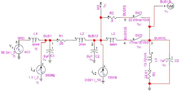
In order to provide a better understanding of the MANA formulation, the following example illustrates a simple circuit with its MANA formulation. Figure 1.2 illustrates the example circuit
1
k
k
2
1
m
m
2
2 2 k m g i − 2 2 k m i(
k1 m1)
g v −v+
-structure with all its components names and ratings. The analysis of this circuit starts by forming the submatrix Y that contains the admittance matrix of the MANA main matrix. n
Figure 1.2 MANA Formulation Example
In order to find the time domain system of equations using the MANA formulation, the linear components of the circuit above (i.e inductors and capacitors) need to be discretized for a given integration time step tusing a numerical integration method. Although any discretization rule can be used, the trapezoidal rule technique has been used herein to discretize nonlinear model of the circuit into linear representation. The inductor equation shown in (1.9) is discretized into a linear format shown in (1.10), this discretization allow to model the inductor as shown in Figure 1.3. Similarly, the capacitor equation can be discretized in a similar fashion as well.
km km di v L dt = (1.9) 2 2 t t t t t t km km km km t t i v v i L L − − = + + (1.10)
Figure 1.3 Discretized inductance model for time domain MANA solution
Equation (1.11) shows the MANA formulation of the circuit shown in Figure 1.2. The equation of each node has been written by replacing the inductors and capacitors connected to it by their discretized model. Node 1 for example (which represents BUS 1 in Figure 1.2), has L, C and RL branches connected to it in addition to the current source i . Hence, replacing the L, C and RL s1
branches with their discretized model produces the node junction shown in Figure 1.4 where R1, R3 and R4 represent the resistors in the discretized model of L1, C1 and L2 respectively.
s1 h61 h12 1 11 12 16 2 21 22 24 3 33 4 42 44 5 6 61 66 Vs SW1 SW2 i +i -i -v y y 0 0 0 y 0 0 0 v y y 0 y -2 0 0 0 0 v 0 0 y 0 0 0 0 0 0 v 0 y 0 y 0 0 0 0 0 v = 0 -2 0 0 2 0 0 0 0 v y 0 0 0 0 y 1 0 0 i 0 0 0 0 0 1 0 0 0 i 0 0 1 0 1 0 0 1 0 i 0 0 0 0 0 0 0 0 1 − 1 2 h10 s2 h12 h20 h24 h30 h30 h24 h61 s i i +i -i -i -i -i i 0 -i v 0 0 (1.11)
Figure 1.4 BUS1 branches discretized model
Hence, the value of y shown in equation (1.11) is the summation of R1, R2, R3 and R4 11
admittances that can be calculated using the following equation: 6 11 3 3 2 0.8 10 1 2 2 10 2 6 10 0.05 t y t t − − − = + + +
In a similar manner all quantities in the Y part of the MANA matrix can be found as follows: n
12 3 1 2 2 10 0.05 y t − = − + 16 3 2 6 10 t y = − − 22 11 1 0.5 y = y + 21 12 y = y 24 42 3 2 6 10 t y = y = − − 6 33 3 2 1 10 1 2 19.72 10 22.61 y t t − − = + + 44 24 y = −y BUS1 + R1 + R2 + R4 + i61 + R3 + is1 + i10 + i1 2
66 16
y = −y
61 16
y = y
The terms on the right of (1.11) are the contributions from independent current sources and history current sources resulting from component discretization (inductances and capacitances).
In the current project, EMT simulation is solved at each time step after updating A for switches position changes, transformer tap changes or any other modifications in model equations (including nonlinear devices). For nonlinear models (NMs), the NEs must be solved iteratively to achieve an accurate simultaneous solution. This is done by linearizing each model at each operating point and solving iteratively [3]. Model linearization results into a Norton equivalent with the Norton resistance contributing changes into the A matrix and the Norton current contributing updates into the b vector.
It means that at each time-point it is necessary to resolve (1.11) iteratively until convergence for all nonlinear models is achieved.
For time-varying models (TVMs), such as switches or transformer tap positions, it is also possible to update A iteratively without advancing to the next time-point. This accuracy option, marked as iterative time-varying method (ITVM), allows achieving a simultaneous solution for the determination of all changes and dependencies between models at the same time-point. This process also includes the sequential re-calculation of control system equations [3].
1.4 Parallelization and network tearing
In order to be able to solve power systems in parallel, the network system of equations needs to be subdivided into multiple subnetworks. This division process allows distributing different parts of the network on different CPU cores and solving these subnetworks independently. Several schemes can be used to achieve this goal. A list of known methods is presented in this section.
1.4.1 Block Triangular Format (BTF)
The block triangular formulation of a matrix is an approach specialized in permuting the matrix by putting as much non-zero elements of the matrix along the diagonal [25]. This reordering allows
the flexibility of partially decoupling the matrix into different submatrices and allows the solving of these submatrices separately. Figure 1.5 shows a generic representation of the block triangular format with blocks A aligned along the diagonal and some off-diagonal elements ii Aij. These off
diagonal blocks/elements arise due to light links between different parts of the matrix such as block 11
A and A that are linked through 33 A block, and 13 A and 22 A that are linked through 55 A 25 block. In this thesis all cases used have no off-diagonal elements in them thanks to the time domain decoupling produced by transmission lines. Although, the parallelization of matrices shown in Figure 1.5 is still feasible, it involves more restrictions and complications.
Figure 1.5 An example of a matrix in BTF form
Another type of block triangular form that is more interesting for parallelization and mainly used herein, is the type where there are no off diagonal blocks/elements. This type of format is called block diagonal form BDF since all matrices elements are aligned along the matrix diagonal and the rest are zeros as can be seen in Figure 1.6 [25].
In order to transform a matrix into the BTF form, the KLU package uses a special technique that is based on Duff and Reid’s algorithm [25]. This algorithm finds any matrix BTF form (if applicable) by finding all strongly connected vertices of the matrix. It starts by preparing the matrix adjacency graph which guides the algorithm by moving from one graph vertex to another. Then a depth first search is launched starting from a random vertex and tries to visit/reach the maximum number of graph vertices of which there exists a path.
The design of KLU BTF algorithm uses a user-built stack that keeps track of all visited and unvisited vertices and avoids many run time errors such as stack over flow and memory shortage. The algorithm uses depth first search (DFS) topology that is based on a recursive algorithm to find all possible strongly connected vertices in the graph and keeps track of all visited and non-visited vertices. Once all connected vertices are labeled as visited, those vertices (nodes) form a block in the BTF form and the DFS algorithm begins again starting from an arbitrary non-visited vertex. The vertex graphs are explored and all efforts to try all combinations of connections is exhausted. The following example gives a better visualization of how the BTF algorithm calculates strongly connected regions of the matrix. It is noticed here that the transmission line models are of distributed parameter type. In fact, any such model, either with constant parameters or with frequency dependent parameters, offers an important property for parallelization. The line (or cable) model provides a delay between its left (k-side)) and right (m-side) hand sides. This means that the k-side network can be solved completely independently from the m-side network without any approximation. This well-known property is the key ingredient used in this thesis for delivering parallelization. Nevertheless, the independent subnetworks created by transmission lines, must be found automatically.
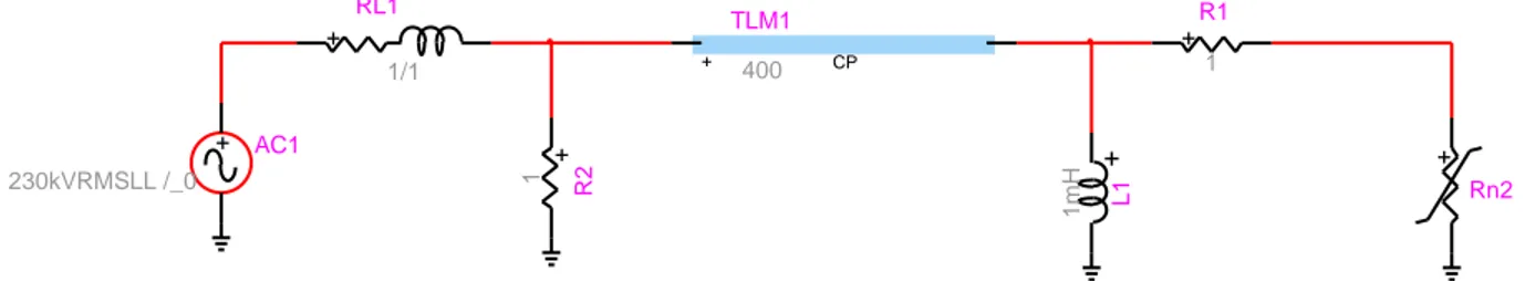
The sparsity pattern of the matrix of the network shown in Figure 1.7 is presented in Figure 1.8, and the BTF version of this matrix is presented in Figure 1.9. The BTF method can automatically derive the block-diagonal (BD) without any user intervention as long as the case has at least one transmission line implemented in it.
Figure 1.7 BTF format test case
Figure 1.8 Sparsity pattern of matrix A of circuit shown in Figure 1.7
Figure 1.9 BTF Sparsity pattern of matrix A of circuit shown in Figure 1.7 + AC1 230kVRMSLL /_0 + RL1 1/1 + R2 1 + Rn1 CP + TLM1 400 + R1 1 + L1 1mH
In order to facilitate the differentiation between a BTF ordered matrix with a non-ordered matrix, the “hat” symbol is used from now on to represent all BTF ordered matrices (i.e ˆA). In addition, the second digit in the BTF block index will be dropped due to the fact that all cases used herein have no off-diagonal blocks and both digits used to refer to a BTF block in this case are the same (i.e ˆAi refers to block i in the BTF ordered matrix ˆA). The BTF ordering is similar to graph traversal ordering that is based on a depth first algorithm to find all decoupled subnetworks and used in [16]. This ordering tries first to decouple the network based on the presence of the existing transmission lines and detect each subnetwork by the end of traversal, and at the same time they apply a heuristic calculation on the time cost for each component type (R, machine, inductance, etc...) in the subnetwork to make the simulation fit to real time simulation. Based on the execution cost, it can decide to join several subnetwork in one cpu and put this in one matrix if the resolution will fit in one step.
In KLU solver package, the BTF ordering is followed by another ordering that aims at reducing the ˆLi and ˆUi matrices fill-in. There are three ordering techniques that are already implemented in KLU package which are AMD, COLAMD and a user pre-defined ordering. This step plays a major role in reducing computational load during KLU numerical solution by reducing the number of floating-point operations required to solve the system. This type of ordering will be discussed in the coming sections.
1.4.2 METIS
METIS is an efficient algorithm that allows the partitioning of a matrix into multiple submatrices that are either independent of each other or share elements with other submatrices with all shared elements aligned along the submatrices boarders. An advantage of METIS is the feasibility of increasing the degree of parallelism with the existence of only one partitioned matrix in the system. METIS is specialized in partitioning large-scale irregular graphs or meshes and providing a permutation that provides an efficient partitioning as well as a reduction of fill-in of ˆLi and ˆUi factors [26].
Unlike other traditional ordering techniques that work on the graph directly to provide a portioning by one step operation, and hence provide a low quality and less efficient partitioning, METIS is
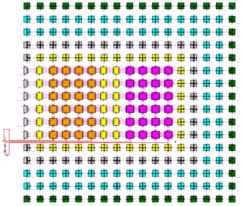
based on multi-level graph partitioning technique that adopts a totally different technique that works on the graph and reduces the size of the graph as much as possible, by collapsing graph vertices and edges and partitioning the small graph and re-ordering it to produce the partitioning of the original graph [26]. Figure 1.10 shows matrix A of the IEEE1138 bus system ordered by METIS algorithm.
Figure 1.10 IEEE-1138 network ordered by METIS
Not only METIS can provide a high-quality portioning over other ordering techniques, it is considered one of the fastest ordering techniques that can provide its partitioning results in one or two orders faster that other traditional algorithms. Moreover, METIS ordering contributes in reducing the fill-in of ˆLi and ˆUi factors without the need of using other techniques to do this task. METIS has the ability to produce more blocks along the diagonal compared to BTF. This phenomenon is due to the fact that METIS does not require a complete decoupling of blocks like BTF, but rather it can still reorder a block (that BTF was not able to partition) into sub-blocks and align all shared elements between these sub-blocks along the matrix or block border.
However, given the types of problems this thesis deals with, and the fact that BTF blocks are totally independent of each other, the use of METIS becomes less significant for cases that have multiple transmission lines that allow decoupling the case in time domain into relatively small independent regions. The importance of this ordering technique arises when a large-scale case with no
transmission line in its structure (or have very few of them) is being studied. Using Metis in this case helps introduce some degree of parallelization into the solution. In addition, this partitioning technique can help reduce the effect of large limiting blocks that prevent parallel simulation as will be seen in chapter 3. In addition, different fill-in reduction techniques that were tested herein (such as AMD) were found to be more efficient and produce around 15% less fill-in compared to METIS.
1.4.3 SSN and MANA
Another parallelization approach can be achieved through the combination nodal or MANA equations with state-space equations. This approach, name state-space nodal (SSN), is explained in [27]. The basic principle is that the network is separated (cutting) into state-space groups that are solved independently in parallel and combined through MANA equations.
Although the SSN method is perfectly accurate, it has two drawbacks. First the network separation locations must be determined manually. Another problem is that the usage of state-space equations is typically inappropriate for solving large scale grids. Other complications arise when the state-space equations must be reformulated for nonlinear models and time-varying models.
1.4.4 Scotch
Scotch [28] is yet another sparse matrix package that focuses on solving graph theory-based problems using divide and conquer approach. It is used in wide range of applications and not limited to electrical or power circuit problems, this package is based mainly on nested dissection approach to permute the application sparse matrix into a format that allows certain degree of parallelization. The nested dissection starts by forming the matrix undirected graph in which the vertices represent rows and columns of the matrix, and an edge/connection in the graph represents a nonzero entry in the sparse matrix. Once the graph is formed, the nested dissection algorithm uses a divide and conquer strategy on the graph in order to remove a set of vertices to result in two new graphs that are independent of each other. This algorithm uses a recursive technique that partitions the graph into subgraphs by selecting barriers or separators that consist of small set of graph vertices. The removal of these separators creates independent subgraphs. Applying factorization and solving the matrix parts that represent the new sub-graphs can be done
independently and in parallel. The results of the two new graphs can then be combined to find the overall matrix results.
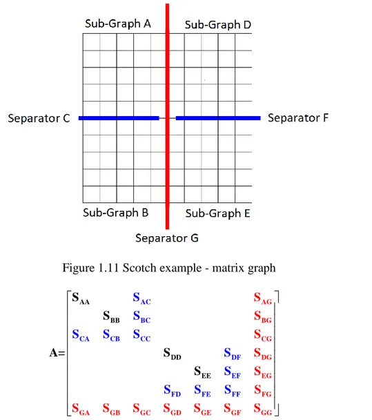
In order to better understand the nested dissection ordering, the following matrix shown in Figure 1.11 gives an example of a matrix graph (mesh) that is ordered by nested dissection. In this figure, the graph is partitioned into four subgraphs (A, B, D and E) by three different separators (C, F and G). The matrix shown in equation (1.12) is a representation of the matrix after being reordered.
Figure 1.11 Scotch example - matrix graph
AC BC CA CB CC DF EF FD AG BG CG DG EG FG F GA GB GC GD GE G G AA BB DD EE F F G E F S S A S S S S S S S S S S S S S S S S S S S S S S S S = S (1.12)
Equation (1.12) shows the matrix after being ordered by nested dissection. All black elements in the matrix represent sub-graphs created after adding the separators, and all blue and red elements represent elements that are located across the separators (C, F and G) and they are linking different black blocks together.
Comparing this ordering technique with other ordering techniques, it is found that the nested dissection ordering is only applied to symmetric matrices, and that is a condition that can’t be met and guaranteed in many EMT simulation tools including EMTP.
1.4.5 Bordered Block Diagonal matrix
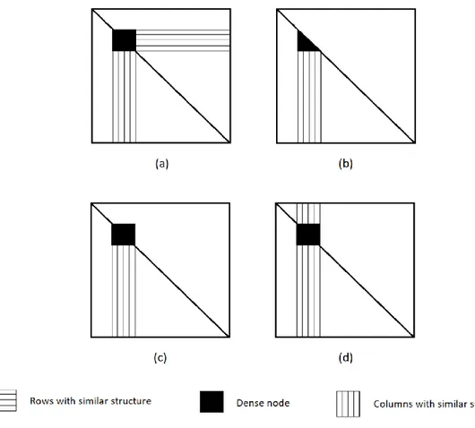
This ordering scheme is a methodology that permutes the power system network matrix A into a doubly bordered block diagonal (DBBD) or a single bordered block diagonal (SBBD). Figure 1.12 shows the typical structure of a DBBD permuted matrix [29].
Figure 1.12 Doubly bordered block diagonal (DBBD)
It can be seen from Figure 1.12 that a doubly bordered block diagonal form is similar to a block upper triangular form but has non-zeros on the sub diagonal region. These nonzero elements found in the lower section of the diagonal form a horizontal strip resembling a border. The same thing applies for nonzero elements above the diagonal, these elements form a vertical strip that resemble a vertical border. Many ordering techniques can be used to produce DBBD permuted matrix such as METIS and nested dissection [26].
Generically speaking, when a complete network or a network portion does not contain delay-based transmission line models, it will not be possible to create a BD matrix for its equations. It can be demonstrated that for such cases, it is possible to derive a BBD matrix as seen in following compensation theory section.
1.4.6 Compensation Theory
The Compensation method theory is presented in [31]-[33] and it was used in [34]. The application described in [34] is for the solution of nonlinear models in an EMT-type code. The limitations that this method may encounter for solving nonlinearities, or in general, are described in [35]. It is
shown in [35] that the compensation method although very powerful, is not conformable to the topological proper-tree and therefore has topological limitations. The hybrid analysis method [36]-[38] has been shown in [40] to be more general than the Compensation algorithm. The work in [35][39] relates the more general hybrid analysis to the Compensation method.
Despite the limitations of the Compensation method for solving nonlinear systems, it will be used below to demonstrate how it links to other methods in the literature and how it can be used to decouple networks when transmission line delay-based decoupling is not possible.
The basic idea of the Compensation method is illustrated in Figure 1.13. In this figure the dash line shows cutting through wires. It is assumed that a linear or nonlinear network N2 is connected to network N1 through one or more wires. In some publications [34] it is assumed that N2 can contain only (one type of) nonlinear component, but N2 can actually contain any number of nonlinear components and it fact it can contain complete arbitrary (except for cases explained in [35]) networks. In the following, it will be assumed that N2 is actually a grid with any number of components. N2 can be purely linear.
Figure 1.13 Separation of two networks using the compensation method
Let us assume the wires (ˆn wires) connecting N2 to N1 are connected to a set of nodes Nˆ in N1. It can be written that for any time-point solution
ˆ ˆ ˆ final N N N = + v v v (1.13) where vNˆ is the solution vector of node voltages for N1 when it is disconnected from N2, vNˆ is the solution found from the contributions of currents entering N1 through ˆn wires and vNfinalˆ is the final solution through the superposition theorem. In this presentation, it is assumed that N1 does
not contain any nonlinearities, whereas N2 may contain nonlinear components that require iterations for an accurate solution. It can be further shown that
ˆ N =
v Z i (1.14) where Z is an impedance matrix relating the currents entering the set of nodes Nˆ to the contributions on voltages vNˆ. By using an incidence matrix, the branch voltages in N2 are related by ˆ ˆT final n N = v A v (1.15) where Aˆn is the nodal incidence matrix for the nodes in N2. If all the ˆn wires are connecting from node to ground, then Aˆn becomes unitary and diagonal. By combining equation (1.13), (1.14) and (1.15) ˆ ˆ T th n = + v v A Z i (1.16) where vˆth is the vector of Thevenin voltages as found from N1. It is apparent that the Thevenin
impedance matrix Zˆth is given by
ˆ ˆ T th= n Z A Z (1.17) and consequently ˆ ˆth th = + v v Z i (1.18) Finally, it is noted that the currents i and voltages v are related through a function Φ that could
be linear or nonlinear:
(
,)
=0Φ v i (1.19) If Φ is nonlinear then (1.18) must be solved using iterations and the Newton method.
The vector vˆth is time-dependent and must be found at each time-point solution. The matrix Zˆth
may also have time-dependency due to switching devices in N1.
In Figure 1.13 it is assumed that N1 includes coupled (no delay-based transmission lines) networks. It is however possible that N1 contains decoupled networks or wires are used to connect separate networks. Let us assume that there are now two networks in N1 and N2 that are connected together
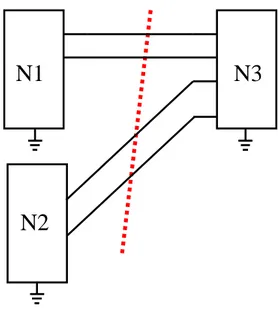
using the circuit of network N3. In that case the new representation of relations between networks is shown in Figure 1.14.
Figure 1.14 Two networks N1 and N2 connected through wires in network N3. The MANA formulation of network equations for Figure 1.14 is given by
= k m 1 c 1 1 2 c 2 2 3 3 k m d A 0 S x b 0 A S x b x b S S S (1.20)
In the above system, A1 is the matrix of N1, A2 is the matrix of N2, the Smatrices are the connecting matrices from network N3. It is possible that some off-diagonal S matrices are nullified due to disconnection between N1 and N2. Equation (1.20) is generic and allows N3 to contain longitudinal impedances, but for the following text and without any lack of generality, it is assumed that the impedances in N3 are simply zero, meaning that N1 and N2 are interconnected through ideal wires. For ideal wires, equation (1.20) becomes
T T = 1 k 1 1 2 m 2 2 3 k m A 0 S x b 0 A S x b x 0 S S 0 (1.21)
The Compensation based solution of (1.20) (or (1.21)) can proceed as follows at each solution time-point. First it is necessary to solve with switches open (cutting the wires) by using
N1
N3
= 1 1 1 2 2 2 3 A 0 0 x b 0 A 0 x b 0 0 1 i 0 (1.22)
In this way the unknowns x1 and x2 are found before compensation and x3=i3 for the wire currents (zero in this solution stage). From the found vectors x1 and x2 it is possible to directly extract the network Thevenin voltages vˆth1 and vˆth2, respectively. Then using current injection
method in b1 and b2 for each network, it is possible to derive the Thevenin impedances. In the following equations the double-primed vectors signify the current injection method for finding the Thevenin impedances Zˆth1 and Zˆth2 (column-by-column process):
= = 1 1 1 2 2 2 A x b A x b (1.23) At this stage it is possible to solve for the wire currents i3 with
ˆ ˆ ˆ ˆ
th th th th
+ = −
Z 1 Z 2i3 v 1 v 2 (1.24) The above relation is illustrated in Figure 1.15 and it is assumed that the wire currents are oriented from left to right. It is also assumed that the coefficient matrix resulting in (1.24) is not singular.
Figure 1.15 Compensation based equivalent of network in Figure 1.14.
After solving for i3 in (1.24), it is now possible to solve for the contributions (x1 and x2) of i3 on N1 and N2: = − = − 1 1 k 3 2 2 m 3 A x S i A x S i (1.25) Finally, we can apply superposition (compensation) to find
+ + + +
= + = + 1 1 1 2 2 2 x x x x x x (1.26) The above procedure must be applied at each solution time-point. Any number of networks can be used and interconnected using wires (or impedances). Equations (1.23) and (1.25) can be solved in parallel. If there is any topological change in N1 or/and N2, it is necessary to recalculate Zˆth1 or/and
ˆ th2
Z . This is an important limitation and can become computationally very intensive with power-electronics based systems.
The above solution steps can be explained and performed differently. Equation (1.21) can be rewritten as follows ˆ ˆ ˆ = 1 1 1 2 2 2 3 3 3 b 1 0 S x 0 1 S x b 0 0 S i b (1.27) with 1 − = 1 1 k S A S (1.28) 1 ˆ = − 1 1 1 b A b (1.29) 1 − = 2 2 m S A S (1.30) 1 ˆ = − 2 2 2 b A b (1.31) T T = + 3 k 1 m 2 S S S S S (1.32) ˆ = Tˆ + Tˆ 3 k 1 m 2 b S b S b (1.33) From (1.24) and (1.32) it is seen that
ˆ ˆ th th = 1+ 2 3
S Z Z (1.34) From (1.24) and (1.33) it is apparent that
ˆ ˆ ˆ
th th = 1− 2 3
b v v (1.35) because bˆ1 is actually x1 in (1.22). The same applies for bˆ2 and x2. It is noted that the coefficients of STm are negative (ideal switch equations) and that explains the corresponding negative sign in (1.35). Finally, it is clear from (1.27), (1.25) and (1.26) that
1 1 − − = − + = + 1 1 k 3 1 1 1 1 x A S i A b x x (1.36)
1 1 − − = − + = + 2 2 m 3 2 2 2 2 x A S i A b x x (1.37) The approach derived with (1.27) is actually called MATE (Multi Area Thevenin Equivalent) [40][41]. As proven above with (1.36) and (1.37), and contrary to what is written in the literature, MATE is not a new theory or approach, it is in fact the Compensation method that was available in the literature much before!
The formulation of (1.20) indicates that if it is possible to find the bordered-block-diagonal matrix of a network, then it is possible to solve it in parallel even when distributed-parameter lines are not available. That solution uses the Compensation method (or MATE). Any number of networks can be separated (cut) and solved. The above illustration was made for two networks N1 and N2. But there is a fundamental flaw in this approach. In a typical network, the networks N1 and N2 may encounter topological changes and require recalculating S3 in (1.34), which is computationally inefficient and even catastrophic if repetitive switching occurs due to power-electronics converters, for example. Moreover, all of the above is assuming linear networks and becomes inapplicable for practical problems with nonlinearities. It is possible in theory to extend the above Compensation based network tearing to include nonlinearities, but that may result into significant computational inefficiencies and annihilate the gains due to parallelization.
As a final demonstration, one can notice that the presentation given for (1.27) is simply the symbolic solution of (1.21). The steps are written here for convenience:
ˆ = 3 3 3 S i b (1.38) ˆ = − + 1 1 3 1 x S i b (1.39) ˆ = − + 2 2 3 2 x S i b (1.40) The solution order is
1. solve in parallel: equation (1.29) for bˆ1 and (1.31) for bˆ2
2. solve for bˆ3 with (1.35) (the two parts of this equations can be calculated in parallel and then combined).
3. use (1.38) to find i3