Experiences in multiyear combined state-parameter estimation with an ecosystem model of the North Atlantic and Arctic Oceans using the Ensemble Kalman Filter

(1)

To link to this article :

DOI : 10.1016/j.jmarsys.2015.07.004

URL :

http://dx.doi.org/10.1016/j.jmarsys.2015.07.004

To cite this version :

Simon, Ehouarn and Samuelsen, Annette and

Bertino, Laurent and Mouysset, Sandrine Experiences in multiyear

combined state-parameter estimation with an ecosystem model of the

North Atlantic and Arctic Oceans using the Ensemble Kalman Filter.

(2015) Journal of Marine Systems, vol. 152. pp. 1-17. ISSN 0924-7963

O

pen

A

rchive

T

OULOUSE

A

rchive

O

uverte (

OATAO

)

OATAO is an open access repository that collects the work of Toulouse researchers and

makes it freely available over the web where possible.

This is an author-deposited version published in :

http://oatao.univ-toulouse.fr/

Eprints ID : 15387

Any correspondence concerning this service should be sent to the repository

administrator:

staff-oatao@listes-diff.inp-toulouse.fr

(2)

Experiences in multiyear combined state–parameter estimation with an

ecosystem model of the North Atlantic and Arctic Oceans using the

Ensemble Kalman Filter

Ehouarn Simon

a,

⁎

_{, Annette Samuelsen}

b,c

_{, Laurent Bertino}

b

_{, Sandrine Mouysset}

d

a_{Université de Toulouse, INP, IRIT, 2 rue Camichel, BP 7122, 31071 Toulouse Cedex 7, France}

b_{Nansen Environmental and Remote Sensing Center, Thormøhlensgate 47, 5006 Bergen, Norway}

c_{Hjort Center for Marine Ecosystem Dynamics, Thormøhlensgate 47, 5006 Bergen, Norway}

d_{Université de Toulouse, UPS, IRIT, 2 rue Camichel, BP 7122, 31071 Toulouse Cedex 7, France}

a b s t r a c t

A sequence of one-year combined state–parameter estimation experiments has been conducted in a North Atlantic and Arctic Ocean configuration of the coupled physical–biogeochemical model HYCOM-NORWECOM over the period 2007–2010. The aim is to evaluate the ability of an ensemble-based data assimilation method to calibrate ecosystem model parameters in a pre-operational setting, namely the production of the MyOcean pilot reanalysis of the Arctic biology. For that purpose, four biological parameters (two phyto- and two zooplankton mortality rates) are estimated by assimilating weekly data such as, satellite-derived Sea Surface Temperature, along-track Sea Level Anomalies, ice concentrations and chlorophyll-a concentrations with an Ensemble Kalman Filter. The set of optimized parameters locally exhibits seasonal variations suggesting that time-dependent parameters should be used in ocean ecosystem models. A clustering analysis of the optimized parameters is performed in order to identify consistent ecosystem regions. In the north part of the domain, where the ecosystem model is the most reliable, most of them can be associated with Longhurst provinces and new provinces emerge in the Arctic Ocean. However, the clusters do not coincide anymore with the Longhurst provinces in the Tropics due to large model errors. Regarding the ecosystem state variables, the assimilation of satellite-derived chlorophyll concentration leads to significant reduction of the RMS errors in the observed variables during the first year, i.e. 2008, compared to a free run simulation. However, local filter divergences of the parameter component occur in 2009 and result in an increase in the RMS error at the time of the spring bloom.

1. Introduction

Ocean ecosystem models are now commonly used in operational oceanography, from global to regional high resolution conﬁgurations (Gehlen et al., 2015). For instance, within the framework of developing a European marine environment monitoring service associated with the MyOcean1 _{project, coupled physical-ecosystem models run in six} regions covering the global ocean, the Arctic Ocean and the European Seas, both for reanalysis and forecast purposes (Edwards et al., 2012; Elmoussaoui et al., 2011; Mateus et al., 2012; Samuelsen and Bertino, 2011; Teruzzi et al., 2014; Wan et al., 2012). However, these models present numerous uncertainties linked to the complexities of the processes that they attempt to represent; the mathematical and

physical ways the different components of the system are coupled and the parameterizations on which they are built. Consequently, ocean ecosystem models introduce numerous poorly known parameters that may depend on space and/or time (Doron et al., 2013; Losa et al., 2003, 2004; Mattern et al., 2012; Roy et al., 2012) and can have a strong impact on the dynamics (e.g.Gentleman et al., 2003). Therefore, using such models requires a ﬁne tuning of these parameters, in particular those to which the model is most sensitive. Even if the number of parameters to calibrate is reduced, it can lead to an estimation problem with a very high dimension when spatio-temporal variations of the parameters are allowed. Solutions – a.k.a. optimized parameters – can be obtained using data assimilation methods given their ability to combine in an optimal way the uncertain and heterogeneous information provided by the model and the observations.

Ensemble-based data assimilation methods like the Ensemble Kalman Filter (EnKF;Evensen, 1994; Burgers et al., 1998; Evensen, 2003, 2009) are now being used in large-scale operational ocean fore-casting systems (Bertino and Lisæter, 2008; Cummings et al., 2009; Sakov et al., 2012) and were proven successful in dealing with high

⁎ Corresponding author. Tel.: +33 5 34 32 21 92; fax: +33 5 34 32 21 57.

E-mail addresses:ehouarn.simon@enseeiht.fr(E. Simon),

annette.samuelsen@nersc.no(A. Samuelsen),laurent.bertino@nersc.no(L. Bertino),

sandrine.mouysset@irit.fr(S. Mouysset).

(3)

dimensional problems. Combined state and parameter estimation can be performed by simply augmenting the state vector with the parame-ters one wishes to estimate (Anderson, 2001; Evensen, 2009). This strategy can tackle high dimensional problems as highlighted by

Annan et al. (2005)in an Earth system model or even used for estimat-ing physical bias parameters as described bySakov et al. (2012)in an eddy-permitting ocean model.

However, estimating both state variables and parameters of ocean ecosystem models with ensemble-based data assimilation methods is a more challenging task. This is usually related to the nonlinearity of the models, the constraints of positiveness and/or bounds that must ful-fill variables and parameters, and the high dimensions of the problem. While nonlinear methods like particle filters – see van Leeuwen (2009)for a review – successfully estimate parameters in 1D ocean eco-system models (Losa et al., 2003), their efficient use in high dimensional systems might not be affordable due to the very large size of the ensem-ble that would be required (Snyder et al., 2008). Strategies like implicit sampling (Chorin et al., 2010; Weir et al., 2013) are promising for mak-ing the use of particle filters possible in high dimensions. However, to the best of our knowledge, further investigations are required before considering their application in operational systems. Unlike particle fil-ters, ensemble-based Kalman filters can deal with a high number of di-mensions. Nevertheless, their optimality in terms of reducing the error variance relies on the linearity assumption of the model and observa-tion operators, and further the multi-Gaussian distributed variables and errors. These assumptions are often not fulfilled in the context of ocean ecosystem models. Thus, filter divergences can occur due to the collapse of some ensemble components, given the constraint of posi-tiveness (Simon and Bertino, 2012). One possible solution consists of a change of variables in order to improve the multi-Gaussian aspect of system variables and observations. This strategy is, in essence, the Gaussian anamorphosis extension of the EnKF suggested byBertino et al. (2003). This approach can be easily applied to high dimensional problems such as those tackled in operational oceanography (Brankart et al., 2012; Simon and Bertino, 2009). Twin experiments realized in ocean ecosystem models (Doron et al., 2011; Simon and Bertino, 2012; Simon et al., 2012) or aquifer models (Zhou et al., 2011) demon-strated the ability of the approach to estimate parameters in nonlinear and bound-constrained frameworks.

In the present study, we demonstrate the feasibility of state and parameter estimation for an ocean ecosystem model under realistic set-tings. We focus on the estimation of four biological parameters, namely the phytoplankton and zooplankton loss rates, combined with the esti-mation of the state variables in a near operational coupled ocean-ice-ecosystem model of the North Atlantic and Arctic Oceans. From 2007 to 2010, a 4-year data assimilation experiment has been conducted as-similating both physical and ocean color remote sensing observations with an EnKF. Our aim is to evaluate the ability of an ensemble-based data assimilation system to calibrate ecosystem model parameters in a pre-operational setting, i.e., the production of the MyOcean pilot reanal-ysis of the Arctic biology for the period 2007–2010. The considered pa-rameters are 2D random variables projected on the model grid and are estimated for two years (2008–2009). In order to assess the hypothesis that spatio-temporal varying optimized parameters improve the model dynamics, as reported inMattern et al. (2012)andRoy et al. (2012), a yearly set of weekly 2D maps of optimized parameters is then extracted and used for a state estimation process in 2010. To the best of our knowledge, this is one of the ﬁrst attempts to estimate spatio-temporally distributed biological parameters with such a near-operational large-scale ensemble-based data assimilation system. WhileDoron et al. (2013)also estimated biological parameters in a North Atlantic conﬁguration of a coupled ocean-ecosystem model, their experimental framework is different from ours. The spatial discretization of the parameters is given a priori based on Longhurst provinces (Longhurst, 1995) – one set of values for each province – and their optimized parameters are obtained from a repetition of single

analyses during spring blooms (the same prior ensemble is used when performing the analysis at different date). This means that this approach does not allow seasonal variations of the parameters and the spatial distribution of the optimized parameters relies on a predeﬁned observation-based partition of the model grid. Furthermore, it does not provide information about bias assimilation or ﬁlter divergence that could occur when cycling the analysis.

The remaining of the paper is organized as follows. The experimental framework is presented inSection 2, then we analyze the results of the parameter estimation inSection 3.1, and validate the impact of the assimilation on the ecosystem state variables inSection 3.2. Finally, we present our conclusions inSection 4.

2. Description of the experimental framework 2.1. Coupled ocean-ice-ecosystem model

The experiment was carried out in a North Atlantic and Arctic config-uration of the coupled ocean-ecosystem model HYCOM-NORWECOM. We describe briefly this configuration, which is equivalent to the one in-troduced bySamuelsen et al. (2015). The spatial domain is illustrated in

Fig. 1.

The physical model used is based on version 2.2.12 of the HYbrid Co-ordinate Ocean Model (HYCOM;Bleck, 2002). In our implementation of HYCOM, the vertical coordinates are isopycnal in the stratified open ocean and revert to z-coordinates in the unstratified surface mixed layer. The model uses 28 hybrid layers, among which the top five target densities are assumed low to force them to remain z-coordinates, with a minimum z-level thickness of 3 m at the top layer. The horizontal model grid was created by a conformal mapping with the poles shifted to the opposite side of the globe which allows the achievement of a quasi-homogeneous grid size (Bentsen et al., 1999). The grid presents 216 × 144 horizontal grid points, with approximately 50 km grid spacing in the whole domain. This is sufficient to broadly resolve the large-scale circulation but too coarse to permit or resolve the mesoscale variability. The model uses the standard KPP mixing scheme (Large et al., 1994). It is coupled to a one-thickness-category sea ice model with an elastic–viscous–plastic (EVP) rheology (Hunke and Dukowicz, 1999); its thermodynamics are described inDrange and Simonsen (1996). The reader may refer toSakov et al. (2012)for more details.

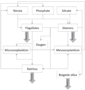
The NORWegian ECOlogical Model (NORWECOM;Aksnes et al., 1995; Skogen and Søiland, 1998) is coupled online to the physical HYCOM model. It uses the HYCOM facility for advection of tracers and they both have the same time-step. NORWECOM has been used in several studies of the North Atlantic and the Norwegian Sea (Hansen and Samuelsen, 2009; Hansen et al., 2010; Skogen et al., 2007). We refer toSamuelsen et al. (2015)for more details about the model and its coupling with HYCOM. The current version includes two classes of phytoplankton (diatoms and ﬂagellates), two classes of zooplankton (meso- and microzooplankton) derived with the same zooplankton feeding parameterization from the model ECOHAM4 (Pätsch et al., 2009), three types of nutrients (inorganic nitrogen, phosphorus and silicon) and detritus (nitrogen, phosphorus), biogenic silica, and oxygen; so that the ecosystem state vector is made of 11 variables. The interactions between the different components of the model are depicted inFig. 2.

The chlorophyll-a concentration (CHLA) is computed from the model diatom and ﬂagellate concentrations (DIA and FLA) through Eq.(1).

CHLA ¼DIA þ FLA

11 ð1Þ

The constant conversion factor 11 mg N/mg Chla is used to obtain the chlorophyll concentration in mg/m3_{, the standard unit of data}

(4)

The physical component of the model was initialized in 1973 from climatology followingSakov et al. (2012). Then, the coupled ocean-ice model was run until the end of 1999. The ecosystem component of the model was activated on 1 January 2000. The initialization of NORWECOM was done using climatological values of nutrients and

oxygen while all other variables were set to a constant low value. Finally, the fully coupled ocean-ice-ecosystem model was run until 1 September 2006, the date of the ensemble generation (see §2.3for more details). Nutrients and oxygen concentrations are relaxed to cli-matology at the lateral boundaries. The model includes an additional barotropic water flux of 0.8 Sv through the Bering Strait, representing the inflow of Pacific water. This inflow is balanced by an outflow at the southern boundary of the domain in the Atlantic Ocean. At the surface, the model is forced with 6-hourly atmospheric fluxes from ERA Interim forcing (Dee, 2011). The river forcings are generated using a hydrological model – (TRIP;Oki and Sud, 1998). The river outflow calculated by TRIP is combined with data from Global Nutrient Export from Watersheds (GlobalNEWS;Beusen et al., 2009; Seitzinger et al., 2005, 2010) and used as nutrient river input to the model. Sea surface salinity is relaxed back to the climatology with a relaxation timescale of 200 days, while no relaxation is applied to the sea surface temperature.

2.2. Assimilated observations

Despite previous studies (e.g.Berline et al., 2007; Ford et al., 2012) reporting potential negative impacts of data assimilation in the physical component of the coupled model on the distribution of nutrients (typically nitrate), improvements are still expected in the Arctic Ocean due to a more realistic positioning of the ice-edge, which control the position of ice-edge blooms (Engelsen et al., 2002).Samuelsen et al. (2009)with an older version of the TOPAZ system, showed that the largest impact of assimilating physical data on the ecosystem compo-nent was near the ice edge. However, the study could not conclude on the quality of the ecosystem state variables due to a lack of independent data for validation. We therefore expect a positive effect of assimilating

120 o W 60o_W 0 o 60 oE 120o E 180 oW 18 o N 36 o N 54 oN 72 oN Boreal Polar Province Atlantic Arctic Province Atlantic Subarctic Province N. Atlantic Drift Province Gulf Stream Province N. Atlantic Subtropical Gyral Province (West)

N. Atlantic Subtropical Gyral Province (East)

N. Atlantic Tropical Gyral Province (TRPG)

Station M

Fig. 1. Spatial domain and some Longhurst-based provinces of interest for the parameter estimation. Station M (66° N, 2° W) is highlighted by a red cross.

(5)

both physical and ocean color observations in the vicinity of sea ice and possibly a degradation of nutrients.

The observations consist of GlobColour 8-day averaged chlorophyll-a mchlorophyll-aps (CHLA), chlorophyll-along-trchlorophyll-ack Sechlorophyll-a Level Anomchlorophyll-alies (SLA) from schlorophyll-atellite altimeters, Sea Surface Temperature (SST) from NOAA, and ice concen-trations (ICEC) from OSI-SAF. The system uses weekly assimilation cycles, and assimilates the gridded SST and ICEC for the day of the anal-ysis, the gridded CHLA for the 8-day window including the day of the analysis and along-track SLA for the week prior to the day of the analy-sis. It results in an overlapping of the 8-day windows of the CHLA obser-vations which means that during the year some obserobser-vations are assimilated twice.

The ocean color data used for assimilation are the GlobColour2 GSM-derived CHL1 products obtained from MERIS, MODIS and SeaWiFS instruments. They correspond to an 8-day averaged chlorophyll-a con-centration for case I water at 25 km resolution. Their spatial coverage varies strongly with seasons resulting in absence of observations for the Arctic Ocean in winter. Chlorophyll-a concentrations are assumed to be log-normally distributed (Campbell, 1995) and the observations are thus log-transformed before assimilation. The standard deviation of these log-transformed observations is assumed equal to 0.35, so the observation error equals 35% of the observation values (Gregg and Casey, 2004). Locally the true errors can be larger than 35%, resulting in a large underestimation of the observation error that can impair the quality of the estimated variables. This is the case in the Arctic Ocean in 2010 for which erroneously high concentrations occur due to a deg-radation in the quality of the MODIS Aqua ocean color product for this version of the GlobColour data set (Meister and Franz, 2014). Further-more, the algorithm used for deriving chlorophyll estimates in case I water is unsuited to coastal waters. In compensation, observations in waters shallower than 300 m and less than 50 km away from the coast are not assimilated in the first 6 months of 2008 in order to pre-vent overfitting to observations of poor quality. However, such criterion exclude large areas of interest (e.g. North Sea, Chukchi Sea, Hudson Bay) that would benefit from assimilating case I water chlorophyll concen-trations. So, all the observations located at least 50 km away from the coast are assimilated from 1 July 2008. It means that the estimation of the ecosystem parameters starts in these areas with a 6-month delay compared to other North Atlantic open ocean areas (this delay is shorter at high latitudes because there are no observations during winter time). Except for the SST product, the physical observations correspond to the ones assimilated in TOPAZ4 (Sakov et al., 2012). The use of version 2 of the Reynolds SST product (Reynolds and Smith, 1994) from the National Climatic Data Center3 _{(NCDC), with a resolution of approximately} 100 km, is motivated by the coarse resolution of the model. We refer to

Sakov et al. (2012)for more details regarding the observations of SLA and ice concentration as well as the calibration of their error variances.

For all types of observations, a preprocessing step is performed and includes a range check and a horizontal superobing (averaging of the observations present in the same model grid point).

2.3. Data assimilation system

The data assimilation system is derived from the TOPAZ4 system (Sakov et al., 2012) and uses a deterministic scheme of the EnKF (DEnKF,Sakov and Oke, 2008). The choice of this ﬁlter is motivated by the overestimation of the posterior error variance, which is an apprecia-ble property when estimating parameters as it prevents the spread of the parameter ensemble from being reduced too quickly. Indeed, better performances of the DEnKF compared to the stochastic EnKF (Burgers et al., 1998; Evensen, 2003) have been reported bySimon and Bertino (2012)in their experiments of combined state parameter estimation in a simple NPZ model.

The analysis is performed in the model grid space on a weekly basis. The weekly cycles follow the availability of the physical observations, and the date of the analysis is used to define which 8-day averaged chlo-rophyll data set is assimilated. The analysis is divided into two steps. In a first step, the physical data (SST, TSLA and ice concentration) are assim-ilated in the physical component (HYCOM) of the coupled model, and the biological component is not included in the analysis state vector. The instances of negative layer thickness or ice concentration, should they occur, are corrected in a post-processing procedure. The biological variables are tracer concentrations, so that any update of the layer thick-ness during the assimilation of physical data does also change the tracer mass in the layer. In order to ensure the conservation of the amount of species for each tracer at each horizontal grid point (conservation in the water column), a vertical remapping of the tracer is also performed. This remapping uses the WENO polynomial interpolations (Jiang and Shu, 1996) that are already embedded in HYCOM. This approach can re-sult in a large local increase (resp. decrease) of the tracer concentrations in cells affected by a strong reduction (resp. increase) of their volume before assimilating ocean color observations as highlighted in §3.2. However, it has no impact on the innovations – the differences between the modeled and observed surface chlorophyll-a concentrations – in the second step due to the choice of the hybrid coordinate system. Because the top 5 layers are z-layers, the volume of their cells does not change in the physical analysis step and the surface chlorophyll-a concentrations are the same before and after assimilating physical data. It results in eco-system analysis steps that compute the innovations using the forecast concentrations. As suggested more recently byJanjić et al. (2014), the introduction of the constraint of mass conservation in the estimation process could be a more elegant solution for remedying the issue of mass conservation with ensemble-based Kalman filter (if practically tractable).

In the second step, surface chlorophyll concentration data are assim-ilated in the biological component (NORWECOM) of the coupled model. The dynamics of the physical ocean is thus not corrected via assimilation of biological data. The estimation of four parameters – the mortality rates of two groups of phytoplankton and zooplankton – is done by aug-menting the biogeochemical state vector with these parameters. The latter state vector is thus made of eleven 3D state variables and four 2D parameters. These parameters have been chosen due to the large uncertainties they introduce in the closure of the ecosystem model. Biological state variables and parameters are log-transformed prior to assimilation in order to prevent issues arising from the positiveness of the variables. The choice of the logarithmic function rather than empir-ical anamorphosis functions was motivated by the constraints resulting from the near operational framework of the study: the robustness of the transformation when applied to bounded parameters (the potential discontinuities of the distribution at the bounds are not handled by the piecewise linear anamorphosis function and require an extrapolation of the distribution near the bounds) and the promising results obtained in a previous simpler application (Simon and Bertino, 2012).

The assimilation uses a distance-based localization method known as local analysis (Evensen, 2003; Sakov and Bertino, 2011). A local analysis is computed for one horizontal grid point at a time, using obser-vations from a spatial window around it. A smoothing procedure is part of the local analysis, and it consists of multiplying local ensemble anom-alies by a quasi-Gaussian, isotropic, distance-dependent localization function (Gaspari and Cohn, 1999). The localization radius is constant and is set to 300 km for the assimilation of physical data following

Sakov et al. (2012)and 200 km for the assimilation of ocean color data. The localization radius for physical assimilation is higher in order to avoid the generation of gravity waves. Furthermore, a lower localiza-tion radius in the assimilalocaliza-tion of ocean color is coherent with the greater differences between local ecosystem in coastal and open seas. Finally, the use of an ensemble of small size compared to the dimension of the problem leads to an underestimation of the error variances (Houtekamer and Mitchell, 1998). A solution for this issue consists of

2 _{http://www.globcolour.info}_. 3 _{www.ncdc.noaa.gov}_.

(6)

multiplying the empirical covariance matrix (or anomalies) by a scaling factor called inﬂation (Anderson and Anderson, 1999; Hamill et al., 2001). Inﬂation is introduced both for the state variables and parameters for which observations are only assimilated locally: the values are 1.01 for both the physical and biogeochemical state variables and 1.06 for the NORWECOM parameters.

Random perturbations are introduced to the atmospheric forcing in order to emulate uncertainties in the surface forcing. The random per-turbations are generated by a spectral method (Evensen, 2003) using a spatial decorrelation radius of 250 km. The decorrelation time-scale is two days. The standard deviations of the perturbed ﬁelds follow those proposed bySakov et al. (2012). These perturbations induce small differences within members of the ensemble, in particular in the mixed layer depths, the mixed layer temperature and position of the ice edge. The perturbations induced in the physical dynamics then cascade into the ecosystem component of the coupled model. However, biological parameters are not perturbed during the forecast steps and remain constant between two analyses (justifying the larger inﬂation factors for the parameters).

The initial ensemble is generated on 1 September 2006 so that it contains explicit variability both in the interior of the ocean and at the surface. It consists of the model snapshot taken from the free run model simulation described in §2.1. Using this snapshot, 100 initial states are produced by perturbing the layer and ice thickness by 10% with a decorrelation length scale of 50 km. The perturbation of layer thickness also has a vertical decorrelation distance of three layers. The parameter ensemble is initialized by assuming that the parameters are log-normally distributed around their nominal values (5% per day for both phytoplankton mortality rates and 20% per day for both zooplank-ton mortality rates) with a 50% error. The initial ensemble is then inte-grated for three months to damp dynamical instabilities that result from the perturbations. After generating the initial ensemble, the data assim-ilation system was spun up with only assimassim-ilation of physical variables during a period of one year, for the calendar year of 2007. During that time, the ecosystem model was kept in free run mode. The assimilation of chlorophyll concentration data starts gradually on 1st January 2008. At that date, the spread of the ensemble could be very large compared to the observation error due to the use of perturbed parameters and atmospheric forcing that enhanced the error growth during one year. In order to prevent an initial shock of the ecosystem due to strong corrections (that could result in a filter divergence and/or an overfitting to the observations), the observation error is multiplied by a factor 8 during the first month (January). Then, this factor is divided by two every month and reaches the value one in April 2008. This approach has an impact on the state and parameter estimation because it artifi-cially decreases the amplitude of the corrections during this 3-month initialization period. For that reason, the discussion of the results in §3.1

does not take into account the values estimated during this period despite signiﬁcant corrections (see for instanceFig. 3and the zooplankton mortality rates on 5 March 2008).

Finally, due to the large computational costs and long time required for running the system over long periods, some modiﬁcations and ﬁxes have been applied to the system during the experiments instead of parallel experiments. These changes are summarized inAppendix A.

2.4. Validation

The validation is done by comparing the outputs of ecosystem com-ponent of the data assimilation system to different observations. These include the assimilated 8-day average chlorophyll concentration, inde-pendent in-situ data at station M (66° N, 2° W) including time series of chlorophyll, nitrate, silicate and phosphate concentrations. The latter come from the MyOcean INS-TAC (Arctic) sources and have been gathered and quality checked by the Norwegian Institute of Marine Research (IMR).

We also performed a simulation without any data assimilation. Thus, the model was deterministically run from 1 September 2006 – from the output ﬁle used in the generation of the ensemble – to 31 December 2010. This simulation is referred to as the “free run” in the rest of the manuscript, and is used to assess the added value of data assimilation. 3. Results

3.1. Parameter estimation

The EnKF estimates the spatially varying biological parameters of the NORWECOM model from January 2008 to December 2009. Due to local collapses of the parameter ensemble in a few dynamical areas in late 2008, new values of the parameters have been drawn on 1 January 2009. This was done to increase the spread of the ensemble in these areas (while preserving the mean) in order to further correct the parameters in 2009. More details about this draw can be found in

Appendix A. At the end of 2009, the parameter values were frozen and no longer updated for the rest of the experiment. At each grid point, an averaging (both in space and time) of the values obtained after the analysis during the period April 2008–March 2009 is performed to pro-duce a set of weekly optimized parameter maps. This 3-month shift in the parameters' yearly cycle is motivated both by the exclusion of values obtained during the warm-up of the assimilation of chlorophyll-a obser-vations (artificial increase in the observation error from January to March 2008) and by the exclusion of constant values associated with local filter divergences that occur again during spring 2009. These maps are then used in 2010 to assess the performance of the data assimilation system in a pure state estimation configuration.

3.1.1. Regional distribution of the estimated parameters

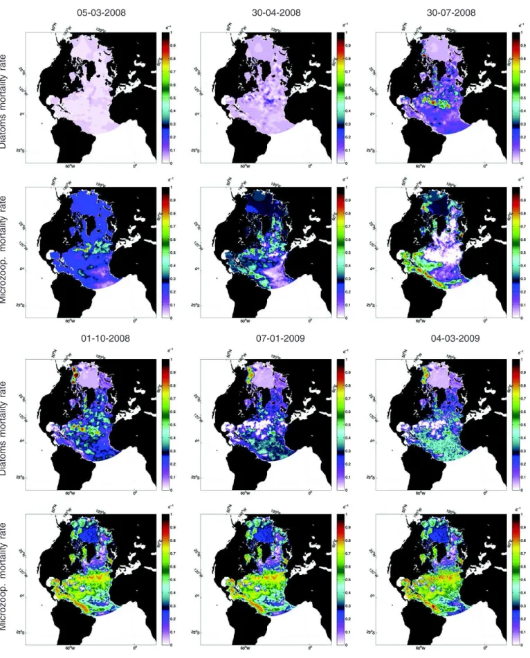
We are interested in the spatio-temporal evolution of the estimated parameters.Fig. 3shows the spatial distribution of both the diatom and microzooplankton mortality rates after the analysis step on several dates in 2008 and 2009. First, we note that the data assimilation leads to strong corrections of both parameters compared to their prior values. Thus, mortality rates larger than 70% per day or lower than 0.001% per day occur locally while their prior values are equal to 5% or 20% depend-ing on the plankton type (phyto- or zoo-). However, these changes in the parameters can be locally non-monotonic and seasonal variations are observed in some local regions (e.g. North Atlantic Subtropical Gyral Provinces, Gulf Stream Province). This result strengthens the con-clusions of recent works (Mattern et al., 2012; Roy et al., 2012) suggest-ing the use of time-dependent parameters in biological ocean models.

Secondly, regional patterns clearly emerge from the series of maps for both parameters. The differences in the regional evolution of the pa-rameters seem to coincide with some of the biogeochemical provinces deﬁned byLonghurst (1995). In order to analyze locally the distribution of the parameters, we deﬁne a partition of the North Atlantic and Arctic Oceans based onLonghurst (1995). These regions are highlighted in

Fig. 1.

On the one hand, the parameters tend to converge towards constant values in coastal regions like the Guiana Coastal Current, the Chukchi, Beaufort and Barents Seas in the Arctic Ocean, the Baffin Bay, the Cana-dian Archipelago, the Hudson Bay and the North Sea. The extreme values that are reached may either be associated with a bias in the model (e.g. erroneous nutrient inflow from the Pacific Ocean through the Bering Strait), with erroneously large values in the observation due to large concentrations of particles associated with river discharges (e.g. from the Amazon), or with local differences in the ecosystem due to the presence of sea ice for instance (e.g. Baffin Bay). However, the lack of ocean color observations in the Arctic Ocean in fall and winter implies that no corrections to the parameters can be made during those seasons, which prevents their seasonal variations.

On the other hand, strong seasonal variations in the parameters are observed in open-ocean areas like the North Atlantic Subtropical Gyral

(7)

Provinces (both East and West: STPE, STPW), the Eastern part of the North Atlantic Tropical Gyral Province (TRPG), the Gulf Stream Province (GUSP) and the North Atlantic Drift Province (DRIP). Weaker seasonal

variations are seen in the Atlantic Arctic (ARCP) and Sub-Arctic (SARP) Provinces. We refer to §3.1.2for more details about the time evolution of the optimized parameters in the GUSP, DRIP, ARCP and

30-07-2008

30-04-2008

05-03-2008

04-03-2009

07-01-2009

01-10-2008

Diatoms

m

ortalit

y

rate

Microzo

op.

mortalit

y

rate

Diatoms

m

ortalit

y

rate

Microzo

op.

mortalit

y

rate

(8)

SARP provinces. We note that the simulated chlorophyll concentrations tend to be too low during the cold periods and too large during the spring blooms when constant parameter values are used (not shown). NORWECOM has been developed and tuned primarily for high-latitude regions and thus represents the plankton community in the Arctic Ocean and the Norwegian Seas better than other areas. In these areas, the seasonal variations of the parameters could be explained by a better modeling of the time-dependence of the ecosystem which is not properly taken into account with constant parameters. However, the corrections on the parameters at middle latitudes and in the tropical regions do not highlight a specific time-dependence of the ecosystems, but rather compensate for large model errors. For instance, two specific important components in the tropics can be mentioned: the abundance of nitrogen fixing bacteria and the importance of the microbial loop and regenerated production. Neither of these processes are explicitly repre-sented in this model, although remineralization of nutrients is parame-terized in a simple way. Nevertheless, this result suggests that the use of time-dependent parameters is needed to better represent the local dynamics of the ecosystems either for dynamically improving the parameterizations or compensating for model errors associated with unresolved processes.

Finally, we note a pattern of extreme low values of the diatom mor-tality rate in the STPE province and the GUSP province that does not evolve in 2009. In that area, a ﬁlter divergence occurs at the end of 2008 for the diatom mortality rate component of the ensemble. The strategy that we adopted to remedy this issue – a redraw of the param-eters early 2009 based on the last value reached on 31 December 2008 and an assumption of lognormal distribution – is insufﬁcient to recover realistic parameters values. These locally low diatom mortality rate values are responsible for the strong bloom during spring 2009 (see §

3.2.1). It results in a large increase of the error that cannot be corrected by the assimilation due to the low spread of the diatom mortality rate (weak corrections of the parameter). Further strategies for restarting the parameter estimation after ﬁlter divergence should be investigated. 3.1.2. An example of local evolution of the optimized parameters used in 2010

We consider the following question: What is the value of re-using parameters estimated in a year during the next year? In analogy with a steady-state Kalman Filter, this approach could save signiﬁcant com-puter power. Thus, we are interested in the local evolution of the weekly maps built from the optimized parameters and used in 2010 (i.e., no pa-rameter estimation). Within each Longhurst-based province deﬁned in

Fig. 1, we computed the spatial mean value and standard deviation of the four parameters and focused on their yearly evolution. We recall that these weekly maps (52 in total) have been produced from the daily average outputs of the model during the period April 2008– March 2009 by averaging the values of the parameters both in space and time. The temporal averaging is done over an 11-week window centered on a targeted week with the weights [1 2 … 6 … 2 1] assuming periodicity in time (the values in January 2009 are assumed to be repre-sentative of the values in January 2008). Depending on the area, this as-sumption cannot be fulﬁlled by the parameters resulting in strong discontinuities in their values between the end of March and the begin-ning of April. For instance, the values of the ﬂagellate mortality rate in late March 2009 are 10 times larger than the values obtained in early April 2008 in the Gulf Stream Province. In all of these cases, the applica-tion of the temporal averaging smoothes the strong discontinuities in the parameters' time series, and further prevents a shock of the ecosys-tem in early spring of the 2010 run. The spatial averaging is done by applying a full weighting restriction operator (for more details, see

Trottenberg et al. (2001)) followed by a linear interpolation, both with a resolution ratio equal to 3. This procedure ﬁlters out the high frequen-cies (small scales) that lie in the null space of the restriction operator.

Figs. 4 and 5represent the temporal evolution of the spatial mean values and standard deviations of all parameters in the Gulf Stream

Province (GUSP), the North Atlantic Drift Province (DRIP), the Atlantic Arctic Province (ARPC) and the Atlantic Sub-Arctic Province (SARP). In these provinces, the assimilation of data led either to seasonal variations in the parameters, or to convergence towards larger values during the estimation process (Fig. 3). First, we note that the parameters are corrected rather severely, with the exception of the mesozooplankton mortality rate in the ARCP and SARP provinces. However, their strong decrease during the period from late February to early May (marked by dashed lines) should not be considered meaningful for most of the parameters. During this period, values from March 2009 and April 2008 are used to build the time series of weekly optimized parameters. Strong variations of the parameters highlight discontinuities in the time series, and the limits of our assumption of periodicity.

With the exception of this period, we note first that the dynamics of the flagellate loss rates differ from the others in most provinces. Indeed, the flagellate loss rate tends to converge towards large values in the GUSP, ARCP and SARP provinces, and most likely in the DRIP province as well, while the diatoms, micro- and mesozooplankton loss rates ex-hibit seasonal variations in most of the provinces.Fig. 6shows the tem-poral evolution of surface diatoms, flagellates and chlorophyll-a concentrations in these four provinces from April 2008 to March 2009. The jigsaw is typical of the Kalman filter corrections done in the succes-sive analysis steps. The strong decreases in both phytoplankton concen-trations confirm that the model is too productive during the spring bloom. Furthermore, the analysis steps tend to reduce the flagellate con-centrations from April to May 2008 until fall 2008. This is in agreement with the large increase in the flagellate loss rate that starts in spring and the stabilization around large values that follows in summer/fall. In the same way, the large corrections leading to a decrease in the diatom con-centrations during the spring bloom, can be associated with the large in-crease in the diatom loss rate. Furthermore, the small inin-crease in the diatom concentrations in the GUSP province starting early Fall 2008 can be associated with the strong decrease in the diatom loss rate, resulting in seasonal variations in this province. Finally, we note that both zooplankton loss rates exhibit seasonal variations in the four prov-inces. This could either be associated with temporal changes in the biol-ogy or else betrays a model bias (too strong production during spring and too low production in winter) and/or assimilation biases as well. 3.1.3. Definition of regional provinces based on a clustering analysis of the estimated parameters

Estimating spatially distributed parameters in near operational data assimilation systems can result in an increase of the dimension of the problem, and thus the computational cost. A solution for reducing the dimension of the problem consists of defining provinces to which one associates spatially constant parameters. A priori strategies can be based on uniform partitions of the spatial domain (Losa et al., 2004), the use of the Longhurst provinces (Doron et al., 2013), or geophysical considerations – for instance the distinction between estuaries, coastal water and open oceans (Mattern et al., 2012). However, estimating pa-rameters over long periods, as we did, leads to the production of a large data set that can be helpful for defining a posteriori clusters that could define the parameter grid for future parameter estimation experiments. So, our aim is to explore the ability to exploit the data produced by the parameter estimation (e.g. the weekly maps of optimized parameters), in order to define consistent provinces using the information provided by both the model and the observations.

As both geographical and biological information have to be consid-ered, the clustering is processed in two steps. First, a K-means method (MacQueen, 1967) is applied to the optimized parameters to generate a partition of the estimated parameters in the North Atlantic and Arctic Oceans. The procedure follows a simple and easy way to classify a given set of parameters into an – a priori fixed – number of clusters. The main idea is to define k centroids – one for each cluster which represents the mean of the estimated parameters assigned in the same cluster. The number of clusters k is defined so as to minimize the within-cluster

(9)

sum of squares. Second, because the estimated parameter clusters could gather different geographical regions that do not intersect, the contours of each estimated parameter cluster are extracted. As the clusters could have arbitrary shapes, spectral clustering (Ng et al., 2002) is applied to de-fine geometrically separated clusters. It selects the dominant eigenvectors of a parameterized Gaussian affinity matrix in order to build a low-dimensional data space wherein the geometrical data are grouped into clusters (Mouysset et al., 2014). The final clustering result is a partition of the oceans into geographical patches that have distinct parameter sets.

Fig. 7shows the 13 provinces obtained from our clustering analysis over the whole domain including coastal areas and the 7 provinces in open waters that we derived from the Longhurst provinces (Fig. 1). Each color and number highlights a regional province, except for the cyan color (province 1) that corresponds to areas for which few or no corrections were applied to the parameters during the assimilation due to lack of observations (area under the ice in the Arctic Ocean and some coastal areas).

First we note that the clustering analysis leads to regional provinces that are consistent with the Longhurst provinces in the northern part of the domain. Even if they do not exactly match, most of the Longhurst-based provinces clearly emerge from the clustering analysis. Thus, clus-ters can be associated with the Gulf Stream Province (cluster 10), the North Atlantic Drift Province (cluster 8), the North Atlantic Subtropical Gyral Province (both West and East, clusters 11 and 12) and the Atlantic Arctic Province (cluster 5). The analysis of the local evolution of the pa-rameters allows the detection of differences in the plankton dynamics due to the ice coverage – see for instance the two different clusters highlighting the seasonally ice covered Bafﬁn Bay (cluster 4) and the open Labrador Sea (cluster 5) – or between the two sides of the Gulf Stream (clusters 9 and 10). Other coastal Longhurst provinces (not shown inFig. 1) like the North Sea (cluster 7) are also highlighted by the clustering analysis.

However, important differences arise as well. First, the Boreal Province is now divided into four clusters: the Beaufort Sea (cluster 2), the Hudson Bay (cluster 3), the Baffin Bay (cluster 4) and the part of the Boreal Province for which few or almost no observations were as-similated (cluster 1). These differences (for instance erroneous nutrient input specified at the Bering Strait and the Hudson River) can be attrib-uted to various sources of model errors, but they can also suggest that the Arctic Ocean presents various ecosystems and so, a refinement of the Boreal Province should be considered. For instance, the annual mean values of the parameters (not shown) suggest that the cluster highlighting the Beaufort Sea is mostly characterized by a large increase in the diatom loss rate and almost no changes in the flagellate loss rate, while the cluster highlighting the Baffin Bay is characterized by an in-crease in the loss rate of both zooplankton groups, as is the Hudson Bay cluster. Similarly, we note the occurrence of a small cluster (6) associated with the Seas west of Scotland, suggesting that the Northeast Atlantic Continental Shelf province could be divided into two sub-provinces when estimating parameters: the North Sea and the seas west of Scotland. Further work based on the analysis of in-situ data should be done to determine if the different clusters highlight biological dynamics specific to these areas. However, this is out of the scope of the present study. Another aspect that needs further investigation is the dynamic definition of the provinces in the Arctic Ocean. For instance, the spatial domain of the provinces could evolve in time accordingly to the evolu-tion of the ice extent. This would better take into account current changes in the ice coverage in the Arctic Ocean.

Moving southward, we note that the analysis of the parameters does not highlight differences between the Atlantic Arctic Province and the At-lantic Sub-Arctic Province. Both provinces are merged into cluster (5) that extends from the Labrador Sea to Svalbard. The Barents Sea does not belong to this province and is rather associated with the Boreal Arctic Province. This is probably due to the small amount of observations that Fig. 4. Optimized parameters: The temporal evolution of the four loss terms in the Gulf Stream Province (GUSP) and the Atlantic Drift Province (DRIP). The dark gray line shows the base value for the parameter. The transparent areas highlight the period for which values from 2008 to 2009 were simultaneously used to build the optimized set of parameters (temporal averaging assuming one-year periodicity).

(10)

have been assimilated in that area, or else the coarse model resolution. Fi-nally, the clustering analysis leads to a big province (cluster 13) covering the Gulf of Mexico, the Caribbean, the Guyana Current Coastal and the Eastern part of the North Atlantic Tropical Gyral Province. In this province, the parameters tend to converge towards extreme values (either low or high) possibly due to model errors. As stated earlier, the model targets high latitude ecosystem dynamics and does not explicitly represent im-portant processes in the Tropics. Again due to a large model error, we note a large cluster (12) covering the western part of the North Atlantic Tropical Gyral Province, connecting the North Atlantic Subtropical Gyral Province (East), for which the parameters tend to exhibit strong seasonal variations. Thus, clustering analysis leads to a split of the Longhurst-based North Atlantic Tropical Gyral Province into two large West and East prov-inces based on the differences in the spatio-temporal evolution of the pa-rameters. Thus, the results show that model error should be considered when deﬁning a priori spatial partition of the model parameters. 3.2. State estimation

We are now interested in the quality of the estimation of the ecosys-tem state variables. The output of the data assimilation solution is compared to both assimilated and independent in-situ observations. 3.2.1. Validation against assimilated observations

The assessment of the quality of the estimation is done by comput-ing the time evolution of the root mean square error (RMS) and stan-dard deviation of the ensemble (STD):

RMS tð Þ ¼n ffiffiffiffiffiffiffiffiffiffiffiffiffiffiffiffiffiffiffiffiffiffiffiffiffiffiffiffiffiffiffiffiffiffiffiffiffiffiffiffiffiffiffiffiffiffiffiffiffiffiffiffiffiffiffiffiffiffiffiffiffiffiffiffiffiffiffiffiffiffiffi 1 #Ω X k∈Ω y tðn;kÞ−H xð Þ tðn;kÞ # $2 r STD tð Þ ¼n ffiffiffiffiffiffiffiffiffiffiffiffiffiffiffiffiffiffiffiffiffiffiffiffiffiffiffiffiffiffiffiffiffiffiffiffiffiffiffiffiffiffiffiffiffiffiffiffiffiffiffiffiffiffiffiffiffiffiffiffiffiffiffiffiffiffiffiffiffiffiffiffiffiffiffiffiffiffiffiffiffiffiffiffiffiffiffiffiffiffiffiffi 1 N−1 1 #Ω X k∈Ω XN m¼1 x m _t n;k ð Þ−x tðn;kÞ ð Þ2 r ð2Þ

with Ω is the domain of computation, # Ω is the number of grid points of the domain, N is the number of members, y denotes the observations (e.g. chlorophyll concentration), HðxÞ corresponds to the ensemble mean of the observed variables (e.g. chlorophyll concentration), and x refers to the ensemble mean.

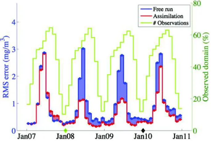
The domain-averaged RMS error and STD time series are shown in

Fig. 8. These quantities are computed at the date of the analysis from re-start files of the model and the assimilated observations. Two values of RMS error and STD are calculated on each date: the first uses the fore-cast ensemble (before the analysis step) and the second is based on the analysis ensemble. This explains the high frequency peaks that we observe inFig. 8reflecting the decrease of the errors due to the analysis step. To illustrate, we first note a seasonal peak of errors during the sum-mer phytoplankton bloom. The first peak corresponds to the physical data assimilation-only in 2007 and the following peaks refer to the as-similation of chlorophyll concentration data from 2008 to 2010 with the characteristic see-saw evolution. It is worth noting that the assimi-lation of chlorophyll concentration data has proven effective in the first year (2008): even in a 7-day window, the forecast errors remain well below the errors obtained when assimilating the physical data only or those obtained from a free-run simulation (no data assimila-tion). The errors predicted by the EnKF (blue line) correlate well with the variations of the actual errors, but underestimate the errors by half in the main bloom period (from May to August), indicating that the model and measurement errors are well tuned for late summer and winter conditions, but that additional sources of errors could be consid-ered for the summer (e.g. the optical properties of the water).

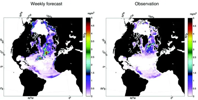
One can also notice a large growth of the RMS errors during the bloom period in 2009. This is mostly due to the erroneous large concen-trations located in a few restricted areas of the domain (e.g. the STPW province around 30°N), as shown inFig. 9. In these areas, the parameter estimation leads to a combination of values that encourages the Fig. 5. Optimized parameters: The temporal evolution of the four loss terms in the Atlantic Arctic Province (ARPC) and the Atlantic Sub-Arctic Province (SARP). The dark gray line shows the base value for the parameter. The transparent areas highlight the period for which values from 2008 to 2009 were simultaneously used to build the optimized set of parameters (temporal averaging assuming one-year periodicity).

(11)

phytoplankton growth – low phytoplankton and large zooplankton mortality rates (seeFig. 3) – due to too-low chlorophyll concentrations in winter 2008–2009. However, the spread of the ensemble is locally too small in early spring and hence, it does not allow for large corrections of parameter values that would be required during the spring bloom in 2009 (too-large chlorophyll concentration). This local ﬁlter divergence does not occur in the Arctic Ocean (the targeted area of the MyOcean pilot reanalysis) in 2009 and we note that the assimilation of ocean color data results in a large reduction of the RMS error in this area also in 2009. The reader may refer toAppendix Bfor more details on the evaluation of the surface chlorophyll in the MyOcean pilot reanalysis product.

In the year 2010, the parameters are assumed equal to the weekly averaged values estimated from April 2008 to March 2009. After two years of parameter estimation, the spread of the ensemble appears to be too small in some local areas and not allowing for large corrections anymore. The use of optimized time varying parameters is expected to lead to better results compared to the ones we could have obtained with parameters resulting from a locally-diverged ﬁlter. Yet, the RMS errors seem to increase back to the high levels obtained with the free run or before assimilating chlorophyll concentration data. This could be related to the poor quality of the data assimilated during that year as mentioned in §2.2. So, sparse erroneous large values occur in the Arc-tic with a spatial distribution that changes every week. This leads to an underestimation of the observation error in the ﬁlter and results in erro-neous large increase in the chlorophyll concentration in the vicinity of these observations, and large increase in the RMS error at the next cycle due to changes in the position of these artifacts. This issue stresses the need for reliable uncertainty estimates on operational satellite prod-ucts. Furthermore, the increase in the RMS error in 2010 could also be

related to the inability of the model to simulate the unusually strong negative North Atlantic Oscillation (NAO) that occurred in 2010 and was responsible for a “highly anomalous phytoplankton bloom” (Henson et al., 2013). This also highlights the fact that estimating biological model parameters is a critical aspect of data assimilation in biological models.

3.2.2. Validation against independent in-situ observations

Data assimilation results are compared to in-situ data for chlorophyll and nutrients available at station M (66° N, 2° W) in the Norwegian Sea. The model values used were those of the grid cell and layer containing the measurement – no interpolation was done. The model daily aver-ages were compared to the in-situ data, and if there were more than one measurement at any grid-cell during one day, we used instead the mean of these measurements. The observations of station M are the only time-series measurements available for the reanalysis period, but unfortunately data for the last year (2010) are not available yet. Further-more, data can be missing in December and/or January depending on the year, resulting in an incomplete time-series for the period 2007– 2009.

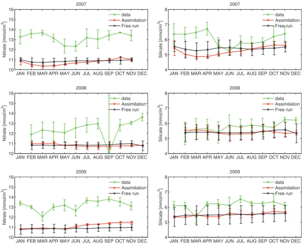
Figs. 10 and 11show the monthly time series of mean value and standard deviation of surface chlorophyll, nitrate, phosphate and silicate concentrations from 2007 to 2009. First we note that assimilating only physical data in 2007 leads to an improved surface chlorophyll concen-tration compared to the free-run simulation during the entire year, despite a larger overestimation of the chlorophyll concentration in April and May. This improvement may be due to a more realistic repre-sentation of the mixed layer. Indeed, the assimilation improved the model representation of surface temperature and surface salinity (not shown) when compared to in-situ measurements (only available for Fig. 6. Model daily averages: temporal evolution of the spatial mean surface diatoms (black), ﬂagellates (red) and chlorophyll-a (green) concentrations plus/minus a standard deviation in the Gulf Stream Province (GUSP), the Atlantic Drift Province (DRIFT), the Atlantic Arctic Province (ARPC) and the Atlantic Sub-Arctic Province (SARP) from April 2008 to March 2009.

(12)

2007 and 2008). The assimilation of surface chlorophyll concentrations in 2008 and 2009 results in a signiﬁcant reduction of the bias in the data assimilation as compared to the free run. The mean chlorophyll concen-trations are weaker during the bloom and the standard deviations are closer to the observed ones for most of the months.

One particular point of interest for the in-situ comparison is the effect of chlorophyll assimilation on the concentrations of nutrients. From the surface nutrients, we see that the data assimilation simulation tends to be slower in mixing the nutrients back to the surface during the winter, otherwise the two runs are fairly similar. The difference in winter concentration can be observed also in 2007 (when biological assimilation is not performed) and is probably a result of assimilating

physical variables. During the spring bloom in March and April, primar-ily dominated by diatoms, we see a change of the silicate concentration between the free run and assimilation runs. Nevertheless, during the summer period silicate concentrations are the same (depleted to near 0) in both runs while the observations show that not all of the silicate is depleted. We also note that the nitrate and phosphate concentrations from the assimilation run are higher at the surface from those of the free run during the summer of 2009. This is an effect of the ﬂagellate bloom that has been suppressed by the assimilation during summer, resulting in surface nitrate and phosphate concentrations that are in better agreement with the observations in late 2009 compared to the free run simulation.

Fig. 8. Surface chlorophyll concentration: time evolution of the RMS error and standard deviation computed from the assimilated observation at the date of the analysis (both forecast and analysis). The green diamond highlights the date of the ﬁrst biological analysis. Chlorophyll observation in area shallower than 300 m are introduced in July 2008 (black diamond). No parameter estimation in 2010 (magenta diamond).

120 o W 60o W 0 o 60 oE 120o E 180 oW 18 o N 36 o N 54 oN 72 oN 1 2 3 4 5 6 7 8 9 10 11 12 13

(13)

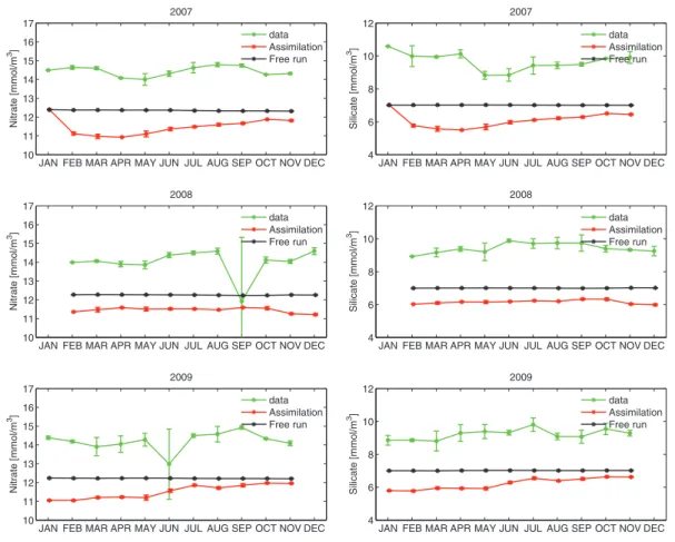
In the depth interval 300–700 m (Fig. 12), the concentrations of sil-icate and nitrate are persistently lower than the observed concentration. There are no large differences between the free run and the assimilation run and we can conclude that the assimilation does not affect the concentration of nutrients very much, however negative effect cannot be detected. On the contrary, in the depth interval 700–1300 m (Fig. 13) we note that the concentrations of nutrients in the assimilation

run are almost always lower than the concentrations of nutrients in the free run except for the last months of 2009. This is a direct consequence of the assimilation shock that occurred at the ﬁrst analysis in January 2007 (when only physical data are assimilated): the large corrections of the layer thickness that occur at depth result in a signiﬁcant decrease of the concentration tracers (around 10%) in the few layers associated with the depth interval 700–1300 m due to the remapping of the tracers Fig. 9. 29 July 2009: surface chlorophyll-a concentration estimated from the mean of the ensemble and satellite observations.

JAN FEB MAR APR MAY JUN JUL AUG SEP OCT NOV DEC 0 2 4 6 8 Chlorophyll [mg/m 3] 2007 data Assimilation Free run

JAN FEB MAR APR MAY JUN JUL AUG SEP OCT NOV DEC 0 5 10 15 Nitrate [mmol/m 3] 2007 data Assimilation Free run

Fig. 10. Station M: monthly mean value and standard deviation of chlorophyll (left) and nitrate (right) concentrations from 2007 to 2009 in the depth interval 0–30 m. In-situ observations are in green, the free run simulation is in black and the data assimilation simulation is in red. Satellite-derived chlorophyll concentrations are assimilated from 2008.

(14)

on the corrected vertical isopycnal mesh. Afterwards, almost 3 years are needed to obtain nutrient concentrations that are close to their initial values. However, the initial shift in the nutrient concentrations in this interval depth (due to the assimilation shock) seems to have little im-pact on the surface processes. We do not observe negative trends or a large shift in the nutrient concentrations in the depth interval 300– 700 m. Nevertheless, the nutrient response at depth is a slow process, hence no deﬁnite conclusion can be drawn until a longer simulation has been produced and a longer in-situ time-series has been obtained and used for validation.

4. Conclusion

We investigated the possibility of estimating both biological param-eters and model state variables with ensemble-based Kalman filters in pre-operational ocean ecosystem models over several years. For that purpose, a combined state-parameter estimation experiment has been conducted in a North Atlantic and Arctic Ocean configuration of the coupled physical-ice-biogeochemical model HYCOM-NORWECOM over the period 2007–2010. Physical and bio-remote sensing data were assimilated every week with the deterministic ensemble Kalman filter. Four biological parameters have been estimated at each grid point during the period 2008–2009, leading to the definition of 2D maps of weekly optimized parameters that were used in the model in 2010. However, the use of the optimized parameters in the last year of simulation (2010) was not found very useful in improving the model performance.

The assimilation of ocean color data led to large deviations of the parameters from their nominal values. Depending on the area, we

note that the parameters tend either to converge towards values that can be extreme (for instance in coastal areas or at Tropical latitudes) or exhibit strong seasonal variations. In areas of the domain where the model is reliable, these variations can be associated with a better model-ing of the time-dependence of the ecosystem, strengthenmodel-ing the recent suggestions to use time-dependent parameters in biological ocean models (Mattern et al., 2012; Roy et al., 2012). On the contrary, in areas where the model is less reliable the variations are associated to large model errors.

The study also suggests that regional patterns emerge from the 2D maps of the parameters during the estimation. In order to identify prov-inces that could be associated with these patterns, we performed a clus-tering analysis of the 2D maps of the optimized parameters. The idea is to identify provinces with which one could associate spatially constant parameters that could be estimated in future experiments, in order to reduce the dimension of the estimation problem. Most of the clusters that we obtained can be associated with the observation-based Longhurst provinces in the northern part of the domain. However, the results of the clustering differ from the Longhurst provinces in the trop-ical area, where the NORWECOM model presents large errors, since it is specifically designed and tuned for high latitudes. This result suggests that the use of a spatial parameter grid defined from observations (e.g. the Longhurst provinces) might not be well adapted for parameter esti-mation in areas with large model error. In our opinion, it is preferable, first to estimate the parameters on a fine resolution partition of the domain – for instance the model grid – over a period long enough to catch seasonal cycles, and then, to define a posteriori provinces from a clustering analysis of the long data set of parameters. This strategy could provide the basis for a – low dimensional – definition of parameter Fig. 11. Station Mike: monthly mean value and standard deviation of phosphate (left) and silicate (right) concentrations from 2007 to 2009 in the depth interval 0–30 m. In-situ observations are in green, the free run simulation is in black and the data assimilation simulation is in red. Satellite-derived chlorophyll concentrations are assimilated from 2008.

(15)

space, based on data assimilation diagnostics. The new low-dimensional parameter space should provide reasonable performances at a feasible computational cost. This approach can be seen as a particular case of the optimal design problem of the control space (Bocquet et al., 2011). However, further investigations are required in order to provide a rigor-ous framework to such use of clustering analysis. The results also suggest a refinement of the original Longhurst Arctic province. Thus, three distinct clusters can be associated with the Beaufort Sea, Baffin Bay and Hudson Bay, suggesting differences between the ecosystem dynamics of these three areas. Further comparisons to in-situ data – when available – should be done in order to validate this assumption. Furthermore, ice dynamics play a key role in the Arctic Ocean and its ecosystem. Hence, the definition of the provinces in the Arctic Ocean could be dynamic in the sense that their spatial domain could evolve in time according to the evolution of the ice extent for instance.

Regarding the ecosystem state variables, the assimilation of satellite-derived chlorophyll concentration leads to a significant reduction of the RMS error of the surface chlorophyll during the first year (2008), as com-pared to a free run simulation. However, we note an increase in the RMS error in the assimilation solution in 2009 due to local filter divergences of the parameter ensemble that enhances the primary production during the spring bloom. The use of weekly 2D maps of optimized parameters in 2010 combined with the state estimation leads to an RMS error that is as large as the one obtained from the free run simulation. Two reasons can explain this behavior: the underestimation of the observation error in 2010 (erroneous large observations in the Arctic) and the inability of the model to simulate the unusual strong negative NAO that occurred in 2010 (Henson et al., 2013). This confirms that advanced data assimi-lation methods like the EnKF require reliable uncertainty estimates, both from the model and the observations. This stresses the need for observation data sets that include the associated uncertainties.

However, we note a clear improvement of the monthly average surface chlorophyll concentration due to the assimilation in the Arctic Ocean. Comparisons to independent in-situ observations at station M show that the assimilation improves the chlorophyll in the first 30 m in 2008 and 2009, and the phosphate concentrations in 2009. However, we note a slight damage in the nitrate and silicate concentrations in the assimilation solution at that depth in winter for the same period. Finally, while we do not observe significant difference at intermediate depth (300–700 m) between the assimilation and free run solutions, nutrient concentrations significantly differ in the depth interval 700–1300 m. At that depth, the impact of the assimilation is mitigated: we note a shift in the mean concentrations (decrease compared to free run) due to an ini-tial assimilation shock that takes almost three years to vanish. The com-parison with in situ data reveals that the initial assimilation shock does not have a significant impact on the surface nutrients at station M. How-ever, this might not be true in areas where the winter mixing is deep enough to reach those layers strongly impacted by the assimilation of physical data. Would the experiment have run for longer, there might as well been adverse impacts in areas downstream of these large chang-es. This points to a broader, methodological, problem linked to the application of ensemble-based Kalman filters in isopycnic layered ocean models. This requires further investigations on the use of data assimilation in Lagrangian coordinate models, in particular the consistent remapping of tracers that results from the assimilation updates of the 3D spatial grid.

Finally, this study highlights that ﬁlter divergences in the parameter component of the joint ensemble can have a strong impact on the quality of the estimation of ocean ecosystem state variables. Large corrections are applied to the parameters at each analysis step mostly due to large model error. Because the parameters are kept constant dur-ing the forecast steps (no evolution), a quick collapse of the parameter JAN FEB MAR APR MAY JUN JUL AUG SEP OCT NOV DEC

10 11 12 13 14 15 16 Nitrate [mmol/m 3] 2007 data Assimilation Free run

JAN FEB MAR APR MAY JUN JUL AUG SEP OCT NOV DEC 10 11 12 13 14 15 16 Nitrate [mmol/m 3] 2008 data Assimilation Free run

JAN FEB MAR APR MAY JUN JUL AUG SEP OCT NOV DEC 10 11 12 13 14 15 16 Nitrate [mmol/m 3] 2009 data Assimilation Free run

JAN FEB MAR APR MAY JUN JUL AUG SEP OCT NOV DEC 4 5 6 7 8 Silicate [mmol/m 3] 2007 data Assimilation Free run

Fig. 12. Station M: monthly mean value and standard deviation of nitrate (left) and silicate (right) concentrations from 2007 to 2009 in the depth interval 300–700 m. In-situ observations are in green, the free run simulation is in black and the data assimilation simulation is in red. Satellite-derived chlorophyll concentrations are assimilated from 2008.

(16)

ensemble might take place. Therefore, estimating biological parameters over a multiyear period requires investigating strategies for preventing this assimilation bias. A promising solution consists of deﬁning a model dynamics for the parameters – a random walk (Roy et al., 2012) for instance. Nevertheless, further investigations on the probabilistic modeling of the parameter dynamics are required.

Acknowledgments

The authors wish to thank the two anonymous referees for their helpful and constructive comments. This study has been funded by the eVITA-EnKF project from the Research Council of Norway and the MyOcean2 and GreenSeas projects from the European Commission's 7th FP. A grant of CPU time from the Norwegian Supercomputing Project (NOTUR2) has been used. The authors are thankful to the Institute of Marine Research (www.imr.no), Bergen, Norway, for providing observations from the Norwegian Sea, and T. Williams and M. El Gharamti for the language corrections.

Appendix A. Change Log

We list the two fixes introduced during the experiments. First, due to a local collapse of the parameter ensemble (loss rate converging towards 0% or 100%) in late 2008, new values of the parameters have been drawn on 1 January 2009. The last analyzed mean and variance (if above 25%) were used for defining the parameter of the log-normal distribution. We also defined new minimum and maximum bounds for the parameters (1% or 99%) in order to avoid numerical issues arising from the values 0% or 100% (immortality or extinction).

Secondly, due to the occurrence of negative values in one type of phosphate detritus during the forecast steps in 2009, a small correction

of the model formulation of the interactions between the phosphate detritus and the zooplankton has been applied on 1 January 2009. Appendix B. Evaluation of the surface chlorophyll in the MyOcean pilot reanalysis product

Fig. B.14shows the time evolution of the RMSE in the monthly aver-aged chlorophyll concentration in the Arctic (40°–90°N). This diagnostic is computed from the GlobColour monthly average chlorophyll concen-trations (resolution of 25 km) projected on the model grid. The monthly average chlorophyll concentrations of the free-run and data assimila-tion runs are computed from daily average model outputs. The monthly average chlorophyll concentrations in the Arctic Ocean from the data assimilation simulation are essentially a component of the MyOcean product ARCTIC_REANALYSIS_BIO_002_005.4_{The RMS error in the} chlorophyll concentration of the data assimilation simulation (red curve) is compared to the one of the free-run simulation (blue). The blue (resp. red) shaded areas highlight when the RMS error of the data assimilation (resp. free-run) solution is better than the RMS error of the free-run (resp. data assimilation) solution. The green curve represents the percentage of grid points of the domain that are observed. First, it is important to remember that a very small fraction of the Arctic domain is observed in winter, mostly located near the Southern border. It means that the impact of the better representation of the ice coverage, thanks to the assimilation of physical data, on the surface chlorophyll distribution cannot be assessed with satellite ocean color data during the dark period. Even if the data assimilation and the free run simulations present similar spatially-averaged errors, the large dif-ferences in the location of the ice edge between the two simulation

4 _{Available at}_{http://www.myocean.eu}_.

JAN FEB MAR APR MAY JUN JUL AUG SEP OCT NOV DEC 10 11 12 13 14 15 16 17 Nitrate [mmol/m 3] 2007 data Assimilation Free run

Fig. 13. Station M: monthly mean value and standard deviation of nitrate (left) and silicate (right) concentrations from 2007 to 2009 in the depth interval 700–1300 m. In-situ observations are in green, the free run simulation is in black and the data assimilation simulation is in red. Satellite-derived chlorophyll concentrations are assimilated from 2008.