Analytic signal phase-based myocardial motion estimation in tagged MRI sequences by a bilinear model and motion compensation

To link to this article : DOI:10.1016/j.media.2015.06.005

URL :

http://dx.doi.org/10.1016/j.media.2015.06.005

To cite this version :

Wang, Liang and Basarab, Adrian and Girard, Patrick

and Croisille, Pierre and Clarysse, Patrick and Delachartre, Philippe Analytic

signal phase-based myocardial motion estimation in tagged MRI sequences

by a bilinear model and motion compensation. (2015) Medical Image

Analysis, vol. 24 (n° 1). pp. 149-162. ISSN 1361-8415

O

pen

A

rchive

T

OULOUSE

A

rchive

O

uverte (

OATAO

)

OATAO is an open access repository that collects the work of Toulouse researchers and

makes it freely available over the web where possible.

This is an author-deposited version published in :

http://oatao.univ-toulouse.fr/

Eprints ID : 15350

Any correspondence concerning this service should be sent to the repository

administrator:

staff-oatao@listes-diff.inp-toulouse.fr

Analytic signal phase-based myocardial motion estimation in tagged MRI

sequences by a bilinear model and motion compensation

Liang Wang

a,∗

_{, Adrian Basarab}

b

_{, Patrick R. Girard}

a

_{, Pierre Croisille}

a,c

_{, Patrick Clarysse}

a

_,

Philippe Delachartre

a

a_{Université de Lyon, CREATIS; CNRS UMR 5220; Inserm U1044; INSA-Lyon; Université Lyon 1. Bât. Blaise Pascal, 7 avenue Jean Capelle, Villeurbanne F-69621,}

France

b_{Université de Toulouse, IRIT; CNRS UMR 5505; 118 Route de Narbonne, F-31062 Toulouse cedex 9, France} c_{Department of Radiology, University Hospital of Saint-Etienne, Université Jean-Monnet, France}

Keywords:

Motion estimation Iterative bilinear model Phase invariance assumption Analytic signal

Cardiac motion and strains

a b s t r a c t

Different mathematical tools, such as multidimensional analytic signals, allow for the calculation of 2D spa-tial phases of real-value images. The motion estimation method proposed in this paper is based on two spaspa-tial phases of the 2D analytic signal applied to cardiac sequences. By combining the information of these phases issued from analytic signals of two successive frames, we propose an analytical estimator for 2D local dis-placements. To improve the accuracy of the motion estimation, a local bilinear deformation model is used within an iterative estimation scheme. The main advantages of our method are: (1) The phase-based method allows the displacement to be estimated with subpixel accuracy and is robust to image intensity variation in time; (2) Preliminary filtering is not required due to the bilinear model. The proposed algorithm, integrating phase-based optical flow motion estimation and the combination of global motion compensation with local bilinear transform, allows spatio-temporal cardiac motion analysis, e.g. strain and dense trajectory estimation over the cardiac cycle.

Results from 7 realistic simulated tagged magnetic resonance imaging (MRI) sequences show that our method is more accurate compared with state-of-the-art method for cardiac motion analysis and with another differ-ential approach from the literature. The motion estimation errors (end point error) of the proposed method are reduced by about 33% compared with that of the two methods.

In our work, the frame-to-frame displacements are further accumulated in time, to allow for the calculation of myocardial Lagrangian cardiac strains and point trajectories. Indeed, from the estimated trajectories in time on 11 in vivo data sets (9 patients and 2 healthy volunteers), the shape of myocardial point trajectories belong-ing to pathological regions are clearly reduced in magnitude compared with the ones from normal regions. Myocardial point trajectories, estimated from our phase-based analytic signal approach, seem therefore a good indicator of the local cardiac dynamics. Moreover, they are shown to be coherent with the estimated deformation of the myocardium.

1. Introduction

The mechanical status of the pathological heart can be assessed from the cardiac motion and strains evaluated in cardiac imaging. Among the different medical imaging modalities, echocardiography and cardiac magnetic resonance imaging (MRI) are the most widely used for cardiac motion estimation. In the technique of MR tagging,

∗ _{Corresponding author. Tel.: +33472436407.}

E-mail address:liang.wang@hotmail.fr(L. Wang).

the cardiac tissue is marked with a grid of magnetically saturated tags; the deformation of the tags follows that of the myocardium during the cardiac cycle. To date, several methods have been pro-posed to estimate the motion from tagged MRI sequences (Axel and

Dougherty, 1989) from prior semi-automatic tag pattern extraction

(Guttman et al., 1994; O’Dell et al., 1995) and optical flow-based tech-niques (Prince and McVeigh, 1992). Spatial phase has been proposed as a measurement less prone to image intensity variations. Osman et al. introduced the harmonic phase (HARP) approach, which relies on the bandpass filtering of the tagged MR images in the Fourier do-main (Dallal et al., 2012; Osman et al., 1999). In the SinMod approach introduced in (Arts et al., 2010), the intensity distribution in the

environment of each pixel is modeled as a summation of sine wave-fronts, obtained from tuned 2D bandpass filters. The method is fast and has shown better robustness to noise than the reference HARP method. Alternatively, a new method has been developed based on the temporal conservation of the monogenic phase (Alessandrini

et al., 2013). In that work, a coarse-to-fine B-spline scheme allows

for the effective and robust computation of the displacement, and also a pyramidal refinement scheme helps to deal with large mo-tions. From the myocardial motion field, various further studies have been realized in order to extract motion-related information, such as myocardium segmentation (Dietenbeck et al., 2014), local deforma-tion (Kar et al., 2014; Oubel et al., 2012), and local region tracking (Arif et al., 2014; Luo et al., 2014; Sun et al., 2011). For these infor-mation extraction methods, the key point is to estimate an accurate myocardium motion field.

In this paper, we propose a new motion estimation method with the following features:

(i) an optical flow approach based on two dimensional (2D) phases of Hahn analytic signals;

(ii) a bilinear transformation to locally control the estimated mo-tion vectors;

(iii) an iterative refinement of the motion field between each two successive images;

(iv) a combination of a local non-rigid motion model and a global motion compensation model.

Moreover, the proposed algorithm integrating the previous con-tributions allows spatio-temporal motion estimation and analysis. It provides, in addition to standard frame-to-frame motion fields, dense motion trajectories estimated over the whole cardiac cycle.

The proposed estimation algorithm is evaluated through several simulations. Both the Eulerian and Lagrangian displacement cases

(Ricco and Tomasi, 2012) are discussed in the evaluation, which

correspond, respectively, to two successive frame displacement and accumulated displacements (the points trajectory over time). The endpoint error (Fleet and Jepson, 1990) is used for Eulerian displacement evaluation. Additionally, from the Lagrangian motion field, we present the myocardium deformation and local region tracking results. The Green–Lagrange strain tensor (Belytschko

et al., 2013) is used to calculate the radial and circumferential

de-formation (Petitjean et al., 2005). For 11 clinical cases (9 patients with cardiac pathologies and 2 healthy volunteers), an analysis on the myocardium deformations and local region tracking results is provided. Moreover, these in vivo sequences aim at highlighting the correlations between radial deformation and the estimated endocardial and epicardial motion trajectories.

The paper is organized as follows.Section 2introduces the pro-posed 2D phase-based method. InSection 3, the results are presented through 7 simulated and 11 clinical image sequences.Section 4 con-cludes this paper and presents our perspectives.

2. Method

The proposed method estimates the displacement between two images. It is based on two spatial phase images, provided by 2D an-alytic signals of tagged MR images. Firstly, the procedure of spatial phase extraction is introduced. Next, we describe the mathematical development of the proposed displacement/velocity analytical esti-mator, which is applied on the phase images. Then, we show how the local complexity of cardiac motion is taken into account by a local bilinear model. Finally, an iterative scheme is presented to achieve subpixel motion accuracy.

2.1. Spatial phases from 2D analytic signal

The multidimensional extension of the 1D analytic signal (AS) can be found in the work on the 2D AS by Hahn (Hahn, 1992), the quater-nion analytic signal (QS) of Bülow and Sommer (Bülow and Sommer, 2001), as well as the monogenic signal of Felsberg (Felsberg and

Som-mer, 2001). Multidimensional ASs have different forms but are all

based on direct extensions of the 1D, 2D, or n-dimensional Hilbert transform. A phase-based method has been proposed by Basarab

(Basarab et al., 2009) for the application of subsamples shift

esti-mation on ultrasound images, which has stable accuracy for the low sampled signal.

Let us recall firstly the basic principles for calculating the 1D AS. Based on the Hilbert transform, Gabor in 1946 defined the AS of a 1D real signal (Gabor, 1946). An AS sA(x) of a real-value signal f(x)

contains two parts: a real part (the signal itself) and an imaginary part fH(x) (Hilbert transform of f(x)). sA(x) can be written as:

sA

(x)

= f(x)+i fH

(x)

=f(x)+i f

(x)

⋆

1

πx

, (1)

where i is the imaginary unit, and ⋆ denotes the convolution operator. For a 2D real-value signal f(x, y) with Cartesian coordinates (x, y), the total and the partial Hilbert transforms are, respectively, defined

by (Bülow and Sommer, 2001; Hahn, 1992):

fH

(x, y)

= f(x, y)⋆ ⋆

³

₁

π

2_xy

´

, (2) fH1

(x, y)

= f(x, y)⋆

³

1

πx

´

, (3) fH2

(x, y)

= f(x, y)⋆

³

₁

πy

´

, (4)

where ⋆ and ⋆⋆ are the 1D and 2D convolution products, respectively. These three Hilbert transforms may be further combined to form the 2D QS (Bülow and Sommer, 2001) and the 2D AS.

The 2D AS is composed of four single-quadrant complex signals respectively given as a function of total and partial Hilbert transforms of f(x, y) by (Hahn, 1992): s1

(x, y)

=

(

f(x, y)−fH

(x, y))

+i(fH1

(x, y)

+fH2

(x, y))

=

|s

1

(x, y)|e

iφ1(x,y), (5) s2

(x, y)

=

(

f(x, y)+fH

(x, y))

+i(−fH1

(x, y)

+fH2

(x, y))

=

|s

2

(x, y)|e

iφ2(x,y), (6) s3

(x, y)

=

(

f(x, y)+fH

(x, y))

+i(fH1

(x, y)

−fH2

(x, y))

=

|s

3

(x, y)|e

iφ3(x,y), (7) s4

(x, y)

=

(

f(x, y)−fH

(x, y))

+i(−fH1

(x, y)

−fH2

(x, y))

=

|s

4

(x, y)|e

iφ4(x,y), (8)

where i is the imaginary unit, |s1(x, y)|, |s2(x, y)|, |s3(x, y)|, |s4(x, y)| are

the modulus, and

φ

1(x, y),

φ

2(x, y),

φ

3(x, y),

φ

4(x, y) are the phases of

s1(x, y), s2(x, y), s3(x, y), s4(x, y), respectively.

For our 2D motion estimation problem, we have locally two un-known variables to estimate, which are the displacement/velocity along the horizontal and vertical directions. Since it is known that the phase is less sensitive to global changes in the intensity of the image, in order to solve the 2D motion estimation problem, the infor-mation of two suitable phases should be chosen from the QS phases

in (Bülow and Sommer, 2001) and AS phases inEqs. (5)–(8). Due to

the 2D spectrum symmetry of the 2D Fourier transform of real im-ages, s1together with s2(or s3with s4) contain all the information of

the original image. Moreover, these two spatial phases contain com-plementary information about the image structure. For example, in

(a) 50 100 150 20 40 60 80 100 120 140 160 (b) 50 100 150 20 40 60 80 100 120 140 160 (c) 50 100 150 20 40 60 80 100 120 140 160

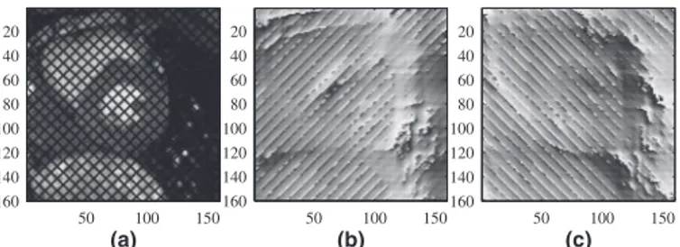
Fig. 1. (a) Tagged MR image with 45° and 135° tagging lines. (b) Phase imageφ1from

analytic signal s1, contains 45° tagging lines structural information. (c) Phase imageφ2

from analytic signal s2, contains 135° tagging lines structural information.

(d) ROI 76 81 86 91 58 63 68 73 -2 0 2 58 63 68 73 phase [rad] (c) Vertical [pixel] Vertical profile 76 81 86 91 -3 -2 -1 0 1 2 3 Horizontal [pixel] (b) phase [rad] Horizontal profile Horizontal [pixel] (a) Vertical [pixel] Phase image 50 100 150 20 40 60 80 100 120 140 160

Fig. 2. (a) Phase imageφ1from analytic signal s1with an ROI in the green rectangle.

(b) Horizontal profiles of two successive frames inφ1ROI in (d). (c) Vertical profile of

two successive frames inφ1ROI in (d). (d) ROI (zoomed in) ofφ1in (a) with

horizon-tal/vertical profile lines (green dashed lines).

the tagged MR image ofFig. 1, the tagging lines along two directions constitute two complementary structural information.

Although there exists a linear relation between the QS phases

φ

i,

φ

jand the AS phases

φ

1,

φ

2,

φ

3,

φ

4, while the QS phase

φ

kcontained

the modulus of AS (Hahn and Snopek, 2004, 2011), the QS phases do not split information in the two tagging line directions. This makes QS less suitable for calculating the spatial gradient of the phase needed in the next step of our method. Therefore, we use

φ

1,

φ

2of s1, s2in

Eqs. (5)and(6)as a basis for the myocardium displacement

estima-tion in our method.

Fig. 1shows the spatial phases obtained via the AS s1and s2, on a

tagged MR image with tagging lines along the 45° and 135° directions.

φ

1holds the structural information of the 45° tagging lines, while

φ

2

holds the ones of the 135° tagging lines. An example of the profile of phase

φ

1in a region of interest (ROI) ofFig. 1(b) is shown inFig. 2.

2.2. Optical flow method from the spatial phase images

The optical flow equation is largely used for motion estimation in various application domains. It is based on the assumption of pixel in-tensity conservation over time, and of small displacements between

consecutive frames (typically smaller than 1 pixel). Based on these hypothesis and using a Taylor series development of order 1, the op-tical flow equation is written as:

i(x, y, t)= i(x + dx,y + dy,t + dt

)

= i(x, y, t)+dx

∂i

∂x

+dy

∂i

∂y

+dt

∂i

∂t

+O

¡

d2 x,d2y,dt2

¢

⇔dx

∂i

∂

x+dy

∂i

∂

y+dt

∂

i

∂t

=0, (9)

where i is the intensity function of space (x, y) and time (t) variables, dxand dythe displacement of the pixel at position (x, y), dtthe

tem-poral sampling step, and O

(

d2

x,dy2,dt2

)

is the higher-order term. In the

following, without loss of generality, we use dt=1 in order to sim-plify the mathematical expressions.

In this paper, we propose replacing the intensity invariance as-sumption by the phase over time. Thus,Eq. (9)is replaced hereafter by two equations holding on the two phases

φ

1,

φ

2of AS s1and s2:

dx

∂φ

1

∂x

+dy

∂φ

1

∂y

+

∂φ

1

∂t

=0, dx

∂φ

2

∂x

+dy

∂φ

2

∂y

+

∂φ

2

∂t

=0. (10) Hence, dx, dy can be obtained by solving the previous system of two equations with two unknowns:

dx= ∂φ1 ∂y ∂φ2 ∂t − ∂φ2 ∂y ∂φ1 ∂t ∂φ1 ∂x ∂φ2 ∂y − ∂φ1 ∂y ∂φ2 ∂x , dy= ∂φ1 ∂x ∂φ2 ∂t − ∂φ2 ∂x ∂φ1 ∂t ∂φ1 ∂y ∂φ2 ∂x − ∂φ1 ∂x ∂φ2 ∂y , (11) where ∂φ1 ∂x, ∂φ₂ ∂x , ∂φ₁ ∂y, ∂φ₂

∂y are the spatial derivatives of

φ

1 and

φ

2

with respect to the spatial coordinates. The terms∂φ1

∂t and ∂φ₂

∂t are the

temporal derivatives of the phases. They may be classically calculated by finite difference numerical differentiation. We propose, in order to avoid the phase jumps problem and possible errors of phase unwrap-ping, computing the temporal derivatives of the phases directly from the AS and its conjugates:

∂φ

1

∂t

=Arg[s ∗ 1

(x, y, t)

·s1

(x, y, t + 1)

], (12)

∂φ

2

∂t

=Arg[s ∗ 2

(x, y, t)

·s2

(x, y, t + 1)

], (13) with s∗

1the conjugate of s1, and s∗2the conjugate of s2. In the

follow-ing, phases are computed usingEqs. (5)and(6)within local blocks extracted from tagged MR images and used to assess a local bilinear model.

2.3. Bilinear model of the local motion

Since the human myocardium has a relatively complex motion, the local displacement of myocardium cannot be estimated accu-rately by a simple rigid translation model. As a consequence, a more complex motion model is needed to approach local displacement bet-ter. In this paper, we used a bilinear model consisting of translation, dilation, rotation, and motion components. Such a model has already been used, for instance, for tissue displacement estimation in ultra-sound elastographic image sequences (Basarab et al., 2008).

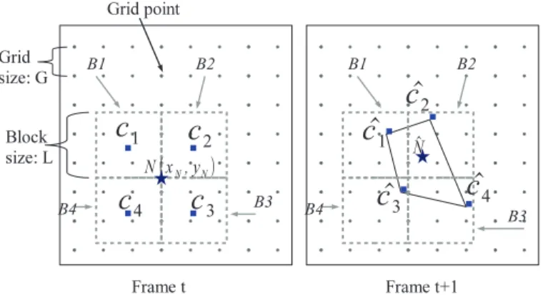
The basic principle is shown inFig. 3. First, a collection of nodes on a rectangular grid is considered in the reference frame. The dis-tance between two consecutive nodes is denoted by G inFig. 3. The displacement of each node (grid point) is estimated by considering a bilinear deformation of a rectangular region centered on the current node. The displacement of one grid point N(xN, yN) (star) between

frames t and t + 1, illustrated inFig. 3, is derived byEqs. (14)–(17). Let us define B1, B2, B3, B4 as the four blocks having in common the pixel N, and C1, C2, C3, C4the centers of the blocks B1, B2, B3, B4. By

Fig. 3. Displacement estimation between point N(xN, yN) (star) on frame t and point

ˆ

N on frame t + 1: Firstly, the displacement of four neighbor blocks B1, B2, B3, B4 of N

are estimated separately, the average motion vector of each block is used as its center displacement from cito ˆci(i = 1, 2, 3, 4). Next, the displacement of N to ˆN is calculated

by the bilinear model based on the position of ˆc1,cˆ2,cˆ3,cˆ4.

φ

1B,

φ

2B. Substituting intoEq. (11), we obtain the two displacement

components (dx(C), dy(C)): dx

(C)

= ∂φ1B ∂y ∂φ2B ∂t − ∂φ2B ∂y ∂φ1B ∂t ∂φ1B ∂x ∂φ2B ∂y − ∂φ1B ∂y ∂φ2B ∂x ,dy

(C)

= ∂φ1B ∂x ∂φ2B ∂t − ∂φ2B ∂x ∂φ1B ∂t ∂φ1B ∂y ∂φ2B ∂x − ∂φ1B ∂x ∂φ2B ∂y , (14) with ∂φ1B ∂t =Arg[s1B

(

x, y, t

)

·s∗1B

(

x, y, t + 1

)

], and ∂φ_2B ∂t =Arg[s2B

(

x, y, t

)

·s∗

2B

(

x, y, t + 1

)

]. Therefore, we obtain the displacements [dx(C1),

dy(C1)], [dx(C2), dy(C2)], [dx(C3), dy(C3)], and [dx(C4), dy(C4)] from

blocks B1, B2, B3, and B4, respectively. The displacement [dx(N), dy(N)]

of grid point N(xN, yN) can be calculated by the four displacements of

point C1, C2, C3, and C4as below. For this, the eight parameters of the

bilinear model are estimated as follows:









ax bx cx dx









=M









dx

(C

1

)

dx

(C

2

)

dx

(C

3

)

dx

(C

4

)









,









ay by cy dy









=M









dy

(C

1

)

dy

(C

2

)

dy

(C

3

)

dy

(C

4

)









, (15)

where the matrix M is depends on the block size L inFig. 3:

M = 1 2























−1 L 1 L 1 L − 1 L −1 L − 1 L 1 L 1 L 2 L2 − 2 L2 2 L2 − 2 L2 1 2 1 2 1 2 1 2























. (16)

Then, the displacement of point N(xN, yN) is obtained by:

dx

(N)

=axxN+bxyN+cxxNyN+dx,

dy

(N)

=ayxN+byyN+cyxNyN+dy. (17)

The detailed procedure is introduced in (Basarab et al., 2008). Once the displacements of all the grid points (separated by a distance of G larger than one pixel in the reference frame) are estimated, a 2D linear interpolation is employed to extend them to all the pixels of the image, resulting into a dense motion field (Basarab et al., 2008).

In order to improve the estimation accuracy, a global refining method is proposed in the following.

2.4. Refined model

For two successive images itand it+1,an initial estimation of the

displacement field

(

d0

x,d0y

)

is obtained as described in the previous

section:

£

d0 x

(x, y)

,d0y

(x, y)

¤

=

1

[it

(x, y)

,it+1

(x, y)

], (18)

where

1

is the motion estimator described inSection 2.3. Based on this motion field and the first image it(x, y), an inter-frame ˆi1_t+1

(

x, y

)

is generated by:

ˆi1

t+1

(x, y)

=it

¡

x + d0x

(x, y)

,y + dy0

(x, y)

¢

, (19)

where the new position of the pixel (x0, y0) in it(x, y) is [x0+

d0

x

(

x0,y0

)

,y0+dy0

(

x0,y0

)

] and each pixel value of ˆi1t+1

(

x, y

)

is

ob-tained by spline interpolation. Ideally, the generated image ˆi1

t+1

(

x, y

)

and the image it+1

(

x, y

)

should contain the same phase information. However, in practice, this is not true because of motion estimation errors. Therefore, a com-pensated motion field [d1

xc

(

x, y

)

,dyc1

(

x, y

)

] is estimated between

im-age ˆi1

t+1

(

x, y

)

and it+1

(

x, y

)

by the same bilinear phase-based optical

flow method proposed inSection 2.3:

£

d1 xc

(x, y)

,d1yc

(x, y)

¤

=

1

£

ˆi1t+1

(x, y)

,it+1

(x, y)

¤

. (20)

Then, the estimated motion field [dx(x, y), dy(x, y)] between two

successive images itand it+1with improved accuracy is obtained by:

dx

(x, y)

=d0x

(x, y)

+d1xc

(x, y)

,

dy

(x, y)

=d0y

(x, y)

+d1yc

(x, y)

. (21)

This process can be iterated a number of times leading to the iter-ative scheme:

dk

x

(x, y)

=dk−1x

(x, y)

+dkxc

(x, y)

,

dky

(x, y)

=dk−1y

(x, y)

+dkyc

(x, y)

, (22)

with k the iteration number (k ≥ 1). This iteration procedure is part of step 2 ofAlgorithm 1. (seeSection 2.5). With this iterative scheme, a more accurate motion field [dx(x, y), dy(x, y)] is obtained.

2.5. Algorithm implementation

The pseudo-code of the proposed motion estimation method be-tween two consecutive images is given inAlgorithm 1.

3. Results

The proposed method was evaluated on both synthetic and clini-cal data. First, 7 realistic simulated sequences were used to evaluate the accuracy of the proposed method compared to two existing ap-proaches. Second, 11 in vivo data sets from 9 patients and 2 healthy volunteers are presented to highlight the clinical relevance of the pro-posed method.

3.1. Simulated data

The proposed method was tested on different realistic tagged MRI sequences corresponding to a cardiac cycle, simulated with ASSESS software (Clarysse et al., 2011). With this simulator, a combination of thickening and rotations simulates the contraction over time within a short-axis MRI slice. It is also possible to introduce a local motion anomaly by reducing the myocardium contraction magnitude within a myocardial sector (Clarysse et al., 2000). Therefore, the ground truth motion data were used as a reference to evaluate the proposed method. Several simulations were generated by acting on the simu-lator parameters. Each simulation term inTable 1can be interpreted as follows: “256” or “160” for the size of each square frame in pixels, “D20” for contraction/expansion of 20%, “R20” for 20 degrees rota-tion, “F20” or “F34” for frame number of 20 or 34, and “P0” for healthy or “P3” for pathological state with the highest degree of the myocar-dial motion abnormality.

Algorithm 1 Phase-based bilinear block and compensation optical

flow.

Require: two subsequent frames: it

(

x, y

)

,it+1

(

x, y

)

.

parameter: G, L, kMax.

G: Grid distance for bilinear model in pixels on horizontal and vertical direction.

L: Block size for bilinear model in pixels on horizontal and vertical direction.

kMax: Maximum iteration number.

Ensure: Displacement [dx(x, y

)

,dy(x, y

)

] between it

(

x, y

)

and

it+1

(

x, y

)

. 1: Step 1:

2: for

(

x, y

)

=grid points coordinate on frame it do

3: for each of the four neighbour block of the current grid point do 4:

£

s1B

(

t

)

,s2B

(

t

)

,

φ

1B

(

t

)

,

φ

2B

(

t

)

¤

=BlockAS

(

B

(

t

))

. 5:

£

s1B

(

t + 1

)

,s2B

(

t + 1

)

,

φ

1B

(

t + 1

)

,

φ

2B

(

t + 1

)

¤

= BlockAS

(

B

(

t + 1

))

. {Eqs. (5),(6).} 6:

£

dx(C

)

,dy(C

)

¤

=PhaseOpticalFlow(s1B,s2B,

φ

1B,

φ

2B). {Eq. (14).} 7: end for

8: [dx(N

)

,dy(N

)

] = BilinearModel([dx

(

C

)

,dy(C

)

]). {Compute the displacement of the current grid point N.}

9: end for

10:

£

d0

x

(

x, y

)

,dy0

(

x, y

)

¤

=DenseMotion([dx(N

)

,dy(N

)

]).{Interpolation on all the grid point N to obtain dense motion field}

11: Step 2:

12: dk−1

x

(

x, y

)

=dx0

(

x, y

)

,dk−1y

(

x, y

)

=dy0

(

x, y

)

{initialize for refining interation k.}

13: for k = 1:kMax do

14: {kMax is the maximum iteration number}

15: ˆi_t+1k =ObjectFrameGeneration(dxk−1,dk−1y ,it). {Eq. (19).} 16: [dk

xc,dkyc] = CompensatedDisplacement(ˆikt+1,it+1).

{Repeat Step 1 by Eq. (20).}

17: dk x=dk−1x +dxck,dky=dyk−1+dkyc{Eq. (21).} 18: end for 19: dx(x, y

)

=dkMax x

(

x, y

)

,dy(x, y

)

=dkMaxy

(

x, y

)

3.2. Robustness of phase

It is well known that tagged MRI sequences suffer from the non respect of the pixel brightness constancy over time and and in partic-ular from the tag fadding effect. In order to evaluate the robustness of our method to these factors, we have also generated a sequence, de-noted by “160D30R20P3F34Lum” inTable 1, that takes into account both the tag fading effect, based on the tag generation method in (Wang et al., 2014), and the non respect of the pixel intensity conser-vation over time. Following the evaluation of the tag fading in clini-cal sequences, the simulated tags fade linearly up to 80% on the last image of the sequence compared to the first frame. Furthermore, in

each image of the sequence, we changed the intensity of the image by a random percentage value between 40% and 100% of the origi-nal intensity. In order to modify the intensity of each image of the sequence, we multiplied the original image by a 2D weighting im-age

(

a +

(

1 − a

)

G

(

x, y

))

,with G(x, y) a Gaussian function. The range of the 2D weighting image is (a, 1], where a is a random real value taken in [0.4, 1]. As the consequence, we obtain a sequence with the pixel intensity from 40% to 100% of the original image intensity. Here we chose the minimum value a = 0.4 for the purpose of retain-ing at least 40% intensity of the original images.

The sequence intensity changes locally in each frame due to the Gaussian function and also changes along the time axis due to the random value a. Given an image i1with the tag fading effect, the

out-put image i2obtained by the 2D weighting image

(

a +

(

1 − a

)

G

(

x, y

))

is:

i2

(x, y)

=

(a +

(

1 − a

)G(x, y))i

1

(x, y)

, (23)

where G

(

x, y

)

=exp

(

−(x−x0)2+(y−y0)2

2σ2

)

,with (x0, y0) and

σ

the center

peak position and the standard deviation of G(x, y), respectively. We vary the center peak position (x0, y0) linearly along the time axis,

which changes the brightest region on each frame in the sequence.

Fig. 4 shows an example: The image inFig. 4(b) is generated by

multiplying each pixel value by the corresponding pixel value of the 2D weighting function in Fig. 4(e) leading to a 20% intensity reduction in the myocardial region.

Figs. 4(c) and (d) display the phase images

φ

1given inEq. (5)

cal-culated from the images inFigs. 4(a) and (b), respectively. We note that both phase images hold the structural information and are less influenced by their varied intensity images.

3.3. Existing methods used for comparison

Taking into account the fact that the proposed method is based on the analytic signal and optical flow principles (more precisely on the phase flow), the evaluation results of an analytic signal estimator and optical flow estimator are presented for comparison purposes.

The first one is the Alessandrini monogenic signal method for the analysis of heart motion from medical images (Alessandrini et al., 2013). It outperforms the SinMod method (Arts et al., 2010) and was shown to be more accurate with less computation than another algo-rithm based on the monogenic signal (Zang et al., 2007).

The second method used for comparison is called Sun classic NL in (Sun et al., 2010). It was declared the best optical flow algorithm in 2010 in the Middlebury evaluation ranking (Baker et al., 2007; 2011) (used for the evaluation of optical flow algorithms), and in an ex-panded literature review in 2014 (Sun et al., 2014). This method was also reported to provide good results in the new optical evaluation datasets in 2012 such as KITTI (Geiger et al., 2012) (autonomous driv-ing platform to develop new benchmarks for the tasks of stereo, opti-cal flow, and 3D object detection) and MPI Sintel (Butler et al., 2012) (new optical flow data set derived from the open source 3D animated short film Sintel). Hence, these Alessadrini’s and Sun’s methods could be considered as suitable references. Publically available implemen-tations were used for both methods (Alessandrini, 2013; Sun, 2010).

Table 1

Eulerian average endpoint error (µ±σ) in pixels on seven simulated sequences and their computing time. Sequence Endpoint error [pixels] Computing time [min]

Proposed Alessandrini Sun classicNL Proposed Alessandrini Sun classicNL (1)256R20F20 0.050 ± 0.055 0.087 ± 0.064 0.089 ± 0.082 5.00 0.48 15.95 (2)256D30F20 0.015 ± 0.013 0.035 ± 0.025 0.036 ± 0.034 5.00 0.52 13.43 (3)256D30R20P0F20 0.063 ± 0.066 0.094 ± 0.069 0.092 ± 0.090 5.02 0.70 16.08 (4)256D30R20P3F20 0.062 ± 0.065 0.099 ± 0.075 0.097 ± 0.095 5.02 0.68 16.03 (5)160D30R20P0F34 0.035 ± 0.027 0.045 ± 0.025 0.048 ± 0.038 2.68 0.57 13.10 (6)160D30R20P3F34 0.034 ± 0.025 0.041 ± 0.022 0.045 ± 0.035 2.58 0.58 13.52 (7)160D30R20P3F34Lum 0.045 ± 0.032 0.048 ± 0.028 0.057 ± 0.043 2.77 0.63 16.67

50 100 150 20 40 60 80 100 120 140 160 0 50 100 150 200 250 (a) 50 100 150 20 40 60 80 100 120 140 160 0 50 100 150 200 250 (b) 50 100 150 20 40 60 80 100 120 140 160 -3 -2 -1 0 1 2 3 (c) 50 100 150 20 40 60 80 100 120 140 160 -3 -2 -1 0 1 2 3 (d) 50 100 150 20 40 60 80 100 120 140 160 0 0.2 0.4 0.6 0.8 1 (e)

Fig. 4. (a) A tagged MR image. (b) Image of 40% of tag fading from (a) with global 20% intensity reduction within the myocardial region obtained by the 2D weighting func-tion. (c) The phaseφ1of (a). (d) The phaseφ1of (b). (e) 2D weighting image from the

Gaussian function (σ=20,(x0,y0)=(59, 52),a = 0.80). The phase images (c) and (d)

contain highlighted structural information as compared to the corresponding intensity images (a) and (b).

3.4. Evaluation criteria

Angular error (AE) and endpoint error (EE) are common crite-ria used to evaluate the difference between the theoretical and esti-mated displacements. However, AE is less suitable for small displace-ments (Alessandrini et al., 2013) and the EE is a more appropriate measure of displacement vector accuracy (Baker et al., 2011). Hence, we used EE to evaluate the estimation accuracy. The EE at one loca-tion is defined as:

EE

(x, y)

=

p

(d

x

(x, y)

−dxr

(x, y))

2+

(d

y

(x, y)

−dyr

(x, y))

2, (24)

where [dxr(x, y), dyr(x, y)] are the ground truth reference

displace-ments along horizontal and vertical directions, respectively, and [dx(x,

y), dy(x, y)] are the estimated ones. The average and standard

devia-tions of EE for both Eulerian and Lagrangian displacements are com-puted to quantify the performance of the method. The EE values ob-tained for several simulation sequences results are presented and dis-cussed in the following sections.

3.5. Method parameters

The parameters for all the methods are determined based on the sequences in Table 1. With the proposed method, for the bilinear model, the grid distance is 4 × 4 pixels and the block size is 10 ×

10 pixels. To highlight this trade-off, we processed the motion estima-tion for all the seven simulated sequences for 1, 2, 3 and 4 refinement iterations. The average EE between the seven sequences was equal to 0.055, 0.042, 0.039, and 0.037 pixels, respectively.

The computing time to process all the seven sequences (80 im-ages of 256 × 256 pixels and 102 imim-ages of 160 × 160 pixels) is 18.59, 27.87, 37,18, 46.54 min, respectively, corresponding to 1, 2, 3 and 4 it-erations. With Alessandrini method, the optimized parameters pro-posed in (Alessandrini et al., 2013) are used, which are the initial wavelength

λ0

=4 and the refinement step number Np=5. For the

Sun classicNL method, we adopted the parameters recommended in

(Sun et al., 2010), which are the sobel edge detector with a mask of

5 × 5 pixels and a neighborhood of 15 × 15 pixels. 3.6. Eulerian motion estimation results

3.6.1. Global results for all simulation sequences

Table 1shows the EE results for the seven simulated sequences.

For each sequence, we calculate a spatial average EE value

µ

and the standard deviation

σ

.

All the methods were implemented in MATLAB (R2012b, The Math-Works, Natick, MA), on a laptop computer (CPU: Intel i7-4750HQ 2.0GHz, RAM: 16384MB).Table 1shows our results com-pared with the Alessandrini and Sun classicNL methods. Based on the summation of EE results of the seven sequences, the errors of the proposed method are reduced by 33% and 35% compared with that of the Alessandrini’s and Sun’s methods, respectively. On the variable intensity sequence “160D30R20P3F34Lum” and the constant intensity sequence “160D30R20P3F34,” the proposed method pro-vides a robust estimation. Besides, the proposed method is about 28% faster that Sun’s method while providing a better motion esti-mation result. Although the Alessandrini method is outperformed by the proposed method, it is less time-consuming than the two other approaches.

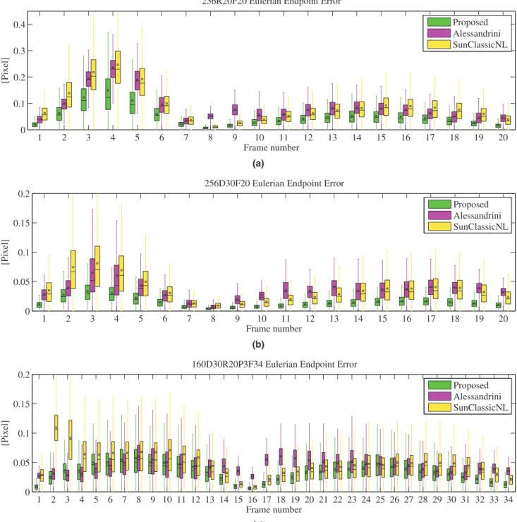
Fig. 5 presents a frame-by-frame EE comparison through

box and whiskers plots for three sequences. These sequences present different kinds of motions: pure rotation of sequence “256R20F20”, pure contraction/expansion of sequence “256D30F20”, and rotation+contraction/expansion+deformation of sequence “160D30R20P3F34”. The sequences “256R20F20” and “256D30F20” contain 7 frames in the systolic and 13 frames in the diastolic phase of one cardiac cycle. The sequence “160D30R20P3F34” contains 14 and 20 frames in the systolic and diastolic phase, respectively.

InFig. 5(a) and (b), it is clear that during the systolic phase (frame 1 to 7), which corresponds to the larger displacements and also the diastole phase (frame 8 to 20). The estimation results of the pro-posed method are much better than the other two methods. We obtain the smallest end point error on each frame from the pro-posed method. InFig. 5(c), during the systolic phase (frame 1 to 14), we obtain better estimation results with the proposed method than with the Sun classicNL method and almost equivalent estimation re-sults as the Alessandrini method. At the beginning of the diastolic phase, the proposed method provides similar performance as the Sun classicNL method. In the diastole (frame 16 to 34), the proposed method is more accurate than the other two methods. Especially, in the frames where the displacement is relatively small, the proposed method outperforms the Alessandrini method at the frames 16 to 23, and it also outperforms the Sun classicNL method at frames 27 to 34.

3.6.2. Detailed EE results from one test case sequence

Performances of the three methods were studied in details on sequence “160D30R20P3F34”, which presents one cardiac cycle represented by 14 frames in the systolic and 20 frames in the diastolic phase.Fig. 6compares the EE results between the three methods on a systolic frame and a diastolic frame. In the systolic frame result (first

1

2

3

4

5

6

7

8

9

10

11

12

13

14

15

16

17

18

19

20

0

0.1

0.2

0.3

0.4

Frame number

[Pixel]

256R20F20 Eulerian Endpoint Error

Proposed

Alessandrini

SunClassicNL

(a)

1

2

3

4

5

6

7

8

9

10

11

12

13

14

15

16

17

18

19

20

0

0.05

0.1

0.15

0.2

Frame number

[Pixel]

256D30F20 Eulerian Endpoint Error

Proposed

Alessandrini

SunClassicNL

(b)

1

2

3

4

5

6

7

8

9 10 11 12 13 14 15 16 17 18 19 20 21 22 23 24 25 26 27 28 29 30 31 32 33 34

0

0.05

0.1

0.15

0.2

Frame number

[Pixel]

160D30R20P3F34 Eulerian Endpoint Error

Proposed

Alessandrini

SunClassicNL

(c)

Fig. 5. Box and whiskers plots of Eulerian endpoint errors for sequences (a) “256R20F20”, (b) “256D30F20”, (c) “160D30R20P3F34”. Each box corresponds to the statistical

distri-bution of all EE values on one frame. The center bar of each box represents the median value. The circle indicates the average value, and the box body extends from the 25th to the 75th percentile of one frame of EE values.

row), the proposed method generates smaller error values. In the diastolic frame result (second row), there is no very clear observable difference between the three methods.

To better understand the performance of the methods, it is im-portant to analyze vertical and horizontal displacement separately. Accordingly,Fig. 7presents these results at frame 10, which has one of the largest displacements of two successive frames during the car-diac cycle. The ground truth motions are in the first row; the pro-posed method results, Alessandrini results, and Sun classicNL results are displayed in the second, third and fourth rows, respectively. dx

indicates the horizontal displacement (first column) with its abso-lute error map beside (second column). dyrepresents the vertical

dis-placement (third column) with its absolute error map on the right

(fourth column). The comparison of the absolute error in the second and third row highlights that the EE map is slightly smaller in mag-nitude for our method as compared to the Alessandrini method. Also, the proposed method error is much smoother than the Sun classicNL method error.

Fig. 8 presents frames 10 and 24 extracted from sequence

“160D30R20P3F34” of one cardiac cycle with a superposition of the Eulerian motion vector estimated within the frames 10–11 and 24–25. The frames 10 and 24 belong, respectively, to systole and diastole phases, with a corresponding cardiac time in terms of the percentage value of one cardiac cycle period. These motion vectors vary for each frame, thus allowing for a local observation of the movement within the myocardium.

Proposed (frame=10) 40 60 80 100 120 40 60 80 100 120 Alessandrini (frame=10) 40 60 80 100 120 40 60 80 100 120 SunClassicNL (frame=10) 40 60 80 100 120 40 60 80 100 120 0.05 0.1 0.15 0.2 0.25 0.3 0.35 Proposed (frame=24) 40 60 80 100 120 40 60 80 100 120 Alessandrini (frame=24) 40 60 80 100 120 40 60 80 100 120 SunClassicNL (frame=24) 40 60 80 100 120 40 60 80 100 120 0 0.05 0.1 0.15 0.2 0.25

Fig. 6. EE results of three methods (unit: pixels) of sequence “160D30R20P3F34”. First

row: systolic frame 10. Second row: diastolic frame 24. First column: proposed method. Second column: Alessandrini method. Third column: Sun classicNL method.

160D30R20P3F34 (frame=10) Ground Truth (Eulerian): dx

40 60 80 100 120 40 60 80 100 120 [Pixel] -1 -0.5 0 0.5 1 160D30R20P3F34 (frame=10) Ground Truth (Eulerian): dy

40 60 80 100 120 40 60 80 100 120 [Pixel] -1 -0.5 0 0.5 1 Proposed: dx (frame=10) 40 60 80 100 120 40 60 80 100 120 abs Error: dx 40 60 80 100 120 40 60 80 100 1200 0.1 0.2 0.3 Proposed: dy (frame=10) 40 60 80 100 120 40 60 80 100 120 abs Error: dy 40 60 80 100 120 40 60 80 100 1200 0.1 0.2 0.3 Alessandrini: dx (frame=10) 40 60 80 100 120 40 60 80 100 120 abs Error: dx 40 60 80 100 120 40 60 80 100 1200 0.1 0.2 0.3 Alessandrini: dy (frame=10) 40 60 80 100 120 40 60 80 100 120 abs Error: dy 40 60 80 100 120 40 60 80 100 1200 0.1 0.2 0.3 SunClassicNL: dx (frame=10) 40 60 80 100 120 40 60 80 100 120 abs Error: dx 40 60 80 100 120 40 60 80 100 1200 0.1 0.2 0.3 SunClassicNL: dy (frame=10) 40 60 80 100 120 40 60 80 100 120 abs Error: dy 40 60 80 100 120 40 60 80 100 1200 0.1 0.2 0.3

Fig. 7. Displacement and absolute value error map in pixels of sequence

“160D30R20P3F34” for three motion estimation methods. The horizontal displacement in pixels and its error are in the first column and second column, respectively. The ver-tical displacement in pixels and its absolute error are in the third and fourth columns, respectively. First row: the ground truth. Second row: the proposed method. Third row: Alessandrini method. Fourth row: Sun classicNL method.

3.7. Lagrangian motion estimation results

The Lagrangian motion field represents the spatial displacement of material points in the reference state (first frame) along time. This spatio-temporal Lagrangian displacement field [uL(x, y), vL(x, y)] can

be recovered through forward integration of the Eulerian motion field [dx(x, y), dy(x, y)]. For a motion field between time t and t + 1, we

cal-culate the Lagrangian motion field [uL

(

x, y, t + 1

)

,

v

_L

(

x, y, t + 1

)

] from

the Lagrangian motion field [uL(x, y, t), vL(x, y, t)] at time t and the

Eu-lerian motion field [dx(x, y, t + 1

)

,dy(x, y, t + 1

))

] at time t + 1:

uL

(x, y, t + 1)

=uL

(x + d

x

(x, y, t + 1)

,y + dy

(x, y, t + 1)

,t), (25)

Max vector=1.2[pixels];AMP=8;Frame=10 Time=29% of one cardiac cycle.

(a)

Max vector=0.96[pixels];AMP=8;Frame=24 Time=69% of one cardiac cycle.

(b)

Fig. 8. The Eulerian estimated motion vectors of sequence “160D30R20P3F34” from

the proposed method. (a) Frames 10 from systole. (b) Frame 24 from diastole. Motion vectors are amplified by a factor of 8. The cardiac time of each frame is presented in terms of the percentage of a whole cardiac cycle.

v

_L

(x, y, t + 1)

=

v

_L

(x + d

_x

(x, y, t + 1)

,y + dy

(x, y, t + 1)

,t), (26)

with the initial conditions uL

(

x, y, 1

)

=dx

(

x, y, 1

)

,

v

_L

(

x, y, 1

)

= dy(x, y, 1

)

. A bilinear interpolation is applied on the four neighbour points of the current point to calculate the motion field uL

(

x +

dx

(

x, y, t + 1

)

,y + dy(x, y, t + 1

)

,t

)

and

v

_L(x + d_x

₍

x, y, t + 1

₎

,y + dy(x, y, t + 1

)

,t

)

.

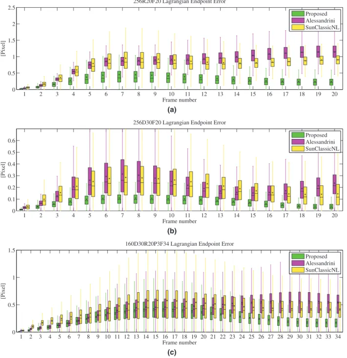
Fig. 9shows the Lagrangian EE of each frame through box and

whiskers plots for the three sequences inFig. 5. As expected, the es-timation errors of the Lagrangian motion fields are accumulated over time from the Eulerian errors inFig. 5. The level of error of the pro-posed method is less than 0.5, 0.1 and 0.5 pixel, respectively. As high-lighted inFigs. 5and9, our method outperforms the two other ap-proaches in the estimation of Lagrangian motion fields.

One major indicator for cardiac function diagnosis is represented by the myocardial strains (Qian et al., 2011), which can be computed from spatial derivatives (processed using standard smooth numer-ical differentiation in our work) of the Lagrangian accumulated motion field u = [uL

(

x, y, t

)

,

v

_L

(

x, y, t

)

] with respect to time. The

Green–Lagrange strain tensor is defined as:

E =1

2

¡∇

u +

∇

u

T₊

_∇

_uT

_∇

_u

¢

1 2 3 4 5 6 7 8 9 10 11 12 13 14 15 16 17 18 19 20 0 0.5 1 1.5 2 2.5 Frame number [Pixel]

256R20F20 Lagrangian Endpoint Error

Proposed Alessandrini SunClassicNL

(a)

1 2 3 4 5 6 7 8 9 10 11 12 13 14 15 16 17 18 19 20 0 0.1 0.2 0.3 0.4 0.5 0.6 Frame number [Pixel]

256D30F20 Lagrangian Endpoint Error

Proposed Alessandrini SunClassicNL

(b)

1 2 3 4 5 6 7 8 9 10 11 12 13 14 15 16 17 18 19 20 21 22 23 24 25 26 27 28 29 30 31 32 33 34 0 0.5 1 1.5 Frame number [Pixel]

160D30R20P3F34 Lagrangian Endpoint Error

Proposed Alessandrini SunClassicNL

(c)

Fig. 9. Box and whiskers plots of Lagrangian endpoint errors for sequences (a) “256R20F20”, (b) “256D30F20”, (c) “160D30R20P3F34”. Each box corresponds to the statistical

distribution of all EE values on one frame. The center bar of each box represents the median value. The circle indicates the average value, and the box body extends from the 25th to the 75th percentile of one frame of EE values.

where,

∇

is the spatial derivative operator and uT_{is the transpose of}

u. Furthermore, the radial deformation Erralong direction r and

cir-cumferential deformation Eccalong direction c can be obtained by:

Err=rTEr, Ecc=cTEc. (28)

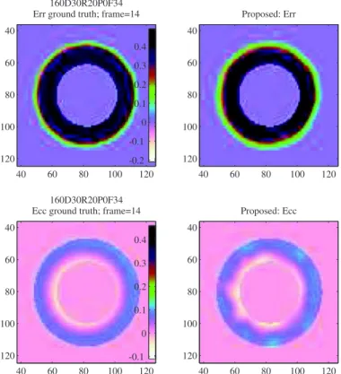
In the simulated sequences “160D30R20P0F34” and “160D30R20P3F34,” the systolic (from frame 1 to end-systolic frame 14) radial and circumferential strains were computed.

Fig. 10shows the myocardial deformation at frame 14 of sequence

“160D30R20P0F34.” The uniformity of deformation is observable in this healthy case from both the ground truth and proposed method results.

Fig. 11shows the radial and circumferential strains for the

patho-logical case (sequence “160D30R20P0F34”). The four columns are

in the order of the ground truth, the proposed method result, the Alessandrini result, and the Sun classicNL result. A simulated pathol-ogy region is located in the upper left region of the myocardium (in-dicated by an arrow in the figure). From the radial deformation re-sults Err, all three methods can recover the pathology, while from the

circumferential deformation results, our proposed method obtains a more accurate pathology location than the other two methods. 3.8. Clinical results

This section is structured as follows. First, an in-depth analysis of 2 pathological cases and 1 healthy volunteer is presented. It aims at showing the effectiveness of our motion estimation technique in highlighting cardiac diseases through standard strain images

160D30R20P0F34 Err ground truth; frame=14

40 60 80 100 120 40 60 80 100 120 -0.2 -0.1 0 0.1 0.2 0.3 0.4 160D30R20P0F34 Ecc ground truth; frame=14

40 60 80 100 120 40 60 80 100 120 -0.1 0 0.1 0.2 0.3 0.4 Proposed: Err 40 60 80 100 120 40 60 80 100 120 Proposed: Ecc 40 60 80 100 120 40 60 80 100 120

Fig. 10. Estimated systolic myocardial strains in healthy case sequence. First row:

ra-dial deformation Err. Second row: circumferential deformation Ecc. First column: the

ground truth. Second column: the proposed method results.

160D30R20P3F34 Err ground truth; frame=14

40 60 80 100 120 40 60 80 100 120 -0.2 -0.1 0 0.1 0.2 0.3 0.4 160D30R20P3F34 Ecc ground truth; frame=14

40 60 80 100 120 40 60 80 100 120 -0.1 0 0.1 0.2 0.3 0.4 Proposed: Err 40 60 80 100 120 40 60 80 100 120 Proposed: Ecc 40 60 80 100 120 40 60 80 100 120 Alessandrini: Err 40 60 80 100 120 40 60 80 100 120 Alessandrini: Ecc 40 60 80 100 120 40 60 80 100 120 SunClassicNL: Err 40 60 80 100 120 40 60 80 100 120 SunClassicNL: Ecc 40 60 80 100 120 40 60 80 100 120

Fig. 11. Estimated systolic myocardial strains for the pathological case sequence

“160D30R20P3F34”. First row: radial deformation Err. Second row: circumferential

de-formation Ecc. The four columns are in the order of the ground truth, the proposed

method result, Alessandrini result, and Sun classicNL result, receptively.

and proposed motion trajectories. Second, 8 other in vivo image sequences from 7 patients and 1 healthy volunteer are presented to confirm the interest of motion trajectories in cardiac applications. A discussion on the correlation between radial deformation and the estimated endocardial and epicardial traces is provided for these 8 clinical cases.

3.8.1. Detailed analysis of two pathological cases

In this section, we applied our method to in vivo clinical sequences of pathological cases from a female patient (43 years old) and a male patient (65 years old).

Pathological case #1. This 43 year-old female acute myocardial in-farction (AMI) patient was hospitalized with a left anterior de-scending (LAD) occlusion, with a reperfusion performed H + 2. MR

(a)

(b)

Fig. 12. Selected images of patient #1. (a) Short-axis tagged MR image. Frame 1

(end-diastolic phase) of this sequence that was used to estimate the motion field; (b) image of LGE sequence with an area (edema in hypersignal) in the A, AS, and IS segments. A indicates anterior; AS, anteroseptal; IS, inferoseptal; I, inferior; IL, inferolateral; AL, anterolateral.

imaging was performed 5 days after reperfusion. The standard car-diovascular magnetic resonance (CMR) examination contained MR tagging and post-Gadolinium injection (10 min) with a 3D inversion-recovery gradient echo sequence. MR tagging was performed on a Siemens Avento 1.5T in short-axis and long-axis views with the fol-lowing parameters: gradient echo (GRE) sequence with 45° spatial modulation of magnetization (SPAMM) tagging pattern, TE = 1.39 ms, TR = 26.4 ms, flip angle = 20°, tag spacing = 6 mm, spatial resolu-tion = 1 × 1 mm, 21 frames, temporal resoluresolu-tion = 30 ms.

Fig. 12(a) shows the first frame (end-diastolic phase) of a

short-axis tagged slice located between the mid and apical level of the left ventricle. The myocardium is divided following the American Heart Association (AHA) segmentation (Cerqueira et al., 2002).Fig. 12(b) shows the late gadolinium enhancement (LGE) image at the same slice level. AMI appears as hyper-enhanced regions (AS, A, and IS seg-ments) with dark regions in the sub-endocardial layers correspond-ing to no-reflow regions.

Applying the proposed method to this clinical tagged MRI se-quence, the Lagrangian motion field is obtained by accumulating the Eulerian motion field.Fig. 13represents the Lagrangian motion field and the radial deformation (Err) at frame 13 (end-systole,

correspond-ing to the maximum contraction). InFig. 13(a), the amplitude of the movement in the A, AS, and IS segments are visibly smaller than in the AL, IL, and I segments, which is obviously in concordance with the lo-cation of the pathology. Due to the myocardial thickening during sys-tole, radial strain is usually positive in normal myocardium.Fig. 13(b) shows the reduced, and even negative, Errvalues in the pathological

anterior region.

Lagrangian material point trajectories in millimeters are displayed

inFig. 14. They provide a visual experience of the myocardium local

motion trace. Several locations are chosen on the first image of the sequence as the desired tracking points. From the short-axis image inFig. 14, we highlight clearly that during the cardiac cycle, the AS segment has decreased motion than other segments in adjacent or remote myocardium. Hence, these tracking results are able to give an alternative illustration of the pathologies.

Pathological case #2. This second clinical case illustrates an inferior AMI in a 65 year-old male (right coronary occlusion - reperfusion H + 5). Imaging was performed before discharge of the patient at day 5. A short-axis tagged MRI was performed on a Siemens Avento 1.5T with the following parameters: GRE sequence with 45° SPAMM tag-ging pattern, TE = 1.53 ms, TR = 36.4 ms, flip angle = 20°, tag spac-ing = 6 mm, spatial resolution = 1 × 1 mm, 21 frames, temporal resolution = 36.4 ms.

Fig. 13. (a) Lagrangian motion field at end-systole frame 13 (with 1.5 magnification

factor). (b) Radial strain Errat end-systole. The white regions (with reduced and

neg-ative values) in the A, AS and IS segments are matching the location of infarcted seg-ments.

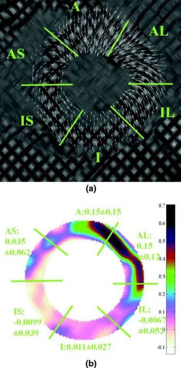
Fig. 15(a) shows the end-diastolic frame of the short-axis tagged

MR sequence at the mid level of the left ventricle.Fig. 15(b) shows the LGE image at the same slice level as the tagged image inFig. 15(a). Abnormal segments corresponding to myocardial necrosis are includ-ing the IS, I, and IL segments, with again, presence of no-reflow (sub-endocardial hyposignal) in the I and IL segments.

The estimated end-systolic motion field inFig. 16(a) shows that the myocardium is almost divided in two parts: the upper one (ante-rior) with a centripetal movement of normal amplitude, and the in-ferior wall with a major decrease of amplitude. The radial strain map inFig. 16(b) illustrates also the contrast between anterior and infe-rior parts of the circumference of the myocardium. In the IS, I, and IL segments, most of the negative deformation values and small positive values can be found in the lower part of the myocardium.

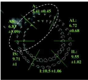
Fig. 14. MR tagging-based material point trajectories in millimeters for patient #1.

Short-axis view, note the reduced magnitude of motion in infarcted regions in the white dashed circle as compared to adjacent and remote regions. The white dashed circle delineates the regions with decreased motion in this antero-septo-apical infarc-tion. The mean length ± the standard deviation of the trajectories for each sector are provided.

Fig. 15. Selected images of patient #2. (a) Short-axis tagged MR image. Frame 1

(end-diastolic phase) of this sequence that was used to estimate the motion field. (b) Cor-responding slice of the LGE sequence showing an inferior infarction (hyper-enhanced regions) with no-reflow segments.

The Lagrangian material point trajectories in millimeters in

Fig. 17(a) give a global view of the whole sequence along time. In

the remote anterior regions A and AL segments (mostly), traces are smooth and large in amplitude. In the abnormal segments delineated with the dashed circle, traces are twisted and short, which demon-strate the lack of contractile capabilities in this acutely infarcted re-gions. We should remark that in other clinical cases long point tra-jectories may occur in infarcted regions due to passive motion (with low deformation) of these pathological sectors. A discussion on this effect is provided in the next section. In order to better highlight the difference between the tracking results of the healthy case and the pathological myocardial region of patient #2,Fig. 17(b) presents the tracking results of a healthy myocardium from a male volunteer. We can see from this healthy case that all the tracked points have uni-form contraction and dilation motions, which are different from the motion behavior of the pathological cases.

3.8.2. Discussion on the correlation between strain images and Lagrangian trajectories

The three in vivo data sets (two patients and one healthy volun-teer) detailed inSection 3.8.1 allowed us on one hand to validate the proposed motion estimation technique and on the other hand to highlight the possible contribution of Lagrangian trajectories to cardiac pathology diagnosis. For these two particular cases, an inter-esting correlation between the trajectories length and form and the

Fig. 16. (a) Lagrangian motion field at end-systole frame. (b) Radial deformation Errof

(a).

strain images was observed. In this section, results on seven addi-tional patients and on a second healthy volunteer are reported. The motion estimation and the strain image computation were processed in the same manner and with the same parameters as previously.

Figs. 18–25show the strain images and the endocardium and

epi-cardium trajectories (in millimeters) superimposed to the tagged MR images. For each myocardium segment, the mean and standard de-viation values are provided both for radial deformation and for La-grangian trajectories.

A qualitative observation confirms our initial findings: the motion trajectories are globally longer and more uniform for the healthy case than for the pathological ones. Moreover, the motion trajectories are generally shorter for the sectors with low deformation. However, as

(a)

(b)

Fig. 17. Trace of the myocardium local points on short-axis image sequence in

mil-limeters. (a) The region in the white dashed ellipse of the myocardium has shorter and non-smooth traces as compared to normal region at the myocardium segments A and AL, which indicates a potential impaired region. (b) Healthy volunteer #1. All the tracing points represent the same tendency of contraction/dilation.

(a) Radial deformation (b) Endocardial and epicardial traces

Fig. 18. Pathological case #3.

suggested inSection 3.8.1, passive motion may occur in such sectors, generating long motion trajectories. This is for example the case for sectors I and IL of patient #3 (seeFig. 18). The trajectory mean length in these sectors is indeed higher than the one in sector AS, while the AS radial deformation is considerably higher than in regions I and IL. However, we may remark that the trajectory standard deviation

(a) Radial deformation (b) Endocardial and epicardial traces

Fig. 19. Pathological case #4.

(a) Radial deformation (b) Endocardial and epicardial traces

Fig. 20. Pathological case #5.

(a) Radial deformation (b) Endocardial and epicardial traces

Fig. 21. Pathological case #6.

(a) Radial deformation (b) Endocardial and epicardial traces

Fig. 22. Pathological case #7.

(a) Radial deformation (b) Endocardial and epicardial traces

Fig. 23. Pathological case #8.

(a) Radial deformation (b) Endocardial and epicardial traces

Fig. 24. Pathological case #9.

(a) Radial deformation (b) Endocardial and epicardial traces

Fig. 25. Healthy volunteer #2.

values in I and IL sectors are roughly twice smaller than in AS, thus in agreement with the strain image.

These initial results are encouraging and suggest that material point motion trajectories may bring supplementary information to standard strain images in cardiac MRI. Further study on the clinical relevance of motion trajectories is of course necessary but out of the scope of this paper.

4. Discussions and conclusion

This paper introduced a motion estimation method for tagged MRI sequences based on the 2D single quadrant AS phases and the opti-cal flow method. The estimation accuracy of both Eulerian and La-grangian motion fields is improved compared to two approaches re-cently proposed in the literature.This improvement is mainly due to