3D shape of asteroid (6)~Hebe from VLT/SPHERE imaging: Implications for the origin of ordinary H chondrites

(1)

May 31, 2017

3D shape of asteroid (6) Hebe from VLT/SPHERE imaging:

Implications for the origin of ordinary H chondrites

?

M. Marsset

1

_{, B. Carry}

2, 3

_{, C. Dumas}

4

_{, J. Hanuš}

5

_{, M. Viikinkoski}

6

_{, P. Vernazza}

7

_{, T. G. Müller}

8

_{, M. Delbo}

2

_{, E. Jehin}

9

_,

M. Gillon

9

_{, J.Grice}

2, 10

_{, B. Yang}

11

_{, T. Fusco}

7, 12

_{, J. Berthier}

3

_{, S. Sonnett}

13

_{, F. Kugel}

14

_{, J. Caron}

14

_{, and R. Behrend}

14

1 _{Astrophysics Research Centre, Queen’s University Belfast, BT7 1NN, UK}

e-mail: michael.marsset@qub.ac.uk

2 _{Université Côte d’Azur, Observatoire de la Côte d’Azur, Lagrange, CNRS, France}

3 _{IMCCE, Observatoire de Paris, PSL Research University, CNRS, Sorbonne Universités, UPMC Univ Paris 06, Univ. Lille, France} 4 _{TMT Observatory, 100 W. Walnut Street, Suite 300, Pasadena, CA 91124, USA}

5 _{Astronomical Institute, Faculty of Mathematics and Physics, Charles University, V Holešoviˇckách 2, 18000 Prague, Czech}

Re-public

6 _{Department of Mathematics, Tampere University of Technology, PO Box 553, 33101 Tampere, Finland} 7 _{Aix Marseille Univ, CNRS, LAM, Laboratoire d’Astrophysique de Marseille, Marseille, France} 8 _{Max-Planck-Institut für extraterrestrische Physik, Giessenbachstrasse, 85748 Garching, Germany}

9 _{Space sciences, Technologies and Astrophysics Research Institute, Université de Liège, Allée du 6 Août 17, 4000 Liège, Belgium} 10 _{Open University, School of Physical Sciences, The Open University, MK7 6AA, UK}

11 _{European Southern Observatory (ESO), Alonso de Córdova 3107, 1900 Casilla Vitacura, Santiago, Chile} 12 _{ONERA - the French Aerospace Lab, F-92322 Châtillon, France}

13 _{Planetary Science Institute, 1700 East Fort Lowell, Suite 106, Tucson, AZ 85719, USA}

14 _{CdR & CdL Group: Lightcurves of Minor Planets and Variable Stars, Observatoire de Genève, CH-1290 Sauverny, Switzerland}

Received XXX; accepted XXX

ABSTRACT

Context.The high-angular-resolution capability of the new-generation ground-based adaptive-optics camera SPHERE at ESO VLT

allows us to assess, for the very first time, the cratering record of medium-sized (D∼100-200 km) asteroids from the ground, opening the prospect of a new era of investigation of the asteroid belt’s collisional history.

Aims.We investigate here the collisional history of asteroid (6) Hebe and challenge the idea that Hebe may be the parent body of

ordinary H chondrites, the most common type of meteorites found on Earth (∼34% of the falls).

Methods.We observed Hebe with SPHERE as part of the science verification of the instrument. Combined with earlier

adaptive-optics images and optical light curves, we model the spin and three-dimensional (3D) shape of Hebe and check the consistency of the derived model against available stellar occultations and thermal measurements.

Results.Our 3D shape model fits the images with sub-pixel residuals and the light curves to 0.02 mag. The rotation period (7.274 47 h),

spin (ECJ2000 λ,β of 343◦_,+47◦_{), and volume-equivalent diameter (193 ± 6 km) are consistent with previous determinations and}

thermophysical modeling. Hebe’s inferred density is 3.48 ± 0.64 g.cm−3_{, in agreement with an intact interior based on its H-chondrite}

composition. Using the 3D shape model to derive the volume of the largest depression (likely impact crater), it appears that the latter is significantly smaller than the total volume of close-by S-type H-chondrite-like asteroid families.

Conclusions.Our results imply that (6) Hebe is not the most likely source of H chondrites. Over the coming years, our team will

collect similar high-precision shape measurements with VLT/SPHERE for ∼40 asteroids covering the main compositional classes, thus providing an unprecedented dataset to investigate the origin and collisional evolution of the asteroid belt.

Key words. Minor planets, asteroids: individual (6 Hebe) – Meteorites, meteors, meteoroids – Techniques: imaging, lightcurves

1. Introduction

Disk-resolved imaging is a powerful tool to investigate the ori-gin and collisional history of asteroids. This has been remark-ably illustrated by fly-by and rendezvous space missions ( Bel-ton et al.,1992,1996;Zuber et al.,2000;Fujiwara et al.,2006;

Sierks et al.,2011;Russell et al.,2012,2016), as well as obser-vations from the Earth (e.g.,Carry et al. 2008,2010b;Merline et al. 2013). In the late nineties, observations of (4) Vesta with the Hubble Space Telescope (HST) led to the discovery of the now-called “Rheasilvia basin” and allowed for establishment of

? _{Based on observations made with ESO Telescopes at the La Silla}

Paranal Observatory under programme ID 60.A-9379 and 086.C-0785.

the origin of the Vestoids and HED meteorites found on Earth (Thomas et al., 1997;Binzel et al.,1997). Specifically, it was demonstrated that the basin-forming event on Vesta excavated enough material to account for the family of small asteroids with spectral properties similar to Vesta. HST observations thus con-firmed the origin of these bodies as fragments from Vesta, as pre-viously suspected based on spectroscopic measurements (Binzel & Xu, 1993). Recently, the Rheasilvia basin was revealed in much greater detail by the Dawn mission, which unveiled two overlapping giant impact features (Schenk et al.,2012a).

In the 2000’s, a new generation of ground-based imagers with high-angular-resolution capability, such as NIRC2 ( Wiz-inowich et al.,2000;van Dam et al.,2004) on the W. M. Keck II

(2)

telescope and NACO (Lenzen et al.,2003;Rousset et al.,2003) on the European Southern Observatory (ESO) Very Large Tele-scope (VLT), made disk-resolved imaging achievable from the ground for a larger number of medium-sized (∼100-200-km in diameter) asteroids. In turn, these observations triggered the de-velopment of methods for modeling the tridimensional shape of these objects by combining the images with optical light curves (see, e.g.,Carry et al. 2010a,2012;Kaasalainen et al. 2011; Vi-ikinkoski et al. 2015a). These models were subsequently vali-dated by in-situ measurements performed by the ESA Rosetta mission during the fly-by of asteroid (21) Lutetia (Sierks et al.,

2011;Carry et al.,2010b,2012;O’Rourke et al.,2012). More recently, the newly commissioned VLT/Spectro-Polarimetric High-contrast Exoplanet Research instrument (SPHERE) and its very high performance adaptive optics sys-tem (Beuzit et al.,2008) demonstrated its ability to reveal in even greater detail the surface of medium-sized asteroids by resolving their largest (D>30km) craters (Viikinkoski et al.,2015b;Hanuš et al.,2017). This remarkable achievement opens the prospect of a new era of exploration of the asteroid belt and its collisional history.

Here, we use VLT/SPHERE to investigate the shape and topography of asteroid (6) Hebe, a large main-belt asteroid (D∼180-200 km; e.g.,Tedesco et al.,2004;Masiero et al.,2011) that has long received particular attention from the commu-nity of asteroid spectroscopists, meteoricists, and dynamicists. Indeed, Hebe’s spectral properties and close proximity to or-bital resonances in the asteroid belt make it a possible main source of ordinary H chondrites (i.e., ∼34% of the meteorite falls, Hutchison 2004; Farinella et al. 1993; Migliorini et al. 1997; Gaffey & Gilbert 1998; Bottke et al. 2010). It was fur-ther proposed that Hebe could be the parent body of an ancient asteroid family (Gaffey & Fieber-Beyer,2013). The idea of H chondrites mainly originating from Hebe, however, was recently weakened by the discovery of a large number of asteroids (in-cluding several asteroid families) with similar spectral proper-ties (hence composition,Vernazza et al.,2014). Here, we chal-lenge this hypothesis by studying the three-dimensional shape and topography of Hebe derived from disk-resolved observa-tions. We observed Hebe throughout its rotation in order to de-rive its shape, and to characterize the largest craters at its surface. When combined with previous adaptive-optics (AO) images and light curves (both from the literature and from recent optical ob-servations by our team), these new obob-servations allow us to de-rive a reliable shape model and an estimate of Hebe’s density based on its astrometric mass (i.e., the mass derived from the study of planetary ephemeris and orbital deflections). Finally, we analyse Hebe’s topography by means of an elevation map and discuss the implications for the origin of H chondrites.

2. Observations and data pre-processing

We observed (6) Hebe close to its opposition date while it was orientated “equator-on” (from its spin solution derived below), that is, with an ideal viewing geometry exposing its whole sur-face as it rotated. Observations were acquired at four different epochs between December 8-12, 2014, such that the variation of the sub-Earth point longitude was 90±30◦_{between each epoch.}

Observations were performed with the recently commis-sioned second-generation SPHERE instrument, mounted at the European Southern Observatory (ESO) Very Large Telescope (VLT) (Fusco et al.,2006;Beuzit et al.,2008), during the

sci-ence verification of the instrument1_{. We used IRDIS}

broad-band classical imaging in Y (filter central wavelength=1.043 µm, width=0.140 µm) in the pupil-tracking mode, where the pupil re-mains fixed while the field orientation varies during the observa-tions, to achieve the best point-spread function (PSF) stability. Each observational sequence consisted in a series of ten images with 2 s exposure time during which Hebe was used as a natu-ral guide star for AO corrections. Observations were performed under average seeing conditions (0.9-1.100_{) and clear sky} trans-parency, at an airmass of ∼1.1.

Sky backgrounds were acquired along our observations for data-reduction purposes. At the end of each sequence, we ob-served the nearby star HD 26086 under the exact same AO con-figuration as the asteroid to estimate the instrument PSF for de-convolution purposes. Finally, standard calibrations, which in-clude detector flat-fields and darks, were acquired in the morning as part of the instrument calibration plan.

Data pre-processing of the IRDIS data made use of the preliminary release (v0.14.0-2) of the SPHERE data reduc-tion and handling (DRH) software (Pavlov et al., 2008), as well as additional tools written in the Interactive Data Lan-guage (IDL), in order to perform background subtraction, flat-fielding and bad-pixel correction. The pre-processed im-ages were then aligned one with respect to the others using the IDL ML_SHIFTFINDER maximum likelihood function, and averaged to maximise the signal to noise ratio of the asteroid. Finally, the optimal angular resolution of each image (λ/D=0.026", corresponding to a projected distance of 22 km) was restored with Mistral, a myopic deconvolution algorithm optimised for images with sharp boundaries (Fusco et al.,2002;

Mugnier et al., 2004), using the stellar PSF acquired on the same night as our asteroid data.

1 _{Observations obtained under ESO programme ID 60.A-9379 (P.I. C.}

(3)

Table 1. Date, mid-observing time (UTC), heliocentric distance (∆) and range to observer (r), phase angle (α), apparent size (Θ), longitude (λ) and latitude (β) of the subsolar and subobserver points (SSP, SEP). PIs of these observations were1_{J.-L. Margot,}2_{W. J. Merline,}3_{W. M. Keck}

engineering team,4_{F. Marchis,}5_{B. Carry, and}6_{C. Dumas.}

Date UTC Instrument ∆ r α Θ SEPλ SEPβ SSPλ SSPβ

(AU) (AU) (◦₎ ₍00₎ ₍◦₎ ₍◦₎ ₍◦₎ ₍◦₎ 1 2002-05-07 14:08:54 Keck/NIRC21 _2.52 _{1.88 20.5 0.131} _66.1 _-34.4 _{53.3 -17.4} 2 2002-05-08 13:55:01 Keck/NIRC21 _2.52 _{1.86 20.4 0.119 329.8} _{-34.5 317.2 -17.5} 3 2002-09-27 06:29:51 Keck/NIRC22 _2.21 _{1.91 27.0 0.098 162.5} _{-19.4 187.2 -35.4} 4 2007-12-15 14:15:39 Keck/NIRC23 _2.47 _{1.86 20.8 0.149} _14.2 _{32.9 356.2} _19.6 5 2007-12-15 14:30:31 Keck/NIRC23 _2.47 _{1.86 20.8 0.145} _1.9 _{32.9 343.9} _19.6 6 2007-12-15 14:44:49 Keck/NIRC23 _2.47 _{1.86 20.8 0.145 350.1} _{32.9 332.1} _19.6 7 2007-12-15 15:00:54 Keck/NIRC23 _2.47 _{1.86 20.8 0.138 336.8} _{32.9 318.9} _19.6 8 2007-12-15 15:27:39 Keck/NIRC23 _2.47 _{1.86 20.8 0.143 314.8} _{32.9 296.8} _19.6 9 2007-12-15 16:26:58 Keck/NIRC23 _2.47 _{1.86 20.8 0.151 265.9} _{32.9 247.9} _19.6 10 2009-06-07 10:52:24 Keck/NIRC22 _2.81 _{2.01 15.1 0.129} _43.1 _8.0 _57.9 _4.9 11 2010-06-28 13:08:00 Keck/NIRC24 _2.06 _{1.62 28.9 0.168 258.8} _{-39.3 221.2 -39.0} 12 2010-08-26 12:47:10 Keck/NIRC23 _1.98 _{1.05 16.1 0.260} _48.5 _-27.4 _{30.6 -31.2} 13 2010-08-26 13:04:26 Keck/NIRC23 _1.98 _{1.05 16.1 0.260} _34.3 _-27.4 _{16.3 -31.2} 14 2010-08-26 13:59:47 Keck/NIRC23 _1.98 _{1.05 16.1 0.265 348.6} _{-27.4 330.7 -31.2} 15 2010-08-26 14:38:00 Keck/NIRC23 _1.98 _{1.05 16.1 0.270 317.1} _{-27.4 299.2 -31.2} 16 2010-11-29 07:10:28 Keck/NIRC24 _1.94 _{1.39 28.9 0.189 160.9} _{-22.9 191.5 -18.5} 17 2010-12-13 01:18:16 VLT/NACO5 _1.94 _{1.52 30.0 0.153} _28.9 _-23.2 _{59.6 -15.3} 18 2010-12-13 02:40:24 VLT/NACO5 _1.94 _{1.53 30.0 0.171 321.1} _{-23.2 351.8 -15.3} 19 2010-12-14 00:41:59 VLT/NACO5 _1.94 _{1.53 30.0 0.171 311.5} _{-23.2 342.2 -15.1} 20 2010-12-14 01:38:22 VLT/NACO5 _1.94 _{1.54 30.0 0.158 265.0} _{-23.2 295.7 -15.1} 21 2010-12-14 02:14:10 VLT/NACO5 _1.94 _{1.54 30.0 0.167 235.5} _{-23.2 266.2 -15.0} 22 2014-12-08 00:53:28 VLT/SPHERE6 _2.03 _{1.15 17.0 0.216 208.7} _{3.4 225.7} _2.8 23 2014-12-09 01:04:54 VLT/SPHERE6 _2.03 _{1.16 17.2 0.211} _91.6 _{3.2 108.9} _3.0 24 2014-12-10 01:59:38 VLT/SPHERE6 _2.03 _{1.17 17.5 0.221 298.8} _{3.0 316.4} _3.2 25 2014-12-12 04:14:08 VLT/SPHERE6 _2.04 _{1.18 18.1 0.221 332.6} _{2.6 350.7} _3.7 3. Additional data 3.1. Disk-resolved images

To reconstruct the 3D shape of (6) Hebe, we compiled avail-able images obtained with the earlier-generation AO instruments NIRC2 (Wizinowich et al.,2000;van Dam et al.,2004) on the W. M. Keck II telescope and NACO (Lenzen et al.,2003;Rousset et al.,2003) on the ESO VLT. Each of these images, as well as the corresponding calibration files and stellar PSF, were retrieved from the Canadian Astronomy Data Center2₍_{Gwyn et al.}_,₂₀₁₂₎

or directly from the observatory’s database. Data processing and Mistral deconvolution of these images were performed follow-ing the same method as for our SPHERE images. Only a subset of the 25 different epochs listed in Table1had been published (Hanuš et al.,2013).

3.2. Optical light curves

We used 38 light curves obtained in the years 1953-1993 and available in the Database of Asteroid Models from Inversion Techniques (DAMIT3_,_{Durech et al.}_,₂₀₁₀_{) that were used by}

Torppa et al. (2003) to derive the pole orientation and convex shape of (6) Hebe from light curve inversion (Kaasalainen & Torppa, 2001; Kaasalainen, 2001). We also retrieved 16 light curves observed by the amateurs F. Kugel and J. Caron, from the

2 _{http://www.cadc-ccda.hia-iha.nrc-cnrc.gc.ca/}

3 _http://_{http://astro.troja.mff.cuni.cz/projects/asteroids3D}

Courbe de Rotation group4, and 84 light curves from the data archive of the SuperWASP survey (Pollacco et al.,2006) for the period 2006-2009. This survey aims at finding and characteriz-ing exoplanets by observation of their transit in front of their host star. Its large field of view and cadence provides a goldmine for asteroid light curves (Grice et al.,2017). Finally, four light curves were acquired by our group during April 2016 with the 60 cm TRAPPIST telescope (Jehin et al.,2011).

3.3. Stellar occultations

We retrieved the five stellar occultations listed byDunham et al.

(2016) and publicly available on the Planetary Data System (PDS)5 _{for (6) Hebe. We convert the disappearance and}

reap-pearance timings of the occulted stars into segments (called chords) on the plane of the sky, using the location of the ob-servers on Earth and the apparent motion of Hebe following the recipes byBerthier(1999). Of the five events, only two had more than one positive chord (that is a recorded blink event) and could be used to constrain the 3D shape (1977-03-05 – also presented inTaylor & Dunham 1978– and 2008-02-20).

3.4. Mid-infrared thermal measurements

Finally, we compiled available mid-infrared thermal measure-ments to 1) validate, independently of the AO images, the

4 _{http://obswww.unige.ch/~behrend/page_cou.html} 5 _{http://sbn.psi.edu/pds/resource/occ.html}

(4)

size of our 3D-shape model and, 2) derive the thermal prop-erties of the surface of Hebe through thermophysical model-ing of the infrared flux. Specifically, we used a total of 103 thermal data points from IRAS (12, 25, 60, 100 µm, Tedesco et al., 2002), AKARI-IRC (9, 18 µm, Usui et al., 2011), ISO-ISOPHOT (25 µm, Lagerros et al.,1999), and Herschel-PACS (70, 100, 160 µm, Müller et al., in prep).

4. 3D shape, volume, and density

Recent algorithms such as KOALA (Carry et al.,2010a,2012;

Kaasalainen et al.,2011) and ADAM (Viikinkoski et al.,2015a) allow simultaneous derivation of the spin, 3D shape, and size of an asteroid (see, e.g.,Merline et al.,2013; Tanga et al.,2015;

Viikinkoski et al.,2015b; Hanuš et al.,2017). This combined multi-data approach has been validated by comparing the 3D shape model of (21) Lutetia by Carry et al. (2010b) with the images returned by the ESA Rosetta mission during its fly-by of the asteroid (seeSierks et al.,2011;Carry et al.,2012).

Here, we reconstruct the spin and shape of (6) Hebe with ADAM, which iteratively improves the solution by minimizing the residuals between the Fourier transformed images and a pro-jected polyhedral model. This method allows the use of AO im-ages directly without requiring the extraction of boundary con-tours. Boundary contours are therefore used here only as a means to measure the pixel root mean square (RMS) residuals between the location of the asteroid silhouette on the observed and mod-eled images. ADAM offers two different shape supports: sub-division surfaces and octanoids based on spherical harmonics. Here, we use the subdivision surfaces parametrisation which of-fers more local control on the model than global representations (seeViikinkoski et al. 2015a).

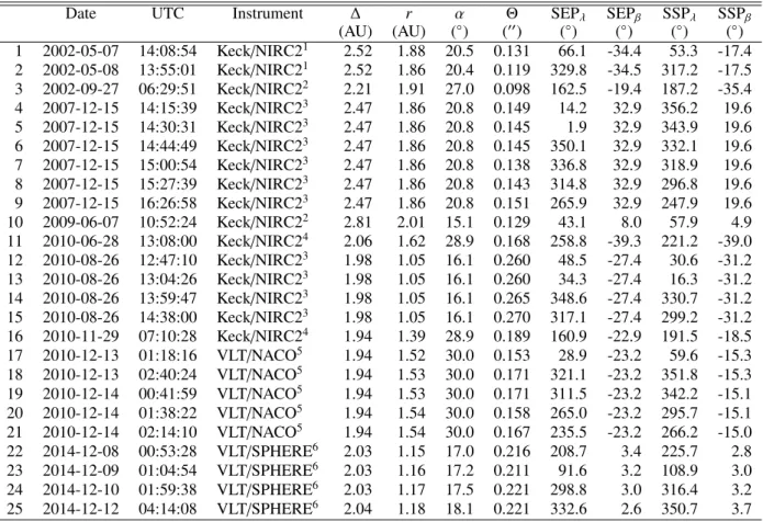
Two different models depicted in Fig.1were obtained; the first one using the light curves combined to the full AO sample, and the second one using the light curves and the SPHERE im-ages only. Comparison of the SPHERE-based model with our SPHERE images, earlier AO images, subsets of optical light curves and stellar occultations are presented in Figs.2,3,4, and

5, respectively.

The two models nicely fit all data, the RMS residuals be-tween the observations and the predictions by the model being only 0.6 pixels for the location of the asteroid contours, 0.02 magnitude for the light curves, and 5 km for the stellar occulta-tion of 2008 (the occultaocculta-tion of 1977 has very large uncertain-ties on its timings). The 3D shape models are close to an oblate spheroid, and have a volume-equivalent diameter of 196 ± 6 km (all AO) and 193 ± 6 km (SPHERE-based; Table2). Spin-vector coordinates (λ, β in ECJ2000) are close to earlier estimates based on light-curve inversion ((339◦_,+45◦_),_{Torppa et al.}_,₂₀₀₃_{) and} on a combination of light curves and AO images ((345◦_,+42◦_),

Hanuš et al.,2013).

The main difference between the two shape models comes from the presence of some surface features in the SPHERE-based model that are lacking in the model obtained using the full dataset of AO images. This is due to the lower resolution of earlier AO images that do not address some of the small-scale surface features revealed by the SPHERE images.

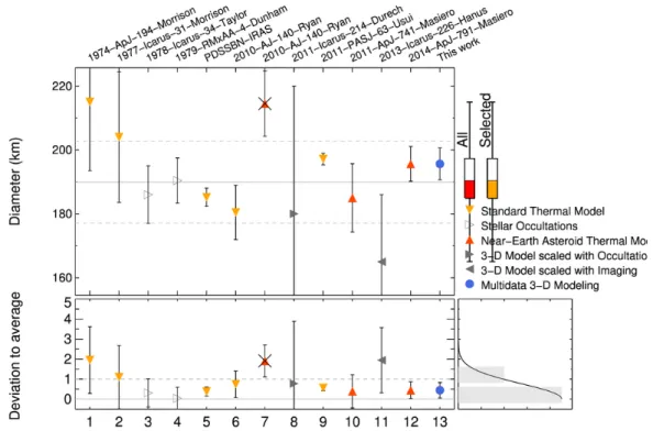
There are 12 diameter estimates for Hebe in the literature (TableA.1, FigureA.1). Rejecting values that do not fall within one standard deviation of the average value of the full dataset gives an average equivalent-volume sphere diameter of 191.5 ± 8.3 km, in very good agreement with the values of 193±6 km and 196 ± 6 km derived here (also supported by the thermophysical analysis presented in the following section). In the following,

Fig. 1.3D-shape model of (6) Hebe reconstructed from light curves and all resolved images (left), and from light curves and SPHERE images only (right). Viewing directions are two equator-on views rotated by 90◦

and a pole-on view.

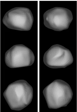
Fig. 2.Deconvolved SPHERE images of Hebe obtained between 8 and 12 December 2014 (top) and corresponding projection of the model (bottom). Orientation of the four images with respect to the North is 15.2◦_{, 12.8}◦_{, -5.3}◦_{and -89.6}◦_{, respectively.}

we use the value of the diameter obtained from our SPHERE-based model, which is more precise due to the higher angular resolution of the SPHERE images with respect to the NIRC2 and NACO images. A main advantage of using a diameter obtained from a full 3D shape modeling resides in the uncertainty on the derived volume V, which is close to δV/V ≈ δD/D, as opposed to a δV/V ≈ 3δD/D in the spherical assumption used in most aforementioned estimates (seeKaasalainen & Viikinkoski 2012

for details).

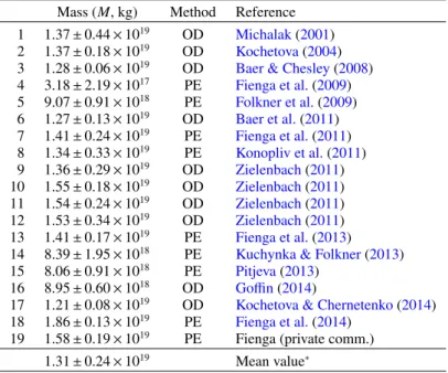
Combining this diameter with an average mass of 1.31 ± 0.24 × 1019 _{kg computed from 16 estimates gathered from the} literature (Table A.2, Figure A.2), provides a bulk density of 3.48 ± 0.64 g.cm−3_{, in perfect agreement with the average grain} density of ordinary H chondrites (3.42 ± 0.18 g.cm−3_;

Consol-magno et al. 2008). The derived density therefore suggests a null internal porosity, consistent with an intact internal ture. Hebe hence appears to reside in the volumetric and

(5)

struc-Article number, page 1 of1 Fig. 3.Previous AO images of Hebe obtained with Keck/NIRC2 and VLT/NACO (top of the three rows) and corresponding projection of the model (bottom). Each image is 0.8"×0.8" in size.

Rotation phase (7.274h period)

Relative flux 0.4 0.6 0.8 1.0 1.2 1 1959−02−05 α = 5.3o 129 points 6.95 h ADAM 0.01 Model RMS 2 1968−08−15 α = 20.6o 79 points 4.83 h ADAM 0.02 Model RMS 3 1971−05−15 α = 13.6o 89 points 5.96 h ADAM 0.03 Model RMS 4 1986−05−09 α = 14.3o 35 points 4.45 h ADAM 0.02 Model RMS 0.2 0.4 0.6 0.8 1.0 0.4 0.6 0.8 1.0 1.2 5 1991−08−18 α = 6.1o 92 points 7.95 h ADAM 0.02 Model RMS 0.2 0.4 0.6 0.8 1.0 6 2009−05−06 α = 7.9o 145 points 5.05 h ADAM 0.02 Model RMS 0.2 0.4 0.6 0.8 1.0 7 2012−03−01 α = 3.3o 82 points 7.64 h ADAM 0.01 Model RMS 0.2 0.4 0.6 0.8 1.0 8 2016−04−10 α = 10.7o 200 points 7.25 h ADAM 0.02 Model RMS

Fig. 4.Comparison of the synthetic light curves (solid line) from the shape model with a selection of light curves (gray points).

tural transitional region between the compact and gravity-shaped dwarf planets, and the medium-sized asteroids (∼10-100 km in diameter) with fractured interior (Carry,2012;Scheeres et al.,

2015). However, due to the current large mass uncertainty that dominates the uncertainty of the bulk density, the possibility of higher internal porosity cannot be ruled out. We expect the Gaia

Table 2.Period, spin (ECJ2000 longitude λ, latitude β and initial Julian date T0), and dimensions (volume-equivalent diameter D, volume V,

and tri-axial ellipsoid diameters a, b, c along principal axes of inertia) of Hebe derived with ADAM.

Parameter Value Value Unc. Unit

(all AO) (SPHERE-only)

Period 7.274467 7.274465 5.10−5 _hour λ 341.7 343.2 3 deg. β +49.9 +46.8 4 deg. T0 2434569.00 2434569.00 D 196 193 6 km V 3.95 ·106 _{3.75 ·10}6 _{1.2 ·10}5 _km3 a 218.4 213.4 6.0 km b 206.2 200.2 6.0 km c 172.1 172.6 6.0 km a/b 1.06 1.07 0.04 b/c 1.20 1.16 0.05

(6)

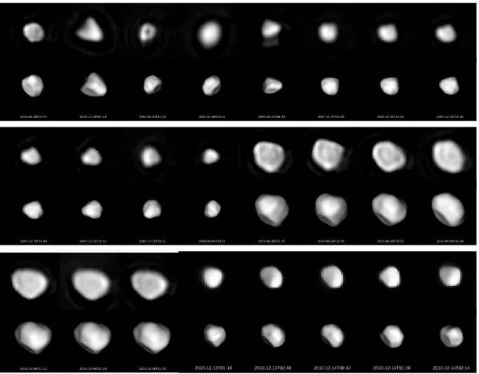
East−West (km)

North−south (km)

−200 −150 −100 −50 0 50 100 150 200 1 1977−03−05 02:34 2s CCD,Video Negative Visual Duration−only −150 −100 −50 0 50 100 150 200 250 300 350 400 −200 −150 −100 −50 0 50 100 150 200 2 2008−02−20 00:55 5s

Fig. 5.Comparison of the shape model with the chords from the occul-tation of 1977 and 2008.

future (Mignard et al.,2007;Mouret et al.,2007) that will help refine the density measurement of Hebe.

5. Thermal parameters and regolith grain size

A thermophysical model (TPM; Müller & Lagerros 1998;

Müller et al. 1999) was also used to provide an independent size measurement for Hebe and to derive its thermal surface proper-ties. The TPM uses as input our 3D shape model with unscaled diameter. The procedure is described in detail in AppendixB.

Using absolute magnitude H=5.71 and magnitude slope G=0.27 from the Asteroid Photometric Catalogue (Lagerkvist & Magnusson,2011), the TPM provides a solution for diam-eter and albedo of (D, pv)=(198+4−2km, 0.24±0.01), in good agreement with the size of our 3D-shape model and previous albedo measurements from IRAS (pv=0.27±0.01;Tedesco et al.

2002), WISE (pv=0.24±0.04;Masiero et al. 2014) and AKARI (pv=0.24 0.01;Usui et al. 2011). Best-fitting solutions are found for significant surface roughness (in agreement with Lagerros et al. 1999), and thermal inertia Γ values ranging from 15 to 90 J m−2_s−0.5_K−1_{, with a preference for}_{Γ ≈ 50 J m}−2_s−0.5_K−1_. Interestingly, we note that the best-fitting solution for Γ drops from ∼60 J m−2_s−0.5_K−1 _{when only considering thermal} mea-surements acquired at r<2.1 AU, to ∼40 J m−2_s−0.5_K−1_{for data} taken at r>2.6 AU. While this might be indicative of changing thermal inertia with temperature, this result should be taken with extreme caution, as the TPM probably overfits the data due to the large error bars on the thermal measurements (see AppendixB). From the thermal inertia value derived here, one can further derive the grain size of the surface regolith of Hebe (Gundlach & Blum,2013). Assuming values of heat capacity and material density typical of H5 ordinary chondrites (Opeil et al., 2010)

and estimated surface temperature of 230 K and 180 K at 1.94 and 2.87 AU respectively, we find that the typical grain size of Hebe is about 0.2–0.3 mm (see AnnexeBfor more details).

6. Topography

Hebe’s topography was investigated by generating an elevation map of its surface with respect to a volume-equivalent ellip-soid best-fitting our 3D-shape model, following the method by

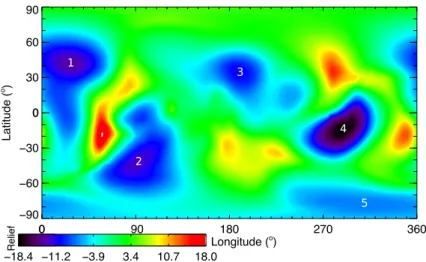
Thomas(1999). This map shown in Figure6allows the identifi-cation of several low-topographic and concave regions possibly created by impacts (the two shape models depicted in Fig.1 pro-duce slightly different but consistent topographic maps). Specif-ically, five large depressions (numbered 1 to 5 on the elevation map) are found at the surface of Hebe, at (29◦_{, 43}◦_{), (93}◦_, -42◦_{), (190}◦_{, 35}◦_{), (289}◦_{, -13}◦_{), and near the south pole.} Es-timated dimensions (diameter D and maximum depth below the average surface d) are D1=92–105 km, d1=13 km; D2=85– 117 km, d2=12 km; D3=68–83 km, d3=11 km; D4=75–127 km, d4=18 km; and D5=42–52 km, d5=7 km, respectively.

Assuming that the volume of a crater relates approximately to the volume of ejecta produced by the impact – which is most likely very optimistic because 1) a significant fraction of impact crater volume comes from compression (Melosh,1989) and, 2) at least a fraction of the ejecta must have re-accumulated on the surface of the body (e.g.,Marchi et al. 2015), one can further es-timate the volume of a hypothetical family derived from an im-pact on Hebe. The largest depression on Hebe roughly accounts for a volume of 105_km3_{, corresponding to a body with an} equiv-alent diameter of ∼58 km.

For comparison, the five known S-type families spec-trally analogous to Hebe (therefore to H chondrites; Ver-nazza et al. 2014) and located close to the main-belt 3:1 and 5:2 mean-motion resonances, namely Agnia (located at semi-major axis a=2.78 AU and eccentricity e=0.09), Koro-nis (a=2.87 AU, e=0.05), Maria (a=2.55 AU, e=0.06), Mas-salia (a=2.41 AU, e=0.14) and Merxia (a=2.75 AU, e=0.13) encompass a total volume of respectively ∼ 2.4 × 104 _km3_, 5.6 × 105 _km3_{, 3.6 × 10}5 _km3_{, 5.7 × 10}4 _km3 _{and 1.8 ×} 104 _km3 _{when the larger member of each family is} re-moved. Family membership was determined using Nesvorný

(2015)’s Hierarchical Clustering Method (HCM)-based classi-fication (http://sbn.psi.edu/pds/resource/nesvornyfam.html) and rejecting possible interlopers that do not fit the "V-shape" crite-rion as defined inNesvorný et al.(2015). The diameter of each asteroid identified as a family member was retrieved from the WISE/NEOWISE database (Masiero et al., 2011) when avail-able, or estimated from its absolute H magnitude otherwise, as-suming an albedo equal to that of the largest member of its family (respectively 0.152, 0.213, 0.282, 0.241 and 0.213 for (847) Agnia, (158) Koronis, (170) Maria, (20) Massalia and (808) Merxia;https://mp3c.oca.eu). We note that these values should be considered as lower limits as those families certainly include smaller members beyond the detection limit.

We therefore find that the volume of material correspond-ing to the largest depression on Hebe is of the order of some H-chondrite-like S-type families, and ∼4-6 times smaller than the largest ones. Therefore, although we cannot firmly exclude Hebe as the main (or unique) source of H chondrites, it appears that such a hypothesis is not the most likely one. This is further strengthened by the following two arguments. First, it seems im-probable that the volume excavated from Hebe’s largest depres-sion, which we find to be roughly 10 to 30 times smaller than the volume of the Rheasilvia basin on Vesta (Schenk et al.,2012b),

(7)

would contribute to ∼34% of the meteorite falls, when HED me-teorites only represent ∼6% of the falls (Hutchison,2004). We note, however, that the low number of HED meteorites may also relate to the relatively old age (Schenk et al.,2012b) of the Vesta family (Heck et al.,2017). Second, the current lack of obser-vational evidence for a Hebe-derived family indicates that such a family, if it ever existed, must be very ancient and dispersed. Yet, there is growing evidence from laboratory experiments that the current meteorite flux must be dominated by fragments from recent asteroid breakups (Heck et al.,2017). In the case of H chondrites, this is well supported by their cosmic ray exposure ages (Marti & Graf,1992;Eugster et al.,2006). It therefore ap-pears that a recent - yet to be identified - collision suffered by another H-chondrite-like asteroid is the most likely source of the vast majority of H chondrites.

7. Conclusion and outlook

We have reconstructed the spin and tridimensional shape of (6) Hebe from combined AO images and optical light curves, and checked the consistency of the derived model against avail-able stellar occultations and thermal measurements. Whereas the irregular shape of Hebe suggests it was moulded by impacts, its density appears indicative of a compact interior. Hebe thus seems to reside in the structural regime in transition between round-shaped dwarf planets round-shaped by gravity, and medium-sized aster-oids with fractured interiors (i.e., significant fractions of macro-porosity;Carry 2012). This however needs to be confirmed by future mass measurements (e.g., from Gaia high-precision astro-metric measurements) that will help improve the current mass uncertainty that dominates the uncertainty on density.

The high angular resolution of SPHERE further allowed us to identify several concave regions at the surface of Hebe possi-bly indicative of impact craters. We find the volume of the largest depression to be roughly five times smaller than the volume of the largest S-type H-chondrite-like families located close to or-bital resonances in the asteroid belt. Furthermore, this volume is more than an order of magnitude smaller than the volume of the Rheasilvia basin on Vesta (Schenk et al.,2012b) from which HED meteorites (∼6% of the falls) originate. Our results there-fore imply that (6) Hebe is not the most likely source of ordinary H chondrites (∼34% of the falls).

Finally, this work has demonstrated the potential of SPHERE to bring important constraints on the origin and collisional his-tory of the main asteroid belt. Over the next two years, our team will collect – via a large program on VLT/SPHERE (run ID: 199.C-0074, PI: Pierre Vernazza) – similar volume, shape, and topographic measurements for a significant number (∼40) of D≥100 km asteroids sampling the four major compositional classes (S, Ch/Cgh, B/C and P/D).

Acknowledgements. Based on observations made with ESO Telescopes at the La Silla Paranal Observatory under programme ID 60.A-9379. The asteroid diame-ters and albedos based on NEOWISE observations were obtained from the Plan-etary Data System (PDS). Some of the data presented herein were obtained at the W.M. Keck Observatory, which is operated as a scientific partnership among the California Institute of Technology, the University of California and the National Aeronautics and Space Administration. The Observatory was made possible by the generous financial support of the W.M. Keck Foundation. This research has made use of the Keck Observatory Archive (KOA), which is operated by the W. M. Keck Observatory and the NASA Exoplanet Science Institute (NExScI), under contract with the National Aeronautics and Space Administration. The au-thors wish to recognize and acknowledge the very significant cultural role and reverence that the summit of Mauna Kea has always had within the indigenous Hawaiian community. We are most fortunate to have the opportunity to conduct observations from this mountain. This research used the MP3_{C service}

devel-oped, maintained, and hosted at the Lagrange laboratory, Observatoire de la Côte

d’Azur (Delbo et al.,2017). Photometry of 6 Hebe was identified and extracted from WASP data with the help of Neil Parley (Open University, now IEA Read-ing). The WASP project is currently funded and operated by Warwick University and Keele University, and was originally set up by Queen’s University Belfast, the Universities of Keele, St. Andrews and Leicester, the Open University, the Isaac Newton Group, the Instituto de Astrofisica de Canarias, the South African Astronomical Observatory and by STFC. The WASP project is currently funded and operated by Warwick University and Keele University, and was originally set up by Queen’s University Belfast, the Universities of Keele, St. Andrews and Leicester, the Open University, the Isaac Newton Group, the Instituto de Astrofisica de Canarias, the South African Astronomical Observatory and by STFC. TRAPPIST-South is a project funded by the Belgian Funds (National) de la Recherche Scientifique (F.R.S.-FNRS) under grant FRFC 2.5.594.09.F, with the participation of the Swiss National Science Foundation (FNS/SNSF). E.J. and M.G. are F.R.S.-FNRS research associates. Based on observations with ISO, an ESA project with instruments funded by ESA Member States and with the participation of ISAS and NASA. Herschel is an ESA space observatory with science instruments provided by European-led Principal Investigator consortia and with important participation from NASA. Herschel fluxes of Hebe where extracted by Csaba Kiss (Konkoly Observatory, Research Centre for Astron-omy and Earth Sciences, Hungarian Academy of Sciences, H-1121 Budapest, Konkoly Thege Miklós út 15-17, Hungary). TM received funding from the Eu-ropean Union’s Horizon 2020 Research and Innovation Programme, under Grant Agreement no 687378.

References

Baer, J. & Chesley, S. R. 2008, Celestial Mechanics and Dynamical Astronomy, 100, 27

Baer, J., Chesley, S. R., & Matson, R. D. 2011, The Astronomical Journal, 141, 143

Belton, M. J. S., Chapman, C. R., Klaasen, K. P., et al. 1996, Icarus, 120, 1 Belton, M. J. S., Veverka, J., Thomas, P., et al. 1992, Science, 257, 1647 Berthier, J. 1999, Notes scientifique et techniques du Bureau des longitudes,

S064

Beuzit, J.-L., Feldt, M., Dohlen, K., et al. 2008, Ground-based Instrumentation for Astronomy, 7014, 701418

Binzel, R. P., Gaffey, M. J., Thomas, P. C., et al. 1997, Icarus, 128, 95 Binzel, R. P. & Xu, S. 1993, Science, 260, 186

Bottke, W., Vokrouhlický, D., Nesvorný, D., & Shrbeny, L. 2010, Bulletin of the American Astronomical Society, 42, 1051

Carry, B. 2012, Planetary and Space Science, 73, 98

Carry, B., Dumas, C., Fulchignoni, M., et al. 2008, Astronomy and Astrophysics, 478, 235

Carry, B., Dumas, C., Kaasalainen, M., et al. 2010a, Icarus, 205, 460

Carry, B., Kaasalainen, M., Leyrat, C., et al. 2010b, Astronomy and Astro-physics, 523, A94

Carry, B., Kaasalainen, M., Merline, W. J., et al. 2012, Planetary and Space Sci-ence, 66, 200

Consolmagno, G., Britt, D., & Macke, R. 2008, Chemie der Erde/ Geochemistry, 68, 1

Delbo, M., Tanga, P., Carry, B., Ordenovic, C., & Bottein, P. 2017, Asteroids, Comets, and Meteors: ACM 2017

Dunham, D. W., Herald, D., Frappa, E., et al. 2016, NASA Planetary Data Sys-tem, 243

Dunham, D. W. & Mallen, G. 1979, Revista Mexicana de Astronomia y As-trofisica, 4, 205

Durech, J., Kaasalainen, M., Herald, D., et al. 2011, Icarus, 214, 652

Durech, J., Sidorin, V., & Kaasalainen, M. 2010, Astronomy and Astrophysics, 513, A46

Eugster, O., Herzog, G. F., Marti, K., & Caffee, M. W. 2006, Meteorites and the Early Solar System II, 829

Farinella, P., Gonczi, R., Froeschle, C., & Froeschlé, C. 1993, Icarus, 101, 174 Fienga, A., Laskar, J., Kuchynka, P., et al. 2011, Celestial Mechanics and

Dy-namical Astronomy, 111, 363

Fienga, A., Laskar, J., Morley, T., et al. 2009, Astronomy and Astrophysics, 507, 1675

Fienga, A., Manche, H., Laskar, J., Gastineau, M., & Verma, A. 2013, eprint arXiv:1301.1510

Fienga, A., Manche, H., Laskar, J., Gastineau, M., & Verma, A. 2014, eprint arXiv:1405.0484

Folkner, W. M., Williams, J. G., & Boggs, D. H. 2009, Interplanetary Network Progress Report, 178, 1

Fujiwara, A., Kawaguchi, J., Yeomans, D. K., et al. 2006, Science, 312, 1330 Fusco, T., Mugnier, L. M., Conan, J.-M., et al. 2002, in Astronomical Telescopes

and Instrumentation, ed. P. L. Wizinowich & D. Bonaccini (SPIE), 1065 Fusco, T., Rousset, G., Sauvage, J. F., et al. 2006, Optics Express, 14, 7515

(8)

0 90 180 270 360 0 Longitude (o₎ −90 −60 −30 0 30 60 90 0 Latitude ( o) −18.4 −11.2 −3.9Relief 3.4 10.7 18.0 1 2 3 4 5

Fig. 6.Elevation map (in km) of (6) Hebe, with respect to a volume-equivalent ellipsoid best fitting our 3D-shape model. The five major depressions are identified by numbers.

Gaffey, M. J. & Fieber-Beyer, S. K. 2013, Meteoritics and Planetary Science Supplement, 76

Gaffey, M. J. & Gilbert, S. L. 1998, Meteoritics and Planetary Science, 33, 1281 Goffin, E. 2014, Astronomy and Astrophysics, 565, A56

Grice, J., Snodgrass, C., Green, S., Parley, N., & Carry, B. 2017, Asteroids, Comets, and Meteors: ACM 2017

Gundlach, B. & Blum, J. 2013, Icarus, 223, 479

Gwyn, S. D. J., Hill, N., & Kavelaars, J. J. 2012, Publications of the Astronomi-cal Society of the Pacific, 124, 579

Hanuš, J., Marchis, F., & Durech, J. 2013, Icarus, 226, 1045

Hanuš, J., Marchis, F., Viikinkoski, M., Yang, B., & Kaasalainen, M. 2017, As-tronomy and Astrophysics, 599, A36

Heck, P. R., Schmitz, B., Bottke, W. F., et al. 2017, Nature Astronomy, 1, 0035 Hutchison, R. 2004, Meteorites, ed. R. Hutchison

Jehin, E., Gillon, M., Queloz, D., et al. 2011, The Messenger, 145, 2 Kaasalainen, M. 2001, Icarus, 153, 37

Kaasalainen, M. & Torppa, J. 2001, Icarus, 153, 24

Kaasalainen, M. & Viikinkoski, M. 2012, Astronomy and Astrophysics, 543, A97

Kaasalainen, M., Viikinkoski, M., Carry, B., et al. 2011, EPSC-DPS Joint Meet-ing 2011, 416

Kochetova, O. M. 2004, Solar System Research, 38, 66

Kochetova, O. M. & Chernetenko, Y. A. 2014, Solar System Research, 48, 295 Konopliv, A. S., Asmar, S. W., Folkner, W. M., et al. 2011, Icarus, 211, 401 Kuchynka, P. & Folkner, W. M. 2013, Icarus, 222, 243

Lagerkvist, C. I. & Magnusson, P. 2011, NASA Planetary Data System, 162 Lagerros, J. S. V., Müller, T. G., Klaas, U., & Erikson, A. 1999, Icarus, 142, 454 Lenzen, R., Hartung, M., Brandner, W., et al. 2003, Ground-based

Instrumenta-tion for Astronomy, 4841, 944

Marchi, S., Chapman, C. R., Barnouin, O. S., Richardson, J. E., & Vincent, J. B. 2015, in Asteroids IV (University of Arizona Press)

Marti, K. & Graf, T. 1992, Annual Review of Earth and Planetary Sciences, 20, 221

Masiero, J. R., Grav, T., Mainzer, A. K., et al. 2014, The Astrophysical Journal, 791, 121

Masiero, J. R., Mainzer, A. K., Grav, T., et al. 2011, The Astrophysical Journal, 741, 68

Melosh, H. J. 1989, Research supported by NASA. New York, Oxford University Press (Oxford Monographs on Geology and Geophysics, No. 11), 1989, 253 p., 11

Merline, W. J., Drummond, J. D., Carry, B., et al. 2013, Icarus, 225, 794 Michalak, G. 2001, Astronomy and Astrophysics, 374, 703

Migliorini, F., Manara, A., Scaltriti, F., et al. 1997, Icarus, 128, 104

Mignard, F., Cellino, A., Muinonen, K., et al. 2007, Earth Moon and Planets, 101, 97

Morrison, D. 1974, The Astrophysical Journal, 194, 203 Morrison, D. 1977, Icarus, 31, 185

Mouret, S., Hestroffer, D., & Mignard, F. 2007, Astronomy and Astrophysics, 472, 1017

Mugnier, L. M., Fusco, T., & Conan, J.-M. 2004, Journal of the Optical Society of America A, 21, 1841

Müller, T. G. & Lagerros, J. S. V. 1998, Astronomy and Astrophysics, 338, 340 Müller, T. G., Lagerros, J. S. V., Burgdorf, M., et al. 1999, Asteroids, Comets,

and Meteors: ACM 2002, 427, 141

Nesvorný, D. 2015, NASA Planetary Data System, 234 Nesvorný, D., Brož, M., & Carruba, V. 2015, Asteroids IV, 297 Opeil, C. P., Consolmagno, G. J., & Britt, D. T. 2010, Icarus, 208, 449 O’Rourke, L., Müller, T., Valtchanov, I., et al. 2012, Planetary and Space

Sci-ence, 66, 192

Pavlov, A., Möller-Nilsson, O., Feldt, M., et al. 2008, Ground-based Instrumen-tation for Astronomy, 7019, 701939

Pitjeva, E. V. 2013, Solar System Research, 47, 386

Pollacco, D. L., Skillen, I., Collier Cameron, A., et al. 2006, Publications of the Astronomical Society of the Pacific, 118, 1407

Rousset, G., Lacombe, F., Puget, P., et al. 2003, Ground-based Instrumentation for Astronomy, 4839, 140

Russell, C. T., Raymond, C. A., Ammannito, E., et al. 2016, Science, 353, 1008 Russell, C. T., Raymond, C. A., Coradini, A., et al. 2012, Science, 336, 684 Ryan, E. L. & Woodward, C. E. 2010, The Astronomical Journal, 140, 933 Scheeres, D. J., Britt, D., Carry, B., & Holsapple, K. A. 2015, Asteroid Interiors

and Morphology, ed. P. Michel, F. E. DeMeo, & W. F. Bottke, 745–766 Schenk, P., O’Brien, D. P., Marchi, S., et al. 2012a, Science, 336, 694 Schenk, P., O’Brien, D. P., Marchi, S., et al. 2012b, Science, 336, 694 Sierks, H., Lamy, P., Barbieri, C., et al. 2011, Science, 334, 487

Tanga, P., Carry, B., Colas, F., et al. 2015, Monthly Notices of the Royal Astro-nomical Society, 448, 3382

Taylor, G. E. & Dunham, D. W. 1978, Icarus, 34, 89

Tedesco, E. F., Noah, P. V., Noah, M., & Price, S. D. 2002, The Astronomical Journal, 123, 1056

Tedesco, E. F., Noah, P. V., Noah, M., & Price, S. D. 2004, NASA Planetary Data System, 12

Thomas, P. 1999, Icarus, 142, 89

Thomas, P. C., Binzel, R. P., Gaffey, M. J., et al. 1997, Science, 277, 1492 Torppa, J., Kaasalainen, M., Michalowski, T., et al. 2003, Icarus, 164, 346 Usui, F., Kuroda, D., Müller, T. G., et al. 2011, Publications of the Astronomical

Society of Japan, 63, 1117

van Dam, M. A., Le Mignant, D., & Macintosh, B. A. 2004, Applied Optics, 43, 5458

Vernazza, P., Zanda, B., Binzel, R. P., et al. 2014, The Astrophysical Journal, 791, 120

Viikinkoski, M., Kaasalainen, M., & Durech, J. 2015a, Astronomy and Astro-physics, 576, A8

Viikinkoski, M., Kaasalainen, M., Durech, J., et al. 2015b, Astronomy and As-trophysics, 581, L3

Wizinowich, P. L., Acton, D. S., Lai, O., et al. 2000, Ground-based Instrumenta-tion for Astronomy, 4007, 2

Zielenbach, W. 2011, The Astronomical Journal, 142, 120

Zuber, M. T., Smith, D. E., Cheng, A. F., et al. 2000, Science, 289, 2097

Appendix A: Diameter and mass estimates from the literature

Diameter and mass estimates of (6) Hebe from the literature are presented here in TableA.1and FigureA.1 (diameter) and Ta-bleA.2and FigureA.2(mass). Average values were determined following the method byCarry(2012), which consists in reject-ing all the estimates that do not fall within one standard deviation of the average value, then by recomputing the average without these values.

(9)

Table A.1.Volume-equivalent diameter estimates of (6) Hebe gathered from the literature. STM: Standard Thermal Model, NEATM: Near-Earth Asteroid Thermal Model, LC: light curve, Occ: stellar occultation, AO: adaptative optics imaging, LC+Occ: light curve-based 3-D model scaled using an occultation, LC+AO: light curve-based 3D model scaled using adaptative optics images.

Diameter (D, km) Method Reference

1 215.00 ± 21.50 STM Morrison(1974)

2 201.00 ± 20.10 STM Morrison(1977)

3 186.00 ± 9.00 Occ Taylor & Dunham(1978)

4 190.40 ± 7.10 Occ Dunham & Mallen(1979)

5 185.18 ± 2.90 STM Tedesco et al.(2004)

6 180.42 ± 8.50 STM Ryan & Woodward(2010)

7 214.49 ± 10.25 NEATM Ryan & Woodward(2010)

8 180.00 ± 40.00 LC+Occ Durech et al.(2011)

10 197.14 ± 1.83 STM Usui et al.(2011)

11 185.00 ± 10.68 NEATM Masiero et al.(2011)

12 165.00 ± 21.00 LC+AO Hanuš et al.(2013)

13 195.64 ± 5.44 NEATM Masiero et al.(2014)

191.5 ± 8.3 Mean value∗

193 ± 6 ADAM (SPHERE only) This paper

196 ± 6 ADAM (all AO) This paper

198 ± 4/2 TPM This paper

Note:∗_{Using only values falling within 1-σ of the average value of the full dataset.}

Fig. A.1.Diameter estimates of (6) Hebe gathered from the literature.

Appendix B: Thermophysical model

The thermophysical model (TPM) used in this work predicts for a given set of parameters, including the volume-equivalent di-ameter D, albedo pv, surface roughness ¯θ, and thermal inertiaΓ, a flux that can be compared to the observed flux. The input pa-rameters can then be optimized by minimizing the reduced χ2 between the model and observations. Thermal measurements of Hebe used in the modeling procedure are plotted in FigureB.1.

Here, a solution was derived simultaneously forΓ, D and pv for a range of different ¯θ knowing Hebe’s absolute magnitude H and magnitude slope G. Different emissivity models,

includ-ing constant e=0.9 and wavelength-dependent emissivities, were tested. We adopted the emissivity model for large main-belt as-teroids ofMüller & Lagerros(1998) which was found to provide the most satisfactory results (lower χ2_{). Finally, best-fit solutions} were found for significant surface roughness andΓ values rang-ing from 20 to 100 J m−2_s−0.5_K−1 _(Figure_B.2_{). The resulting} observation-to-model flux ratios are shown at FigureB.3.

We further used a well established method (Gundlach & Blum,2013) to determine the grain size of the surface regolith of Hebe. The method consists in estimating the heat conductivity of the surface material derived from the thermal inertia

(10)

measure-Table A.2.Mass estimates of (6) Hebe gathered from the literature. OD: orbital deflection, PE: planetary ephemeris.

Mass (M, kg) Method Reference 1 1.37 ± 0.44 × 1019 _OD _Michalak₍₂₀₀₁₎

2 1.37 ± 0.18 × 1019 _OD _Kochetova₍₂₀₀₄₎

3 1.28 ± 0.06 × 1019 _OD _{Baer & Chesley}₍₂₀₀₈₎

4 3.18 ± 2.19 × 1017 _PE _{Fienga et al.}₍₂₀₀₉₎ 5 9.07 ± 0.91 × 1018 _PE _{Folkner et al.}₍₂₀₀₉₎ 6 1.27 ± 0.13 × 1019 _OD _{Baer et al.}₍₂₀₁₁₎ 7 1.41 ± 0.24 × 1019 _PE _{Fienga et al.}₍₂₀₁₁₎ 8 1.34 ± 0.33 × 1019 _PE _{Konopliv et al.}₍₂₀₁₁₎ 9 1.36 ± 0.29 × 1019 _OD _Zielenbach₍₂₀₁₁₎ 10 1.55 ± 0.18 × 1019 _OD _Zielenbach₍₂₀₁₁₎ 11 1.54 ± 0.24 × 1019 _OD _Zielenbach₍₂₀₁₁₎ 12 1.53 ± 0.34 × 1019 _OD _Zielenbach₍₂₀₁₁₎ 13 1.41 ± 0.17 × 1019 _PE _{Fienga et al.}₍₂₀₁₃₎

14 8.39 ± 1.95 × 1018 _PE _{Kuchynka & Folkner}₍₂₀₁₃₎

15 8.06 ± 0.91 × 1018 _PE _Pitjeva₍₂₀₁₃₎

16 8.95 ± 0.60 × 1018 _OD _Goffin₍₂₀₁₄₎

17 1.21 ± 0.08 × 1019 _OD _{Kochetova & Chernetenko}₍₂₀₁₄₎

18 1.86 ± 0.13 × 1019 _PE _{Fienga et al.}₍₂₀₁₄₎

19 1.58 ± 0.19 × 1019 _PE _{Fienga (private comm.)}

1.31 ± 0.24 × 1019 _{Mean value}∗

Note:∗_{Using only values falling within 1-σ of the average value of the full dataset.}

Fig. A.2.Mass estimates of (6) Hebe gathered from the literature.

ments and then to compare the values with calculations of the heat conductivity of a model regolith for distinct volume-filling factors of the regolith grains. The thermal inertia value and the surface temperature of these bodies are two input parameters for the method. First of all the thermal inertiaΓ is used to calculate the conductivity κ using:

κ = _φρcΓ2 , (B.1)

where c is the specific heat capacity, ρ the material density, and φ the regolith volume-filling factor, which is typically unknown. So, this last parameter is varied between 0.6 (close to the dens-est packing of equal-sized particles) and 0.1 (extremely fluffy packing, plausible only for small regolith particles) with∆φ=0.1, while here we take values for ρ and c typical of H5 ordinary chondrites fromOpeil et al.(2010). We estimate Hebe’s temper-ature to be 230 K and 180 K for the thermal inertia determination at 1.94 and 2.87 AU, respectively.

(11)

Fig. B.1.Thermal flux measurements of (6)-Hebe used for the ther-mophysical modeling. From IRAS (12, 25, 60, 100 µmTedesco et al. 2002), AKARI-IRC (9, 18 µmUsui et al. 2011), ISO-ISOPHOT (25 µm,

Lagerros et al. 1999), and Herschel-PACS (70, 100, 160 µm, Müller et

al., in prep).

Fig. B.2.Thermal inertia of (6) Hebe derived from the thermophys-ical modeling. The overall preferred solution (lower reduced χ2_{) is}

∼60 J m−2_s−0.5_K−1_{for data acquired at heliocentric distance r<2.1 AU}

and ∼40 J m−2_s−0.5_K−1_{for data taken at r>2.6 AU. While this might be}

indicative of changing thermal inertia with temperature, one should be extremely cautious when interpreting this result, as a range of solutions cannot be ruled out based on the χ2_{values presented here.}

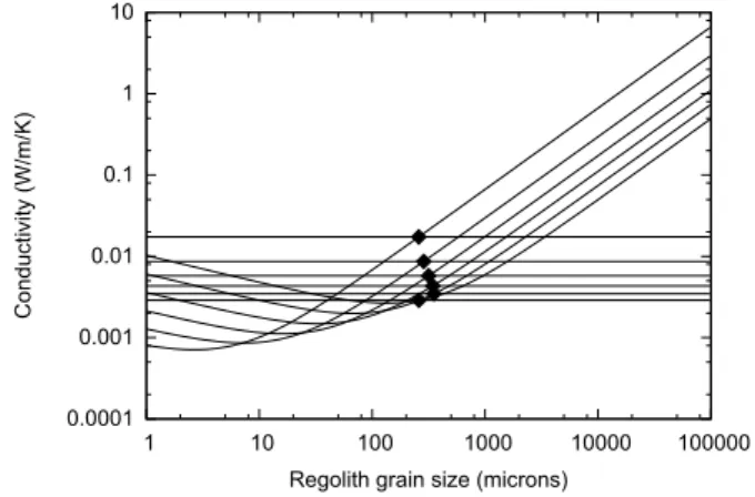
By doing so, we find a typical grain size of 0.2–0.3 mm (Fig-uresB.4andB.5).

Fig. B.3.Observation-to-model flux ratios as a function of wavelengths, based on color-corrected mono-chromatic flux densities and the corre-sponding TPM flux predictions.

0.0001 0.001 0.01 0.1 1 10 1 10 100 1000 10000 100000 Conduct ivit y (W /m/ K )

Regolith grain size (microns)

Fig. B.4.Hebe’s regolith grain size. Horizontal lines indicate the de-rived values of the heat conductivity, following Eq.B.1, for the different volume-filling factors of the material and for a thermal-inertia value of 40 J m−2_s−0.5_K−1_{and a surface temperature of 180 K. The curves}

rep-resent the thermal conductivity of a regolith with thermophysical prop-erties of a H5 meteorite as fromOpeil et al.(2010) as a function of the regolith grain size. The intersection of the curves with the horizontal lines gives the grain size of the regolith.

0.0001 0.001 0.01 0.1 1 10 1 10 100 1000 10000 100000 Conduct ivit y (W /m/ K )

Regolith grain size (microns)

Fig. B.5.Same as Fig.B.4but showing the regolith grain size for the a thermal inertia of 60 J m−2_s−0.5_K−1_{and a surface temperature of 230 K.}