This is an author-deposited version published in:
http://oatao.univ-toulouse.fr/
Eprints ID:5345
To link to this article
: DOI: 10.
1109/TSP.2011.2180718
http://dx.doi.org/10.1109/TSP.2011.2180718
To cite this version
:
Mittelman, Roni and Dobigeon, Nicolas and Hero,
Alfred O. Hyperspectral image unmixing using a multiresolution sticky
HDP. (2012) IEEE Transactions on Signal Processing, vol. 60 (n°4).
pp.1656-1671. ISSN 1053-587X
㩷O
pen
A
rchive
T
oulouse
A
rchive
O
uverte (
OATAO
)
OATAO is an open access repository that collects the work of Toulouse researchers and
makes it freely available over the web where possible.
Any correspondence concerning this service should be sent to the repository
administrator:
[email protected]
㩷Hyperspectral Image Unmixing Using a
Multiresolution Sticky HDP
Roni Mittelman, Member, IEEE, Nicolas Dobigeon, Member, IEEE, and Alfred O. Hero, III, Fellow, IEEE
Abstract—This paper is concerned with joint Bayesian
end-member extraction and linear unmixing of hyperspectral images using a spatial prior on the abundance vectors. We propose a gen-erative model for hyperspectral images in which the abundances are sampled from a Dirichlet distribution (DD) mixture model, whose parameters depend on a latent label process. The label process is then used to enforces a spatial prior which encourages adjacent pixels to have the same label. A Gibbs sampling frame-work is used to generate samples from the posterior distributions of the abundances and the parameters of the DD mixture model. The spatial prior that is used is a tree-structured sticky hierarchical
Dirichlet process (SHDP) and, when used to determine the
pos-terior endmember and abundance distributions, results in a new unmixing algorithm called spatially constrained unmixing (SCU). The directed Markov model facilitates the use of scale-recursive estimation algorithms, and is therefore more computationally efÞcient as compared to standard Markov random Þeld (MRF) models. Furthermore, the proposed SCU algorithm estimates the number of regions in the image in an unsupervised fashion. The effectiveness of the proposed SCU algorithm is illustrated using synthetic and real data.
Index Terms—Bayesian inference, hidden Markov trees,
hyper-spectral unmixing, image segmentation, spatially constrained un-mixing, sticky hierarchical Dirichlet process.
I. INTRODUCTION
H
YPERSPECTRAL imaging provides a means of iden-tifying natural and man-made materials from remotely sensed data [1], [2]. Typical hyperspectral imaging instruments acquire data in hundreds of different subbands for each spatial location in the image. Therefore each pixel is a sum of spectral responses of constituent materials in the pixel region, deÞned by the spatial resolution of the instrument.Spectral unmixing [3] is the process by which the hyperspec-tral data is deconvolved under a linear mixing model (LMM). In the LMM the observed spectrum in each pixel is described as a linear combination of the spectra of several materials (end-members) with associate proportions (abundances). A common
R. Mittelman and A. O. Hero III are with the Department of Electrical Engineering and Computer Science, University of Michigan, MI 48109 USA (e-mail:[email protected]; [email protected]).
N. Dobigeon is with the University of Toulouse, IRIT/INP-EN-SEEIHT/TéSA, BP 7122, 31071 Toulouse Cedex 7, France (e-mail:[email protected]).
solution to the unmixing problem is to use a two stage approach: endmember extraction followed by an inversion to compute the abundances. Two of the most popular endmember extraction al-gorithm are the N-FINDR [4] alal-gorithm, and vertex component analysis (VCA) [5]. However these methods assume the exis-tence of pure pixels in the observed image, i.e., they assume that for each of the materials there is at least one pixel where it is observed without being mixed with any of the other ma-terials. This assumption may be a serious limitation in highly mixed scenes. There have been several approaches presented in the literature to address the pure pixel assumption. In [6], a convex optimization based unmixing algorithm which uses a criterion that does not require the pure pixel assumption was presented. However the observation model assumes noise-free measurements and therefore the algorithm may not be effec-tive at low signal-to-noise ratio (SNR). A Bayesian linear un-mixing (BLU) approach which estimates the endmembers and abundances simultaneously and avoids the pure pixel assump-tion was presented in [7]. BLU also uses priors on the model variables which ensure endmember nonnegativity, abundance nonnegativity and sum-to-one constraints, and was shown to outperform the N-FINDR and VCA based unmixing algorithms for highly mixed scenes. Therefore, BLU can be considered as a state-of-the-art algorithm.
A common assumption underlying the aforementioned un-mixing algorithms is that the abundance vector for each pixel is independent of other pixels. When the spatial resolution (the size of the region that is represented by each pixel) is low it might be expected that neighboring pixels have different proportions of endmembers, however as the spatial resolution increases neighboring pixels are more likely to share similar spectral characteristics. Even low resolution images may have patches that are characterized by similar abundances, e.g., a large body of water or a vegetation Þeld. Including spatial constraints within the unmixing process has been receiving growing attention in the literature, and has been demonstrated to improve unmixing performance. In [8], spatially constrained unmixing was considered, however, the abundance nonneg-ativity and sum-to-one constraints as well as the endmember nonnegativity constraint were not enforced. The algorithms in [9] and [10] use spatial constraints to perform endmember extraction, however they rely on the pure pixel assumption. In [11] a spatially constrained abundance estimation algorithm that uses Markov random Þelds (MRF) [12] and satisÞes the abundance nonnegativity and sum-to-one constraints was pre-sented, however the endmembers were estimated separately without including any spatial constraints.
The MRF prior has been used extensively in domains such as texture [13] and hyperspectral [14], [15] image segmenta-tion. Although MRF based algorithms perform well they suffer
from several drawbacks. Inference in MRF is computationally expensive, and parameter estimation in the unsupervised setting is difÞcult [16]. Furthermore MRF estimation performance is highly sensitive to tuning parameters [17]. Although there exist methods such as the iterated conditional modes algorithm [18] that reduce the computational complexity related to inference in MRF, these methods usually only converge to a locally optimal solution, and limit the range of priors that may be employed in a Bayesian formulation. A common image processing alternative to MRF is the multiresolution Markov models deÞned on pyra-midally organized trees [19], which allow for computationally efÞcient scale-recursive inference algorithms to be used, and can be constrained to enforce local smoothness by increasing the self-transition probabilities in the Markov model.
In this paper, we develop a spatially constrained unmixing (SCU) algorithm that simultaneously segments the image into disparate abundance regions and performs unmixing. The abundances within each region are modeled as samples from a Dirichlet distribution (DD) mixture model with different parameters, thus the nonnegativity and sum-to-one physical constraints are naturally satisÞed. SpeciÞcally we use a mixture model with three components. The Þrst two mixture compo-nents capture the abundance homogeneity within the region by setting the precision parameter of the DD mixture components to be relatively large, and the third component models the outliers using a DD whose parameters are all set to one (this is equivalent to a uniform distribution over the feasibility set that satisÞes the nonnegativity and sum-to-one constraints). We avoid the need to deÞne the number of disparate homoge-neous abundance regions a priori by employing a hierarchical Dirichlet process (HDP) [20] type of prior. The standard HDP is a nonparametric prior in the sense that it allows the number of states in the Markov process to be learned from the data, and has been previously used for hidden Markov models and hidden Markov trees (HMT) [21], [22]. The multiresolution Markov model which we use differs from the hidden Markov models in [21] and [22] since the observations are only available at the bottommost level of the tree. To encourage the formation of spatially smooth regions we use the sticky HDP (SHDP) [23]. Our method has several advantages compared to the spatially constrained unmixing algorithms in [8]–[11]: (a) it is based on a directed multiresolution Markov model instead of a MRF and thus it allows the use of inference schemes which exhibit faster mixing rates; (b) the spatial dependencies are used to estimate both the abundances and the endmembers simultaneously, rather than just the abundances or endmembers; (c) it does not require the pure pixel assumption; (d) the number of regions that share the same abundances is inferred from the image in an unsupervised fashion. The SCU algorithm that we present here extends the work in [43] by modeling the abundance vectors in each cluster as samples from a DD mixture model with different parameters for each region, as opposed to Þxed abundances that are shared by all pixels within the region. Our experimental results show that in low SNR the spatial constraints implemented by the SCU algorithm signiÞcantly improves the unmixing performance.
This paper is organized as follows. Section II presents back-ground on the LMM for hyperspectral imaging, and the
abun-dance model. Section III presents the multiresolution prior and background on the SHDP. Section IV presents the spatially con-strained unmixing algorithm. Section V presents the experi-mental results, and Section VI concludes this paper.
II. PROBLEMFORMULATION
A. Hyperspectral Imaging With the LMM
A hyperspectral image is composed of pixels , where each is a -dimensional vector representing different spectral bands of the reßected electromagnetic Þeld. In the LMM each pixel measurement is a convex combination of
spectra vectors called endmembers,
corrupted by additive Gaussian noise
(1) where denotes the proportion of the material in the
pixel. The vector which is called
the abundance, must satisfy nonnegativity and sum-to-one con-straints
(2) We denote by the set of feasible abundances that satisfy the constraints (2). Similarly, since spectra are nonnegative, the endmember must satisfy
(3) Concatenating the vectors (1) into a matrix we have the equiv-alent matrix version of (1)
(4) where
(5) The objective of hyperspectral unmixing is to estimate the ma-trices and , given the observations .
B. Dimensionality Reduction
Due to the sum-to-one and nonnegativity constraints the abundance vectors lie on a simplex; a subspace of codimension 1. We use the principal component analysis (PCA) approach that was proposed in [7] to accomplish dimensionality reduc-tion. Let denote the mean vector of the columns of , and let denote the covariance matrix estimated using the columns of . Let denote a diagonal matrix with the largest eigenvalues of arranged along the diagonal, and similarly let denote a matrix with columns that are the appropriate eigenvectors, then the PCA reduced endmember takes the form (6)
where . Equivalently we have that
(7) where . The endmember matrix can therefore be expressed using as follows:
(8)
where .
The feasibility set for the endmember is expressed in terms of the PCA reduced representation as
(9)
where , , and is the
entry of .
C. The Dirichlet Distribution
The Dirichlet probability density function (PDF) with param-eter vector is [41]
(10) where . An alternative representation of the Dirichlet parameter vector is given by
(11) (12) where is the mean of the DD, and is known as the precision parameter.
The variance of the DD takes the form [41]
(13) and for we have that
(14) This implies that the DD PDF becomes more peaked around its mean as the precision parameter increases.
D. The Spatially Constrained Abundance Model
The unmixing algorithm that we present in this paper seg-ments the image into disparate regions. Let the different regions , denote disjoint sets composed of pixel in-dices, and let the indicator function of a pixel in region be deÞned as
if
otherwise (15)
The class label associated with pixel thus takes the form (16) The abundance of the pixel is generated using
(17)
where for , ,
, and we denoted , and
. The Þrst two mixture components capture the stial homogeneity of the abundances by setting the precision pa-rameter to a relatively large value, whereas the third component accounts for the outliers by setting to a relatively low value. The prior for the parameters , follows:
(18)
where , , and where
de-notes the uniform distribution on the interval and are parameters that satisfy . By setting to a relatively large value we can model the homogeneity of the abundances within a region. Furthermore we require
and in order for the likelihood function to be sufÞciently peaky and facilitate the estimation of the labels
. We Þxed the parameter values to ,
, , , , ,
throughout this work.
Let denote a discrete random variable which determines which mixture component was sampled from, then we can describe the generative model for the abundances using
(19) where the prior of is a multinomial probability mass function (PMF) of the form
(20) We also denote the sets and
for , .
In the sequel the labels , will be denoted since they are going to be associated with the maximal resolu-tion subset of a multiresoluresolu-tion tree in the SHDP representaresolu-tion described here.
E. Lower-Dimensional Abundance Representation
Since the abundances must satisfy the nonnegativity and sum-to-one constraints, they can be rewritten using the partial abundance vectors [7]
Fig. 1. A quadtree lattice.
and . The feasibility set is
(22)
III. THEMULTIRESOLUTIONSTICKYHDP
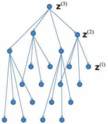
The LMM and the abundance model described in the previous section provide a statistical model for the observations, condi-tioned on the labels . To complete this model we also require a prior distribution for these labels, where in this paper we propose to use a multiresolution SHDP which can encourage the formation of spatially smooth label regions and determine the number of regions in an unsupervised fashion. Consider the quadtree lattice shown in Fig. 1, where the nodes are discrete random variables that take their values from the set , where denotes the number of class labels. We use the nota-tion , , to denote the labels at the level, where denotes the number of levels in the quadtree. We also deÞne the vector containing all the labels at the level
(23) The labels at the bottommost level of the quadtree are associated with the appropriate pixels of the hyperspectral image. We assume here that the number of pixels in the image is equal to the number of leaves at the bottommost level of the quadtree, otherwise one can increase the size of the tree and prune all the branches that have no descendants that correspond to image pixels. Our prior for the labels assumes a Markovian relationship between the labels on the quadtree lattice. SpeciÞ-cally, let us deÞne the likelihoods
(24) where denotes the parent of node at the level, then the joint probability mass function of all the labels takes the form
(25)
where , and . We also
deÞne the vector consisted of the transition probabilities from class label at the level
(26) The quadtree model can be used to enforce spatial smooth-ness by using a prior for ,
which encourages larger self-transition probabilities, i.e.,
, . Another issue is
the choice of the number of class labels . These type of problems are known as model order selection where common approaches such as the AIC [24] and BIC [25], optimize a criterion which advocates a compromise between the model Þtting accuracy and the model complexity. The drawback is that the AIC and BIC require a scoring function to be com-puted for every considered number of parameters in order to choose the optimal model. Another approach is reversible jump Markov chain Monte Carlo samplers [26], [27] where moves between different parameter spaces are allowed. However such methods require accurate tuning of the jump proposals and are not computationally efÞcient [28]. Dirichlet processes (DP) provide a nonparametric prior for the number of components in a mixture model [20] and facilitate inference using Monte Carlo or variational Bayes methods [29], [30]. The HDP is an extension of the DP which allows for several models to share the same mixture components, and can be used to infer the state space in a Markov model. The SHDP augments the HDP by encouraging the formation of larger self-transition probabilities in the Markov model, thus it provides an elegant solution to all the requirements of our multiresolution prior. Next we provide an introduction to the DP, HDP, and SHDP in the context of the tree prior which is used in the unmixing algorithm presented in this paper.
A. Dirichlet Processes
The DP denoted by is a probability distribution on a measurable space [31], and can be represented as an inÞnite mixture model where each component is drawn from the base measure , and the mixture weights are drawn from a stick-breaking process that is parameterized by positive real number [32]. SpeciÞcally, to sample from the DP one can sample the from the inÞnite mixture model
(27) where is the stick-breaking process constructed as fol-lows:
(28) (29) where denotes the Beta distribution. The stick-breaking process is commonly denoted by , and can be interpreted as dividing a unit length stick into segments that represent the proportions of the different mixture compo-nents . Observing (28) and (29), we note that setting such that is likely to be closer to one (i.e., smaller ) leads to having fewer mixing components with nonnegligible weights
and vice versa. Therefore the parameter expresses the prior belief on the effective number of mixture components. Equiva-lently, the generating process for a sample from , can be represented using an indicator random variable
(30) where denotes a multinomial distribution.
Another interpretation of the DP is through the metaphor-ical Chinese restaurant process (CRP) representation [20] which follows from the Pólya sequence sampling scheme [33]. According to the CRP, a customer that is represented by the sample index enters a restaurant with inÞnitely many tables each serving a dish . The customer can either sit at a new table where no one else is sitting, with probability that is proportional to , or sit at any other table with probability that is proportional to the number of other customers that are already sitting at that table. If the customer sits at a new table then he also chooses the dish served at that table by sampling the probability measure , otherwise the customer selects the dish that is served at the chosen table.
B. Hierarchical Dirichlet Processes
The HDP deÞnes a set of probability measures which are DPs that share the same base measure which is itself a DP. Let
, then the HDP is obtained using
(31) where denotes the number of different groups that share the same base measure , and is a positive real number. The process of generating a sample from can be repre-sented using the indicator variable notation
(32) Similarly to the DP, the HDP can be interpreted using a repre-sentation that is analogous to the CRP and is known as the Chi-nese restaurant franchise (CRF). The CRF metaphor describes each of the processes as restaurants that share the same global menu which offers dishes that are represented by the mixture components of . A customer that enters the restaurant can sit at an existing table with probability that is pro-portional to the number of other customers already sitting at that table, or at a new table with probability that is proportional to . If the customer sits at a table which is already instantiated he chooses the same dish that is served at that table, otherwise he chooses a dish by randomly drawing from . A dish which has already been served at any of the restaurants is sampled from with probability that is proportional to the number of all tables in the restaurants that are serving that dish, and a new dish is sampled from with probability that is proportional to .
Assuming a HDP prior, we can use in (32) as the transi-tion probabilities between the levels of the quadtree. The dishes correspond to samples from a base measure described by the
PDF of which can be obtained from (18), customers cor-respond to label realizations at the nodes of the quadtree, and the restaurant that each customer is assigned to corresponds to the label of the parent node, where we use different restaurants for each level in the tree.
C. The Sticky HDP
An important property that is demonstrated by the HDP is that the base measure serves as the “average” measure of all the
restaurants [23]
(33) The implication of (33) is that by using a HDP prior we as-sume that that the unique dish proportions are similar across dif-ferent restaurants. This violates our requirement that the prior for the transition probabilities encourage larger self-transition likelihoods. The SHDP [23] modiÞes the restaurant speciÞc dish likelihoods in (32) in the following manner:
(34) where is a nonnegative scalar, and denotes a vector with 1 at the entry and zeros in the rest. The “average” now takes the form
(35) and therefore the larger the parameter is, the more likely it becomes that the dish, which is referred to as the specialty dish, would be selected at the restaurant.
The metaphorical interpretation of the SHDP which is known as the CRF with loyal customers, is identical to the CRF with the sole difference that if a customer chooses to sit at an uninstan-tiated table at the restaurant, then in order to sample a dish he ßips a biased coin such that with probability proportional to
he selects the dish and with probability proportional to the customer draws the dish from . The table assignment of the sample at the restaurant thus follows:
(36) where denotes the number of customers sitting at the table in the restaurant, and denotes the number of tables instantiated in the restaurant. The dish assignment of a table in the restaurant is drawn using
(37) (38) (39) where denotes a Bernoulli distribution, , and is an auxiliary variable which is equal to zero or one, de-pending on whether the dish at the table in the restaurant
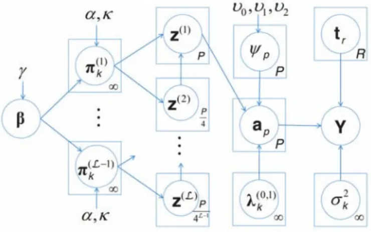
Fig. 2. Graphical model representation of the SCU algorithm, where is deÞned in (18), is deÞned in (20), is deÞned in (17), is deÞned in (6), is deÞned in (23), , is deÞned in (26), is the hyperspectral image, and is the variance of the observation noise in (4).
was chosen by drawing from , or by an override operation on the specialty dish.
1) InÞnite Limit of a Finite Mixture Model: The DP and the derived HDP and SHDP can all be obtained as the limit of Þ-nite mixture models [34], [35]. SpeciÞcally for the SHDP the stick-breaking process in (32) can be approximated as the
-dimensional DD
(40) and the restaurant speciÞc dish probabilities in (34) can be ap-proximated using the -dimensional DD
(41) The above construction converges in distribution to the SHDP
as .
2) Posterior Sampling in the SHDP: The approximation of the SHDP using Þnite mixture models leads to a simple form of the posterior distributions. By the conjugacy of the Dirichlet and multinomial distributions, it follows that:
(42)
where , which is also equivalent to
the number of customers that are having the dish in the restaurant. The posterior for takes the form
(43) where denotes the number of tables that are serving the dish all over the restaurants, which were not instantiated by an override operation of the specialty dish.
The posterior for the number of tables serving the dish in the restaurant in the SHDP takes the form [23]
(44)
where are unsigned Stirling numbers of the Þrst kind. Alternatively, it is possible to sample by simulating table assignments from a CRP [23].
The posterior for the override auxiliary variables given in (38) was developed in [23]:
(45) The number of tables whose dish was selected by sampling from satisÞes:
(46) where . A sample from the posterior for can be obtained using Algorithm 1.
Algorithm 1: Posterior sampling of
• For ,
1) Sample using (44) or by simulating from (36).
2) For , sample from (45).
3) Compute using (46).
IV. SPATIALLYCONSTRAINEDHYPERSPECTRALUNMIXING
WITH APYRAMIDSTRUCTUREDSHDP
In this section, we present the SCU algorithm where the graphical model representation is described in Fig. 2. We Þrst describe each of the parameters’ priors, and then present the posterior distributions that are used with the Gibbs sampling algorithm.
A. Parameter Priors
1) Label Transition Probabilities: The multiresolution Markov model described in Section III relies on the state
transition probabilities , , .
The prior for these parameters is obtained from the SHDP with the Þnite mixture approximation perspective. SpeciÞcally, we have that is a stick-breaking process that is ap-proximated using (40), and the prior for , , is obtained similarly to (41) with , regard-less of the value of .
2) Abundances: As described in Section II-D the abundance of pixel follows a DD mixture with a parameter vector which depends on the label
(47) where denotes the element of the vector .
3) DD Parameters: As explained in Section II-D, we use , where the priors for , and were de-scribed in Section II-D. Therefore
, . We assume that the parameters of the DD in every class are independent, therefore we have that
Algorithm 2: The SCU algorithm
• Initialization: initialize , , .
• Iterations: For
1) For , sample from (72).
2) Sample , using
(61).
3) For , , compute the
upward predictions using (58) and (60).
4) For , , sample the labels
using (56) and (57).
5) Partition all the labels into dishes and restaurants as described in Section IV-B.II.
6) Sample the number of tables serving the dish at the restaurant , using Algorithm 1 with
. 7) Sample from (43).
8) For , , sample
from (62).
9) For sample from (71).
10) For , sample as described in
Section IV-B.III.
11) For ,
— Sample using (67).
— For , sample using (65).
— For , set .
12) For , sample from (73). where denotes the abundance feasibility set (2).
4) The Indicator Variable : The prior for is given in (20), where as explained in Section II-D the parameters where chosen such that the prior promotes abun-dance PDFs which are peaky, and therefore facilitate the segmentation process.
5) Likelihood: We assume that the additive noise term in
the LMM satisÞes for all , thus the
likelihood of observing takes the form
(49)
where , and denotes the standard
Euclidean norm.
Since the noise vectors for each of the pixels , are assumed to be independent, the PDF of all the pixels takes the form
(50)
6) Noise Variance Prior: The prior which we use for is the conjugate prior
(51)
where denotes an inverse-gamma distribution, and we used the parameter values and .
7) Projected Spectra Prior: Similarly to [7] we use a multi-variate Gaussian that is truncated on the set given in (9), as a prior for . The PDF therefore takes the form
(52) where the mean is set using the endmembers found using VCA, and is set to a large value (we used ). B. Gibbs Sampling and the Posterior Distributions
The estimation is performed using a Gibbs sampler [36] which generates a Monte Carlo approximation of the distribu-tion of the random variables by generating samples from the posterior distributions iteratively, as outlined in Algorithm 2.
The posterior sampling schemes are described next in this section. Let , denote the sequence generated by the Gibbs sampler for a random variable , then the minimum mean squared error (MMSE) estimate is approximated using:
(53) where denotes the number of burn-in iterations.
A byproduct of the unmixing algorithm is the segmentation that is given by the labels . Since the random vector is discrete it can not be estimated like the abundances and endmembers using (53). One possible approach to segment the image is to select the which maximize the posterior likeli-hood, however this approach tends to overÞt the data [23]. The approach that we use in this work is known as the maximum of posterior marginals (MPM) [13], where the detected label for each pixel is that which occurs with the largest frequency over the sequence generated by the Gibbs sampler, i.e.
(54) 1) Block Sampling the Labels’ Posterior Distribution: The blocked sampler for the states of a HDP-HMT was presented in [22]. Here we present the particular case of the algorithm in [22] in which the observations are available at the leaf nodes alone, and which includes the SHDP extension of [23]. The approach is similar to the “upward-downward” procedure in hidden Markov trees [37]. The beneÞt of using a blocked sampler, as opposed to a direct assignment sampler which updates the label of a single node at a time, is that the mixing rate is improved signiÞcantly. A faster mixing rate translates into faster convergence.
The labels’ posterior can be written as
The interpretation of (55) is that given the appropriate condi-tional distributions, the block sampler is realized by sampling the labels at each level, going sequentially from the topmost level to the bottommost level. The conditional distributions in (55) admit the following expressions:
(56) (57) where in this paper we used an equally likely distribution for the labels . This choice ensures that the MCMC algorithm samples over the full depth of the tree. The upward predictions
are computed recursively using
(58)
where denotes the set consisted of the children of node at the level, and is obtained from (17). Equa-tion (58) therefore constitutes the upward sweep in which the predictions are calculated, whereas (56) implements a downward sweep in which the labels are sampled. Computing the integral in (58) is in general intractable, therefore we use Monte Carlo integration. Let denote the normalization con-stant of the truncated PDF , then we Þrst draw samples
(59) and approximate the integral using
(60) where in this paper we used . We note that in (60) can be ignored for the purpose of approximating (58), and the sam-pling in (59) can be realized by samsam-pling the partial abundance vector from a Gaussian PDF that is truncated to the partial abundance feasibility set
where
(61) We refer the reader to [7] for speciÞc details regarding the imple-mentation of efÞcient sampling from the truncated multivariate Gaussian distribution.
2) Posterior Sampling of the State Transition Probabilities: The labels effectively partition the data into restau-rants and dishes under the CRF with loyal customers metaphor. For instance assume that and , then as dis-cussed in Section III-B we interpret this as the dish being
served at the restaurant where . The pos-terior for is therefore obtained similarly to (42) using
(62) where . The posterior for is similarly given in (43).
3) Sampling From the Abundance Posterior: The abundance posterior at pixel takes the form
(63) with and given in (61).
The posterior for every element of is
(64) where denotes the length vector obtained by
ex-cluding from , , and are
the mean and variance of the Gaussian conditional PDF of given which can be obtained from (61) using [42, p. 324].
Sampling from the posterior for proceeds by evaluating (64) on a linearly spaced points in the interval , and sampling from the obtained PMF.
4) Sampling From the Posterior for : Instead of sam-pling from the posterior of directly, we sample from the posterior of and and set .
The posterior for takes the form
(65)
where , and denotes the cardinality
of the set . We sample from the posterior for by evalu-ating (65) on a linearly spaced points in the interval , and sampling from the obtained PMF.
Since the DD is in the exponential family it is easy to show that the posterior for is also in the exponential family, how-ever it does not have the form of any standard PDF. We therefore propose a different approach to approximately sample from the
posterior of . Let for , ,
then using (12) and the strong law of large numbers we have that
(66)
as . Therefore assuming that the number of samples is large the distribution of the sample mean
approx-Fig. 3. The ground truth abundance maps (a)-(e), and the true endmembers and the endmembers estimated using the VCA, SCU and BLU algorithms for SNR of 15 db (f)-(j). (a) endm. 1 abundance map. (b) endm. 2 abundance map. (c) endm. 3 abundance map. (d) endm. 4 abundance map. (e) endm. 5 abundance map. (f) endm. 1 spectra. (g) endm. 2 spectra. (h) endm. 3 spectra. (i) endm. 4 spectra. (j) endm. 5 spectra.
imates the distribution of the posterior. Using the central limit theorem to approximate the PDF of the sample mean we ap-proximate the posterior using
(67)
where
and where is a symmetric matrix with the diagonal elements and off diagonal elements for , which follows from (13) and (14). Since is unavail-able we replace it with the sample mean estimate . It can be seen that the approximate posterior distribution (67) converges to a Dirac delta function as the number of samples becomes larger. In order to enforce the nonnegativity and sum-to-one constraints for we replace the Gaussian PDF with a DD with the same mean and covariance matrix. Therefore we can sample approximately from the posterior of using
(69)
where .
5) Sampling the Posterior for : The posterior for is of the form
(70) where denotes the PDF of a DD for the random vector that is parameterized by . Similarly to (60) we use Monte Carlo integration to approximate the integral. We Þrst draw samples from (59), and then use the approximation
(71) where is a normalization constant which can be ignored. Therefore it is straightforward to sample by drawing from the normalized PMF (71). In this paper, we used .
6) Sampling From the Posterior for : The posterior for is an inverse Gamma distribution,
(72) 7) Sampling the Posterior for : The posterior for ,
is also multivariate Gaussian truncated to the feasi-bility set . Let denote the matrix with the column removed, then we have that
(73) where (74) with (75) C. Computational Complexity
The main additional complexity incurred by the use of the SHDP is due to the computation of the upward predictions in (58). For the complexity of (58) is , however
TABLE I
ABUNDANCEMEANS FOREACH OF THEREGIONS OF THESYNTHETIC
HYPERSPECTRALIMAGE
TABLE II
THE AND OF THEESTIMATEDENDMEMBERS FOR
DIFFERENTSNR
since the transition probabilities are very sparse it can ef-fectively be reduced to without any noticeable effect on the performance. The complexity of the proposed SCU algo-rithm is therefore dominated by the Monte Carlo approximation used in (58) for , which involves sampling from a trun-cated multivariate Gaussian. Let denote the complexity of sampling from a truncated multivariate Gaussian, then the com-plexity of SCU is approximately whereas the complexity of BLU is approximately since sampling the abundances entails the largest computational cost. Therefore the SCU runs about times slower than the BLU.
V. EXPERIMENTALRESULTS
A. Simulations With Synthetic Data
We generated a 100 100 synthetic hyperspectral image with 5 endmembers by simulating model (1) with , where the endmember spectra were taken from [38], and the abun-dances were sampled from a DD with precision parameter set to 60 and the means that are given in Table I. The synthetic abun-dance maps are shown in Fig. 3(a)–(e).
The ground truth and estimated endmembers for the 15 db scenario are shown in Fig. 3(f)–(j), where the SNR was deÞned as follows:
TABLE III
THESSEOF THEESTIMATEDABUNDANCES FORDIFFERENTSNR
Fig. 4. The segmentation obtained for SNR 15 db using the proposed SCU sticky HDP algorithm (a), and nonsticky SCU (b). (a) SCU. (b) Nonsticky SCU.
Fig. 5. A color visible band image corresponding to the hyperspectral image of Cuprite, NV. The region of interest is marked with the black frame.
where , , and .
The parameters that we used were , , and we used a truncation order of
to approximate the DPs. The number of levels in the quadtree
TABLE IV
THEMEAN, STANDARDDEVIATION, MINIMUM ANDMAXIMUM,
OBTAINEDUSING20 DIFFERENTINITIALIZATIONS FOR THEVCA, BLUAND
PROPOSEDSCU ALGORITHM FORDIFFERENTSNRS
Fig. 6. A satellite image of the region of interest obtained from Google Maps. The white lines represent roads.
was set to the maximum possible levels, where as described in Section III for a 100 100 image we Þrst extend the image to size 128 128 and prune all the branches that have no descen-dants that correspond to image pixels. The parameters , , and were estimated using the method described in [23]. However, we observed that the performance is not sensitive to the exact values of these parameters. The DD parameters were initialized by using the k-means algorithm to cluster the abundances (esti-mated using VCA) into classes, such that ,
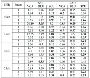
were set to the centers, and the precision parameters were set to , . In this paper, we assume that the number of endmembers is known, however, in practice the number can be estimated using model selection methods such as [40]. It can be seen in Fig. 3(f)–(j) that the spectra that was estimated using the proposed SCU algorithm is generally closer to the true endmembers compared to the endmembers extracted using the VCA abd BLU algorithms. Table II compares the sum of squared errors (SSE) and the spectral angle distance (SAD) for the VCA, BLU, and SCU for different SNR, where the SAD is deÞned as
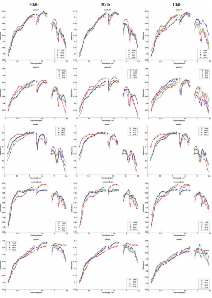
Fig. 7. The Þve estimated endmembers (Kaolin , Kaolin , Alunite , Montmorillonite , Sphene) for the proposed SCU algorithm as compared to ground truth and the VCA and BLU algorithms. SCU is competitive with the other methods at all SNRs.
It can be seen that the SCU performs comparably or better in all cases. The abundance SSE using the three methods is shown in
Table III, where it can be veriÞed that the SCU obtains lower SSE for almost all of the cases compared to the VCA and BLU.
TABLE V
THEMEAN, STANDARDDEVIATION, MINIMUM ANDMAXIMUM, OBTAINEDUSING20 DIFFERENTINITIALIZATIONS FOR THEVCA, BLU,
ANDPROPOSEDSCU ALGORITHM FORDIFFERENTSNRS
We did not observe signiÞcant differences in performance for this simulated example under different initializations and there-fore we do not report multiple random start statistics.
Fig. 4 shows the segmented images obtained using the pro-posed SCU algorithm when using the SHDP and the standard HDP. The SHDP identiÞed 9 classes with very few misclassi-Þed pixels whereas the HDP identimisclassi-Þed 38. Therefore, the SHDP more accurately identiÞed the underlying ground truth segmen-tation which had 9 classes. This demonstrates the signiÞcance of the stickiness property for segmentation purposes.
B. Simulations With Real AVIRIS Data
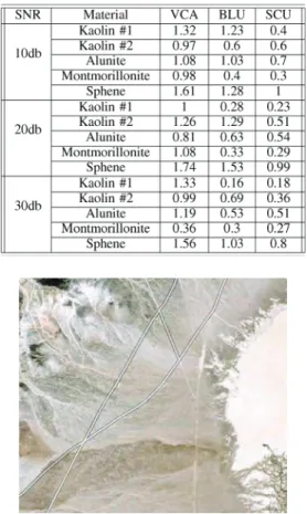
In this section, we test the new approach using the AVIRIS data of Cuprite, NV, [39] which has been used previously to demonstrate the performance of hyperspectral imaging algo-rithms [5], [7]. A color image synthesized from the hyperspec-tral image is shown in Fig. 5, where we used a 80 80 pixels region of interest which is marked with a black frame, to eval-uate the performance of the proposed SCU algorithm. Fig. 6 also shows a satellite image of the region of interest obtained from Google Maps, where the roads present in the image are marked by the white lines. The ground truth for the endmembers in this dataset is available at [38]. The parameter values and ini-tialization method that were used here were identical to those that were used for the synthetic image simulations, where we
used , and , and the
number of endmembers was set to 5. We ran the VCA, BLU, and SCU for 20 different times, where for each run we used the same endmember initialization obtained from the VCA algorithm for
the BLU and SCU algorithms. The SNR of the image as esti-mated by the VCA algorithm is about 30 db, therefore to illus-trate the beneÞts of the SCU algorithm in low SNR scenarios we also evaluated the performance when adding Gaussian noise to the hyperspectral image. Tables IV and V show the mean, stan-dard deviation, worst, and best SSE and SAD of the endmem-bers over the 20 runs, for SNRs of 10, 20, and 30 db. It can be seen that VCA estimates the Kaolin #1, Kailin #2, and Mon-tomorillonite endmembers quite well, which is most likely due to the existence of pure pixels in these materials for the scene under study. VCAÕs estimate of the Alunite and Sphene end-members is much worse, probably due to the lack of such pure pixels. Comparing the BLU and SCU it can be seen that on av-erage they perform comparably, however for the SCU the stan-dard deviation and worst case SSE is generally better than for the BLU. This shows that the SCU is more robust to the initial-ization of the endmembers in (52) which is obtained here using the VCA.
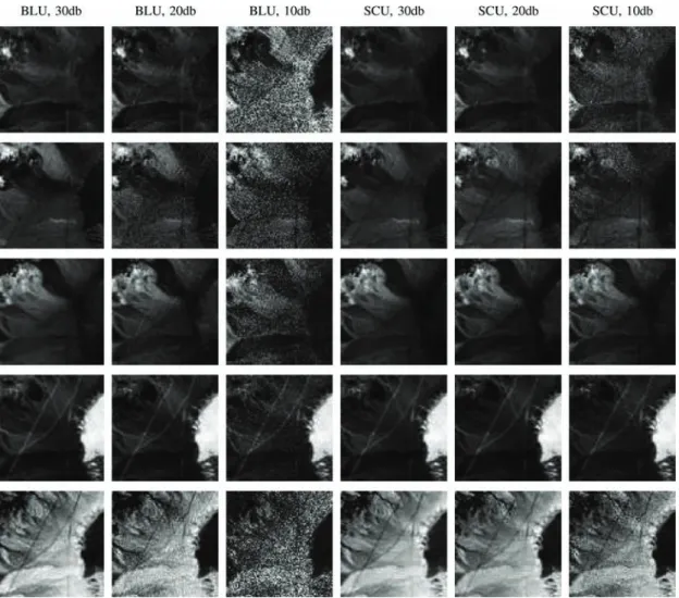
Figs. 7 and 8 show the estimated endmembers and the abundance maps, respectively, from one of the 20 runs for different SNR. It can be seen in Fig. 7 that the endmembers estimated using the BLU and SCU are generally comparable. Fig. 8 demonstrates that the abundance maps obtained using the SCU degrade far less as the SNR decreases compared to the abundances estimated using the BLU. Although we only show the results of one of the 20 runs, the abundance maps of the other runs look very similar to those shown in Fig. 8 thus it is representative of all our simulations.
There is no available ground truth for the abundances, how-ever we argue that since the roads that are present in the image and can be seen in Fig. 6 are man-made landmarks, the ground
Fig. 8. The estimated abundances. The algorithm and SNR for each column is written at the top row. Each row describe the abundances of the same material (from top to bottom: Kaolin #1, Kaolin #2, Alunite, Montmorillonite, Sphene).
TABLE VI
truth should demonstrate the property that the abundances along the roads are more similar to each other. Table V shows the variance of the variance of the road pixels abundances, where it can be seen that the variance of road pixels abundances is lower when using the SCU compared to the VCA and BLU. This suggests that the SCU estimates the abundances more accurately compared to the other algorithms.
VI. CONCLUSION
We presented a Bayesian algorithm, called the spatially con-strained unmixing (SCU) algorithm, which makes use of a spa-tial prior to unmix hyperspectral imagery. The spaspa-tial prior is en-forced using a multiresolution Markov model that uses a sticky hierarchical Dirichlet process (SHDP) to determine the number of appropriate segments in the image, where the abundances are sampled from Dirichlet distribution (DD) mixture models with different parameters. We take the spatial homogeneity of the abundances into accounted by including DD mixture compo-nents with large precision parameters, whereas the outliers are modeled using a mixture component that corresponds to a uni-form distribubution over the feasibility set which satisÞes the nonnegativity and sum-to-one constraints. Large regions with similar abundances are most likely to be found in high resolu-tion hyperspectral imagery, thus our proposed SCU approach is expected to be most beneÞcial in such images. However it is also useful in low resolution images that contain some large regions with similar abundances, e.g., a large body of water or a vegetation Þeld. The experimental results with synthetic and real data demonstrate that our proposed SCU algorithm has improved endmember and abundance estimation performance, particularly in low SNR regimes.
REFERENCES
[1] D. Landgrebe, “Hyperspectral image data analysis,” IEEE Signal
Process. Mag., vol. 19, no. 1, pp. 17–28, Jan. 2002.
[2] J. A. Richards, “Analysis of remotely sensed data: The formative decades and the future,” IEEE Trans. Geosci. Remote Sens., vol. 43, no. 3, pp. 422–432, Mar. 2005.
[3] N. Keshava and J. Mustard, “Spectral unmixing,” IEEE Signal Process.
Mag., vol. 19, no. 1, pp. 44–57, Jan. 2002.
[4] M. Winter, “Fast autonomous spectral end-member determination in hyperspectral data,” in Proc. 13th Int. Conf. on Appl. Geologic Remote
Sens., Vancouver, British Columbia, Apr. 1999, vol. 2, pp. 337–344.
[5] J. M. Nascimento and J. M. Bioucas-Dias, “Vertex component analysis: A fast algorithm to unmix hyperspectral data,” IEEE Trans. Geosci.
Remote Sens., vol. 43, no. 4, pp. 898–910, Apr. 2005.
[6] T. H. Chan, C. Y. Chi, Y. M. Hunag, and W. K. Ma, “A convex anal-ysis based minimum volume enclosing simplex algorithm for hyper-spectral unmixing,” IEEE Trans. Signal Process., vol. 57, no. 11, pp. 4418–4432, Nov. 2009.
[7] N. Dobigeon, S. Moussaoui, M. Coulon, J. Y. Tourneret, and A. O. Hero, “Joint Bayesian endmember extraction and linear unmixing for hyperspectral imagery,” IEEE Trans. Signal Process., vol. 57, no. 11, pp. 4355–4368, Nov. 2009.
[8] A. Plaza, P. Martinez, R. Perez, and J. Plaza, “Spatial/spectral end-member extraction by multidimensional morphological operations,”
IEEE Trans. Geosci. Remote Sens., vol. 40, no. 9, pp. 2025–2041, Sep.
2002.
[9] S. Jia and Y. Qian, “Spectral and spatial complexity-based hyperspec-tral unmixing,” IEEE Trans. Geosci. Remote Sens., vol. 45, no. 12, pp. 3867–3879, Dec. 2007.
[10] G. Martin and A. Plaza, “Spatial-spectral preprocessing for volume-based endmember extraction algorithms using unsuper-vised clustering,” in Proc. IEEE GRSS Workshop on Hyperspectral
Image and Signal Process: Evolution in Remote Sens. (WHISPERS),
Jun. 2010.
[11] O. Eches, N. Dobigeon, and J.-Y. Tourneret, “Enhancing hyperspec-tral image unmixing with spatial correlations,” IEEE Trans. Geosci.
Remote Sens., vol. 49, no. 11, pp. 4239–4247, Nov. 2011.
[12] J. Besag, “Spatial interaction and the statistical analysis of lattice sys-tems,” J. Royal Stat. Soc. Ser. B, vol. 36, no. 2, pp. 192–236, 1974. [13] M. L. Comer and E. J. Delp, “Segmentation of textured images using
a multiresolution Gaussian autoregressive model,” IEEE Trans. Image
Process., vol. 8, no. 3, pp. 408–420, Mar. 1999.
[14] G. Rellier, X. Descombes, F. Falzon, and J. M. Bioucas-Dias, “Tex-ture fea“Tex-ture analysis using Gauss Markov model in hyperspectral image classiÞcation,” IEEE Trans. Geosci. Remote Sens., vol. 42, no. 7, pp. 1543–1551, Jul. 2004.
[15] R. Neher and A. Srivastava, “A Bayesian MRF framework for labeling terrain using hyperspectral imaging,” IEEE Trans. Geosci. Remote
Sens., vol. 42, no. 7, pp. 1543–1551, Jul. 2004.
[16] C. A. Bouman, “A multiscale random Þeld model for Bayesian image segmentation,” IEEE Trans. Image Process., vol. 3, no. 2, pp. 162–177, Mar. 1994.
[17] N. Bali and A. M. Djafari, “Bayesian approach with hidden Markov modeling and mean Þeld approximation for hyperspectral data anal-ysis,” IEEE Trans. Image Process., vol. 17, no. 2, pp. 217–225, Feb. 2008.
[18] J. Besag, “On the statatistical analysis of dirty pictures,” J. Royal Stat.
Soc. Ser. B, vol. 48, no. 3, pp. 259–302, 1984.
[19] A. S. Willsky, “Multiresolution Markov models for signal and image processing,” IEEE Proc., vol. 90, no. 8, pp. 1396–1458, Aug. 2002. [20] Y. W. Teh, M. I. Jordan, M. J. Beal, and D. M. Blei, “Hierarchical
Dirichlet processes,” J. Amer. Statist. Assoc., vol. 101, no. 476, pp. 1566–1581, Dec. 2006.
[21] J. J. Kivinen, E. B. Sudderth, and M. I. Jordan, “Image denoising with nonparametric hidden Markov trees,” in Proc. IEEE Int. Conf. Image
Process. (ICIP), 2007.
[22] J. J. Kivinen, E. B. Sudderth, and M. I. Jordan, “Learning multiscale representations of natural scenes using Dirichlet processes,” in Proc.
IEEE Int. Conf. Comput. Vision (ICCV), 2007.
[23] E. B. Fox, E. B. Sudderth, M. I. Jordan, and A. S. Willsky, “The sticky HDP-HMM: Bayesian nonparametric hidden Markov models with per-sistent states,” MIT, Cambridge, MA, MIT LEADS Tech. Rep. P-2777, 2009.
[24] A. Hirotugu, “A new look at the statistical model identiÞcation,” IEEE
Trans. Autom. Contr., vol. 19, no. 6, pp. 716–723, Dec. 1974.
[25] S. Gideon, “Estimating the dimension of a model,” Ann. Statist., vol. 6, no. 2, pp. 461–464, 1978.
[26] P. J. Green, “Reversible jump MCMC computation and Bayesian de-termination,” Biometrika, vol. 82, pp. 711–732, 1995.
[27] C. Andrieu, P. M. Djuric, and A. Doucet, “Model Selection by MCMC Computation,” Signal Process., vol. 81, no. 1, pp. 19–37, Jan. 2001. [28] F. Bartolucci, L. Scaccia, and A. Mira, “EfÞcient Bayes factor
estima-tion from the reversible jump output,” Biometrika, vol. 92, no. 1, pp. 41–52, 2006.
[29] D. M. Blei and M. I. Jordan, “Variational inference for Dirichlet process mixtures,” Bayesian Anal., vol. 1, no. 1, pp. 121–144, 2005. [30] J. Paisley and L. Carin, “Hidden Markov Mmdels with stick-breaking
priors,” IEEE Trans. Signal Process., vol. 57, no. 10, pp. 3905–3917, Oct. 2009.
[31] T. S. Ferguson, “A Bayesian analysis of some nonparametric prob-lems,” Ann. Statistics, vol. 1, no. 2, pp. 209–230, Mar. 1973. [32] J. Sethuraman, “A constructive deÞnition of Dirichlet priors,”
Statis-tica Sinica, vol. 4, pp. 639–650, 1994.
[33] D. Blackwell and J. B. Macqueen, “Ferguson distributions via Pólya urn schemes,” Ann. Statist., vol. 1, no. 2, pp. 353–355, 1973. [34] H. Ishwaran and M. Zarepour, “Markov chain Monte Carlo
approxi-mate Dirichlet and beta two-parameter process hierarchical models,”
Biometrika, vol. 87, no. 2, pp. 371–390, 2000.
[35] H. Ishwaran and M. Zarepour, “Exact and approximate sum-represen-tations for the Dirichlet process,” Canadian J. Statist., vol. 30, no. 2, pp. 269–283, Jun. 2002.
[36] C. P. Robert and G. Casella, Monte Carlo Statistical Methods, 2nd ed. New York: Springer, 2004.
[37] M. Crouse, R. D. Nowak, and R. G. Baraniuk, “Wavelet – based sta-tistical signal processing using hidden Markov models,” IEEE Trans.
Signal Process., vol. 46, no. 4, pp. 886–902, Apr. 1998.
[38] R. N. Clark, G. A. Swayze, R. Wise, E. Livo, T. Hoefen, R. Kokaly, and S. J. Sutley, USGS Digital Spectral Library Splib06a, U.S. Geological Survey, 2007, vol. 231, Digital Data Series [Online]. Available: http:// speclab.cr.usgs.gov/spectral.lib06
[39] AVIRIS Free Data, Jet Propulsion Lab (JPL), Calif. Inst. Technol., Pasadena, CA, 2006 [Online]. Available: http://aviris.jpl.nasa.gov/ html/aviris.freedata.html
[40] N. Dobigeon, J. Y. Tourneret, and C. I. Chang, “Semi-supervised linear spectral unmixing using a hierarchical Bayesian model for hyperspectral imagery,” IEEE Trans. Signal Process., vol. 56, no. 7, pp. 2684–2695, Jul. 2008.
[41] T. P. Minka, Estimating a Dirichlet Distribution [Online]. Avail-able: http://research.microsoft.com/en-us/um/people/minka/papers/ dirichlet/minka-dirichlet.pdf
[42] S. M. Kay, Fundamentals of Statistical Signal Processing: Estimation
Theory. Englewood Cliffs, NJ: Prentice-Hall, 1993.
[43] R. Mittelman and A. O. Hero, “Hyperspectral image segmentation and unmixing using hidden Markov trees,” in Proc. IEEE Conf. on Image
Process. (ICIP), Hong Kong, Sep. 2010.
Roni Mittelman (S’08–M’09) received the B.Sc.
and M.Sc. (cum laude) degrees in electrical en-gineering from the Technion— Israel Institute of Technology, Haifa, and the Ph.D. degree in electrical engineering from Northeastern University, Boston, MA, in 2002, 2006, and 2009, respectively.
Since 2009, he has been a postdoctoral research fellow with the Department of Electrical Engineering and Computer Science, University of Michigan, Ann Arbor. His research interests include statistical signal processing, machine learning, and computer vision.
Nicolas Dobigeon (S’05–M’08) was born in
An-goulême, France, in 1981. He received the Eng. degree in electrical engineering from ENSEEIHT, Toulouse, France, and the M.Sc. degree in signal processing from the National Polytechnic Institute of Toulouse, both in 2004, and the Ph.D. degree in signal processing also from the National Polytechnic Institute of Toulouse in 2007.
From 2007 to 2008, he was a Postdoctoral Re-search Associate with the Department of Electrical Engineering and Computer Science, University of Michigan, Ann Arbor. Since 2008, he has been an Assistant Professor with the National Polytechnic Institute of Toulouse (ENSEEIHT – University of
Toulouse), within the Signal and Communication Group of the IRIT Labora-tory. His research interests are centered around statistical signal and image processing with a particular interest to Bayesian inference and Markov chain Monte Carlo (MCMC) methods.
Alfred O. Hero III (S’79–M’84–SM’96–F’98)
re-ceived the B.S. (summa cum laude) from Boston Uni-versity, Boston, MA, in 1980 and the Ph.D. degree from Princeton University, Princeton, NJ, in 1984, both in electrical engineering.
Since 1984, he has been with the University of Michigan, Ann Arbor, where he is the R. Jamison and Betty Williams Professor of Engineering. His primary appointment is with the Department of Electrical Engineering and Computer Science and he also has appointments, by courtesy, with the Department of Biomedical Engineering and the Department of Statistics. In 2008, he was awarded the Digiteo Chaire d’Excellence, sponsored by Digiteo Research Park in Paris, located at the Ecole Superieure d’Electricite, Gif-sur-Yvette, France. He has held other visiting positions at LIDS Massachu-setts Institute of Technology (2006), Boston University (2006), I3S University of Nice, Sophia-Antipolis, France (2001), Ecole Normale Supérieure de Lyon (1999), Ecole Nationale Supérieure des Télécommunications, Paris (1999), Lucent Bell Laboratories (1999), ScientiÞc Research Labs of the Ford Motor Company, Dearborn, Michigan (1993), Ecole Nationale Superieure des Tech-niques Avancees (ENSTA), Ecole Superieure d’Electricite, Paris (1990), and M.I.T. Lincoln Laboratory (1987–1989). His recent research interests have been in detection, classiÞcation, pattern analysis, and adaptive sampling for spatio-temporal data. Of particular interest are applications to network security, multimodal sensing and tracking, biomedical imaging, and genomic signal processing.
Dr. Hero was awarded a University of Michigan Distinguished Faculty Achievement Award in 2011. He has been plenary and keynote speaker at major workshops and conferences. He has received several best paper awards including: a IEEE Signal Processing Society Best Paper Award (1998), the Best Original Paper Award from the Journal of Flow Cytometry (2008), and the Best Magazine Paper Award from the IEEE Signal Processing Society (2010). He received the IEEE Signal Processing Society Meritorious Service Award (1998), the IEEE Third Millenium Medal (2000), and the IEEE Signal Processing Society Distinguished Lecturership (2002). He was President of the IEEE Signal Processing Society (2006–2007). He was on the Board of Directors of IEEE (2009–2011) where he served as Director Division IX (Signals and Applications).