Non-Uniform Time Sampling for Multiple-Frequency Harmonic Balance Computations

(1)

This is an author-deposited version published in:

http://oatao.univ-toulouse.fr/

Eprints ID: 8496

To link to this article: DOI: 10.1016/j.jcp.2012.11.010

URL:

http://dx.doi.org/10.1016/j.jcp.2012.11.010

To cite this version:

Guédeney, Thomas and Gomar, Adrien and Gallard,

François and Sicot, Frédéric and Dufour, Guillaume and Puigt, Guillaume

Non-Uniform Time Sampling for Multiple-Frequency Harmonic Balance

Computations. (2013) Journal of Computational Physics, vol. 236. pp. 317-345.

ISSN 0021-9991

Open Archive Toulouse Archive Ouverte (OATAO)

OATAO is an open access repository that collects the work of Toulouse researchers and

makes it freely available over the web where possible.

Any correspondence concerning this service should be sent to the repository

administrator:

staff-oatao@inp-toulouse.fr

(2)

Non-uniform time sampling for multiple-frequency harmonic

balance computations

Thomas Guédeney

a,b

_{, Adrien Gomar}

b,_⇑

_{, François Gallard}

b

_{, Frédéric Sicot}

b

_,

Guillaume Dufour

b,c

_{, Guillaume Puigt}

b

a_{Safran Snecma Villaroche, Rond-point René-Ravaud, 77550 Moissy-Cramayel, France}

b_{Centre Européen de Recherche et de Formation Avancée au Calcul Scientifique (CERFACS), CFD Team, 42 Avenue Gaspard Coriolis, 31057 Toulouse Cedex 1, France} c_{Université de Toulouse, Institut Supérieur de l’Aéronautique et de l’Espace (ISAE), 10 Avenue Edouard Belin, 31400 Toulouse, France}

a r t i c l e i n f o Keywords: Harmonic balance Almost-periodic flow Time sampling Condition number Turbomachinery a b s t r a c t

A time-domain harmonic balance method for the analysis of almost-periodic (multi-har-monics) flows is presented. This method relies on Fourier analysis to derive an efficient alternative to classical time marching schemes for such flows. It has recently received sig-nificant attention, especially in the turbomachinery field where the flow spectrum is essen-tially a combination of the blade passing frequencies. Up to now, harmonic balance methods have used a uniform time sampling of the period of interest, but in the case of sev-eral frequencies, non-necessarily multiple of each other, harmonic balance methods can face stability issues due to a bad condition number of the Fourier operator. Two algorithms are derived to find a non-uniform time sampling in order to minimize this condition num-ber. Their behavior is studied on a wide range of frequencies, and a model problem of a 1D flow with pulsating outlet pressure, which enables to prove their efficiency. Finally, the flow in a multi-stage axial compressor is analyzed with different frequency sets. It demon-strates the stability and robustness of the present non-uniform harmonic balance method regardless of the frequency set.

1. Introduction

The standard industrial design of multistage turbomachines is usually based on steady analysis, for which the most ad-vanced tools are three-dimensional Reynolds-Averaged Navier–Stokes (RANS) steady computations. With the ever growing need to improve performances, aggressive design choices foster unsteady phenomena, such as: blade interactions in com-pact turbo-engines, separated flows at/or close to stable operability limits, or aeroelastic phenomenon, to name but a few. In such a context, engineers now need tools to account for these effects as early as possible in the design cycle. With the growth of computational power, unsteady computations are entering industrial practice, but the associated restitution time remains an obstacle for daily basis applications. For this reason, efficient and/or accurate unsteady approaches are receiving a lot of attention. Different ways can be pursued to achieve an appropriate trade-off between efficiency and accuracy.

A first approach is to deal with the model equations: the Unsteady Reynolds-Averaged Navier–Stokes (U-RANS) equations can be simplified using some level of linearization (see Refs.[1–3]) to obtain a fast solution but with some limitations in

⇑Corresponding author.

E-mail addresses:thomas.guedeney@cerfacs.fr (T. Guédeney), adrien.gomar@cerfacs.fr(A. Gomar), francois.gallard@cerfacs.fr(F. Gallard), frederic. sicot@cerfacs.fr(F. Sicot),guillaume.dufour@isae.fr(G. Dufour),guillaume.puigt@cerfacs.fr(G. Puigt).

(3)

nonlinear regimes (see Ref.[4]for an example of accuracy issues, and Ref.[3]for some cure of stability problems). Con-versely, the Large-Eddy Simulation (LES) approach can be used to increase accuracy[5,6], but at a prohibitive cost.

A second approach, usually based on the U-RANS equations but not necessarily, is to work on the time-integration algo-rithm to reduce the computational cost as compared to standard time-marching techniques. To achieve this, Fourier-based methods for periodic flows have undergone major developments in the last decade (see He[7]for a recent review, or the special issue of the Int. J. CFD[8]). The basic idea is to decompose time-dependent flow variables into Fourier series, which are then injected into the equations of the problem. The time-domain problem is thus made equivalent to a frequency-domain problem, where the complex Fourier coefficients are the new unknowns. At this point, two strategies coexist to obtain the solution. The first one is to solve directly the Fourier coefficients, using a dedicated frequency-domain solver, as proposed by He and Ning[9,10]. The second strategy is to cast the problem back to the time domain using the inverse Fourier transform, as proposed by Hall [11,12] with the Harmonic Balance (HB) method. The unsteady time-marching problem is thus transformed into a set of steady equations coupled by a source term that is a high-order spectral evaluation of the time-derivative of the initial equations. The main advantage of solving in the time domain is that it can be imple-mented in an existing classical RANS solver, taking advantage of all classical convergence-accelerating techniques for steady state problems. The HB approach has demonstrated significant reduction of computational time, typically of a factor 2–10. In turbomachines, the relative motion of fixed and rotating blades gives rise to deterministic unsteady interactions at fre-quencies termed BPFs (Blade Passing Frefre-quencies). In a multi-stage turbomachine, a row sandwiched between two other rows is submitted to (at least) two BPFs (see Tyler and Sofrin[13]for instance), hence the need for multiple frequency meth-ods. Initially developed for single frequency problems, harmonic methods have been extended to account for multiple fre-quencies[14–16]. All the variations of the HB technique proposed in the literature rely on a uniform time sampling of the longest period of interest (though the number of samples can differ). Ekici and Hall[15]mention the use of non-uniform sampling but do not develop it. However, when the fundamental frequencies involved are significantly different, uniform sampling leads to an unnecessary high number of time samples: given that the shortest period has to be discretized by at least three instants (Shannon[17]requires at least two instants per period to capture a frequency, but an odd number of samples is required for stability issues[18]), uniform sampling of the longest period requires a total number of samples that grows with the largest to the shortest period ratio. This can compromise the efficiency of the method, as too many time sam-ples are computed. Besides, as demonstrated in the present contribution, uniform time sampling can also raise stability is-sues. To overcome these computational limitations, a new approach using non-uniform time sampling is proposed in the present contribution.

This paper is organized as follows: First, in Section2, mono- and multi-frequency HB methods are presented, and the im-pact of time sampling on numerical stability is discussed. Then, two algorithms for an automatic choice of the time samples are presented and compared in Section3. The proposed non-uniform sampling is assessed for a model problem in Section4. Finally, Section 5 is dedicated to the application to a turbomachinery configuration, with emphasis on the choice of frequencies.

2. Time-domain harmonic balance technique

The Unsteady Reynolds-Averaged Navier–Stokes (U-RANS) equations in integral form are given by Z X @W @t dV þ I @X ~_{F " ~}_{Nds ¼ 0;} _ð1Þ

where ~Fis the flux across @X and W is the vector of the conservative unknowns (conservative variables and turbulent vari-ables). Assuming X is a control volume, the semi-discrete finite-volume form of the U-RANS equations is obtained from Eq.(1):

d dt VW

! "

þ R W! "¼ 0; ð2Þ

with V the volume of the cell X; R the residual resulting from the discretization of the fluxes and the source terms (including the turbulent equations), and W the mean of the unknowns over the control volume. In the following, the over line symbol " is dropped out for clarity. Moreover, the mesh is considered not deformable, which allows to remove the volume V of the time derivative in Eq. (2), and simplifies explanations. However, the treatment remains valid if the mesh is deformable (see Ref.[4]for instance).

2.1. Periodic flows

V cWkþ bRk¼ 0; 8k 2 Z: ð5Þ

McMullen et al.[19–21]solve a subset of these equations up to mode N; &N 6 k 6 N, yielding the Non-Linear Frequency Domain (NLFD) method.

The principle of the time-domain harmonic balance approach, sometimes referred to as Time Spectral Method (TSM) [12,22], is to use an Inverse Discrete Fourier Transform (IDFT) to cast the equations back into the time domain. The IDFT then induces linear relations between Fourier coefficients cWkand a uniform sampling of W at 2N þ 1 instants in the period:

Wn¼

XN k¼&N

c

Wkexpði

x

nDtÞ; 0 6 n < 2N þ 1; ð6Þ

with Wn' WðnDtÞ and Dt ¼ T=ð2N þ 1Þ. This leads to a new system of 2N þ 1 mathematically steady equations coupled by a

source term:

RðWnÞ þ VDtðWnÞ ¼ 0; 0 6 n < 2N þ 1: ð7Þ

The source term VDtðWnÞ appears as a high-order formulation of the initial time derivative in Eq.(2). This new time operator

connects all the time levels and can be expressed analytically as DtðWnÞ ¼ XN m¼&N dmWnþm; ð8Þ with dm¼ p Tð&1Þmþ1csc 2Nþ1pm # $ ; m – 0; 0; _{m ¼ 0:} ( ð9Þ This equation clearly states that the source term is real for periodic flows. A similar derivation can be made for an even num-ber of instants, but it is proved in Ref.[18]that it can lead to a numerically unstable odd–even decoupling.

A pseudo-time ð

s

nÞ derivative is added to Eq.(7)to march the equations in pseudo-time to the steady-state solutions of all

the instants: V@Wn

@

s

n þ RðWnÞ þ VDtðWnÞ ¼ 0; 0 6 n < 2N þ 1: ð10Þ

This time step is defined locally in a given cell and can be different for all the HB instants. For stability reasons, its compu-tation is modified[18]to take into account the additional source term,

Dsn¼ CFL V

knnk þ

x

NV: ð11Þ

The extra term

x

NVis added to the spectral radius knnk to restrict the time step. Eq.(11)implies that a high frequency and/or

a high number of harmonics N can considerably restrict the time step, especially for explicit Runge–Kutta time integration scheme, as mentioned in[11]. Several implicit schemes, which are theoretically unconditionally stable and thus allow larger CFL number, have been derived for the HB method: Krylov-space based methods are used in[23,24], and Antheaume et al. [25] propose a point Jacobi algorithm. The present paper uses the block-Jacobi algorithm derived in Ref.[22]to improve robustness and efficiency.

This time-domain harmonic balance method has been implemented in the elsA solver[26] developed by ONERA and CERFACS. This code solves the RANS equations using a cell-centered approach on multi-blocks structured meshes. Using the HB method, significant savings in CPU cost have been observed in various applications such as dynamic derivatives com-putation[27], aeroelasticity[4]and rotor/stator interactions[28]. However, this approach is limited to periodic flows (i.e. a single fundamental frequency) and is unfit when the main frequencies of the system are not integers multiple of each other (such as multi-stage turbomachines for instance). The single-frequency HB method is therefore extended to the case where the flow is not periodic in time but is almost periodic.

(5)

2.2. Almost-periodic flows

2.2.1. Mapping on a set of arbitrary frequencies

If the flow variables are composed of non-harmonically related frequencies (i.e. the flow spectrum has high-energy discrete-frequency modes), the flow regime can be termed as almost-periodic[29]. Instead of a regular Fourier series, the U-RANS equations are projected on a set of complex exponentials with arbitrary angular frequencies

x

x

0t0Þ " " " expði

x

Nt0Þ

..

. _... _...

expði

x

&NtkÞ " " " expði

x

0tkÞ " " " expði

x

NtkÞ

x

N; . . . ;

x

0; . . . ;

x

NÞ; c WH ¼ ½cW&N; . . . ; cW0; . . . ; cWN*>; bRH ¼ ½bR&N; . . . ; bR0; . . . ; bRN*>: ð16Þ As opposed to the case of periodic flow, the arbitrary complex exponentials family does not form, a priori, an orthogonal basis.

Knowing a time sampling that allows A&1_{to be invertible, the almost-periodic Fourier coefficients can be approximated}

thanks to c WH ¼ AWH; with WH¼ Wðt½ 0Þ; . . . ; WðtiÞ; . . . ; W tð 2NÞ*>; bRH ¼ ARH; with RH¼ Rðt½ 0Þ; . . . ; RðtiÞ; . . . ; R tð2NÞ*>: ( ð17Þ Eq.(14)thus becomes

iVA&1_{PA þ R}H

¼ VDt½WH* þ RH¼ 0; ð18Þ

where the multiple-frequency HB time-derivative operator Dt½"* ¼ iA&1PA, the HB source term, can not be easily derived

ana-lytically, and has to be numerically computed. This must be real matrix, however the authors were not able to prove it math-ematically. Nonetheless, numerical experiments tends to confirm this assertion. Indeed, the magnitude of the ratio of the real part over the imaginary part is around 1015_{. The remaining value of the imaginary numbers may then be attributed to}

round-ing errors.

At this step of the derivation of the method, the time sampling ½t0; . . . ; t2N* remains to be specified.

2.2.2. Condition number and convergence

Kundert et al.[30]show that the condition number of A, and thus A&1_{, has a salient role in the convergence of harmonic}

In the case of periodic-flows, the DFT matrix is well-conditioned: the uniform sampling for harmonically related frequen-cies leads to a condition number equal to 1, which is the theoretical lower bound for the condition number. This is linked to the orthogonality of the complex exponential family. On the other hand, when the frequencies are arbitrary, it is usually impossible to choose a uniform set of time instants over which the almost-periodic DFT matrix A is well conditioned. In fact, it is common for uniformly-sampled sinusoids at two or more frequencies to be nearly linearly dependent, which causes them not to be orthogonal, leading to the ill-conditioning encountered in practice. As the frequency set is chosen by the user, the only degrees of freedom left to get a well-conditioned matrix are the time levels. The following section describes two algorithms to find a non-uniform time sampling that minimizes the almost-periodic DFT matrix condition number. 3. Non-uniform time sampling algorithms

Two algorithms that automatically choose the time levels in order to minimize the condition number are presented: first, the Almost Periodic Fourier Transform (APFT) algorithm, initially proposed in the literature for electronics problems, is de-scribed, then a gradient-based optimization algorithm over the condition number (OPT) is presented.

3.1. The APFT algorithm

Based on the work of Kundert et al.[30]in electronics, the APFT algorithm has been implemented. The aim of the APFT algorithm is to maximize the orthogonality of the almost-periodic DFT matrix in order to minimize its condition number. It is based on the Gram–Schmidt orthogonalization procedure. First, the greatest period 1=minkðfkÞ is oversampled with M

equally-spaced time levels, M + 2N þ 1 being specified by the user and N the number of frequencies. Considering these time levels, a rectangular almost-periodic IDFT matrix is built. Noting that every row of this matrix is a vector, a set of M vectors is obtained, numbered from 0 to M & 1, and of length 2N þ 1. The first vector V0(corresponding to t ¼ 0) is arbitrarily chosen as

the first time level and any component in the direction of V0is removed from the following vectors using the Gram–Schmidt

formula: Vs¼ Vs&V > 0 " Vs V> 0" V0 V0; s ¼ 1; . . . ; M & 1: ð22Þ

The remaining vectors are now orthogonal to V0. Since the vectors initially have the same Euclidean norm, the vector having

the largest norm is the most orthogonal to V0. It is assigned to V1. The previous operations are then performed on the M & 2

remaining vectors using V1as V0. This process is repeated until the required 2N þ 1 vectors are defined. As a time instant

corresponds to a vector, 2N þ 1 time levels are obtained, which enables the construction of the almost-periodic DFT matrix. This algorithm is summarized in Algorithm 1.

Algorithm 1. The almost periodic Fourier transform algorithm.

x

min min jð

x

kj; 1 6 k 6 NÞ for m 0; . . . ; M & 1 do tm _x2_minp m_M end for for n 1; . . . ; 2N do for m n þ 1; . . . ; M do Vm Vm&V_V>n>"Vm n"VnVn end for

argmax () returns the index of the largest member of a set k ¼ argmax kV! nsk; n þ 1 6 s 6 M"

swapðVnþ1; VkÞ

swapðtnþ1; tkÞ

end for

(7)

ðA T½ *Þ; Tini¼ TkÞ

3.3. Assessment of the algorithms

Let us consider the case of two frequencies, f1 and f. Without loss of generality it can be assumed that f6 f1. The

non-dimensional frequency d

(8)

d -f : ½0 : f1* # ½0 : 2* f # 2 "f1&f f1þf ( : ð25Þ

By taking f1constant, and having d-f sampled between 0 and 2, the whole range of f 6 f1is explored. Moreover, as d-f is

anti-symmetric ðd

ðAÞ is computed, highlighting the ability of

the different algorithms to choose the time levels that minimize the condition number, for any input frequencies. This assessment is only valid for two frequencies, but the tendency is similar when increasing the number of frequencies. Two frequencies are involved thus five time levels are required. The results of three algorithms are depicted inFig. 1: (i) APFT: the Almost Periodic Fourier Transform algorithm, (ii) OPT: the gradient-based optimization algorithm and (iii) EQUI: evenly spaced time levels oversampling the largest period as done in Gopinath et al.[14]using 2N þ 1 time levels and in Ekici and Hall[15,16]using 3N þ 1 time levels.

The EQUI algorithms give fair results ð

j

ðAÞ 6 2Þ only at discrete points, corresponding to the particular cases where f is a multiple of f1, which are thus similar to the single-frequency case. Oversampling improves the results. In fact, the mean

con-dition number obtained with 20N þ 1 time levels indicates that the higher the number of time levels the better the concon-dition number. However the almost-periodic DFT matrix becomes rectangular and the memory cost of such a computation in-creases drastically, preventing the use of such an approach on industrial cases. The APFT algorithm improves the results, as it gives results with

j

ðAÞ close to unity for 0:3 6 d

-f 6 1:2. However, when d-f tends to the boundaries (0 and 2), the

con-dition number seems to go to infinity. This corresponds to special values of f: d

-f ¼ 0 () f ¼ f1;

d

-f ¼ 2 () f ¼ 0: ð27Þ

This means that the APFT algorithm fails to work when the frequencies are too close to one another, and when they are sig-nificantly different. This limits the method for a range of frequencies where the HB method could give a salient gain in CPU time. Finally, the OPT algorithm gives a condition number close to unity for any value of d

-f. The OPT algorithm thus ensures

that the convergence of the HB method is not sensitive to the specified set of frequencies.Table 1summarizes the results obtained with each algorithm.

Table 1

Global results for the presented algorithms.

EQUI APFT OPT

# instants 2N þ 1 3N þ 1 20N þ 1 2N þ 1 2N þ 1

minðj½A*Þ 1:002 1:0 1:0 1:001 1:000

maxðj½A*Þ 3:024 , 1014 _{1:871 , 10}11 _2732:6 _823:8 _2:905

meanðj½A*Þ _{3:081 , 10}11 _{1:871 , 10}8 _10:92 _7:742 _1:097

(9)

Thus the proposed non-uniform time sampling combined with the OPT algorithm allows to tackle problems with large frequency separation. In such cases, the gain of the HB approach compared to classical time-marching methods is expected to be significant: with a time-marching scheme, the time-step has to be small enough to discretize the shortest period, while the number of time steps of the simulation has to be long enough to reach the (almost-) periodic state (i.e. the simulation time is equal to several times the longest period). Conversely, the cost of the HB method only depends on the number of frequencies to capture, regardless of their relative values.

3.4. Distribution of the time levels

For harmonically-related frequencies, the optimal time levels correspond to a uniform set sampling the fundamental fre-quency period as it gives the theoretical lower bound

j

ðAÞ ¼ 1. Since the frequencies are harmonically related, the distribu-tion of the time levels on the other frequencies is also uniform. Considering the frequency vector F ¼ ½f1; . . . ; fk¼ kf1; . . . ; Nf1*

and the time levels vector T: T¼ 0;_f 1 1" ð2N þ 1Þ; . . . ; 2N f1" ð2N þ 1Þ % & ; ð28Þ

then the product of the ith term of T to its associated frequency is f1"_f i 1" ð2N þ 1Þ¼ kf1" i kf1" ð2N þ 1Þ¼ fk" i fk" ð2N þ 1Þ: ð29Þ

Eq.(29)means that evenly-spaced time levels for the fundamental frequency are still seen as evenly spaced by the kth har-monic. This is an explanation why the condition number of the almost-periodic IDFT matrix A&1_{will be unity as each}

fre-quency is sampled by evenly spaced time levels[33].

Now, considering non-harmonically related frequencies, there is mathematically no reason for evenly-spaced time levels over the smallest frequency to be seen as evenly spaced by the other frequencies in general. Therefore, the use of non-evenly spaced time levels, and algorithms to automatically choose them, becomes necessary.

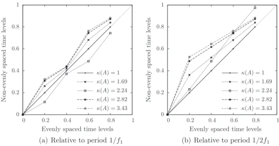
Fig. 2shows the distribution of the time levels, relative to each frequency period, obtained by the presented algorithms for the frequencies f1¼ 3 Hz and f2¼ 17 Hz (i.e. d-f ¼ 1:4). To do so, the chosen time levels are redistributed on the considered

frequency period by applying a modulo to it: T½fk*

j ¼ Tjmodulo1=fk: ð30Þ

Then, they are divided by the latter, so that the results are dimensionless. In light gray line is depicted the y ¼ x function representing the spaced solution on the considered period. Keeping in mind that if each frequency sees evenly-spaced time levels, then the condition number is the smallest, the optimal solution would be to have relative time levels on y ¼ x for each period. Running the EQUI, APFT and OPT algorithms leads to a condition number of 33.1, 3.8 and 1.1, respec-tively. The EQUI algorithm is perfect for the period 1=f1but is really far from the evenly spaced time levels for period 1=f2.

The APFT algorithm is far from the evenly spaced solution for both the periods considered, but closer than EQUI regarding period 1=f2. Finally, the OPT algorithm is the only one to be close to the evenly spaced solution for each considered period,

allowing the proposed HB method to be used for any set of frequencies.

(10)

The source code of the proposed algorithms and the scripts to generate inFigs. 1 and 2are available over the internet.1

The impact of the time sampling on HB computations is now investigated for the simple case of a channel flow with fluc-tuating pressure outlet.

4. Channel flow 4.1. Test case description

A channel configuration is set up to study the properties of the proposed HB method and the above algorithms for non-uniform time sampling. It is a 2D channel of length Lx¼ 100 m in the axial direction and Lz¼ 1 m in the transverse one. The

boundary conditions are: (i) an injection condition for the inlet, (ii) symmetric conditions for the upper and lower bounds as the flow is assumed to be symmetric in the transverse direction, and (iii) a fluctuating pressure imposed at the outlet:

PoutletðtÞ ¼ Pm" 1 þ A½ 1" sinð2

p

f1tÞ þ A2" sinð2

p

f2tÞ*; ð31Þ

where Pmis the temporal average static pressure, An the amplitude of the nth mode and fn its frequency. The mean outlet

pressure Pmis set to 60% of the inlet total pressure Pi0¼ 101; 325 Pa.

Pressure waves travel within the flow with the velocity u þ c and u & c, where u denotes the local flow velocity and c the sound velocity. Since the pressure waves are generated at the outlet, only the u & c waves are visible, resulting in pressure waves propagating upstream of the channel, which are damped by the effect of viscosity.Fig. 3shows a schematic diagram of the channel case, illustrating the propagation and attenuation of the pressure waves.

The mesh consists of 997 points along the axial direction and 9 in the transverse one, which amounts to almost equal spacings in both directions.

This configuration is turbulent as the Reynolds number based on the inlet flow velocity and the axial length of the channel is about Re( 2:0 , 109. Turbulence is modeled using the one-equation model of Spalart and Allmaras[34], and the

third-or-der upwind Roe scheme[35]is used to compute the convective fluxes. 4.2. Convergence sensibility analysis

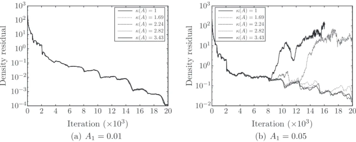
As mentioned previously, the condition number is of great importance for the convergence of the proposed HB method. To highlight this feature, the presented channel case is computed with a single frequency at the outlet: f1¼ 3 Hz with an

Fig. 3. Schematic diagram of the channel case.

Fig. 4. Distribution of the time levels on each frequency periods.

(11)

amplitude A1¼ 0:05 for the first case and A1¼ 0:01 for the second one, the second frequency having a zero amplitude:

A2¼ 0. Two frequencies are specified for the HB computation: f1 and its first harmonic 2f1. The time levels are chosen to

reach varying condition numbers such that 16

j

ðAÞ 6 3:43. Since the input frequencies of the HB computation are harmon-ically related, the minimal conditioning

j

ðAÞ ¼ 1 is obtained with evenly spaced time levels. The OPT algorithm is modified by subtracting the targeted conditioning to the objective function, so that the different condition numbers can be reached. The distribution of the time levels for each condition number is shown inFig. 4. The time levels deviate from the evenly spaced solution as the condition number grows. The results inFig. 5show that for a condition number

j

ðAÞ P 3:43 and wave input amplitude A1¼ 0:05, the computation diverges. However, the computations with the same condition numbers but a

smaller input amplitude A1¼ 0:01 converge. In fact, the condition number amplifies the errors made during the iterative

process. When the input waves have a smaller amplitude, the iterative errors are slighter, hence the convergence as ex-plained in Section2.2.2.

4.3. Validation of the multi-frequency HB method

To validate the proposed HB method, two non-harmonically related frequencies are chosen as input for the outlet bound-ary condition: f1¼ 3 Hz and f2¼ 17 Hz.

A classical time-marching scheme is taken for comparison, namely the Dual Time Stepping scheme (DTS[36]). The DTS method is a 2nd-order implicit time-marching scheme. Convergence in time discretization is obtained after 20 periods using 160 instants per almost-period. Since the frequencies are integers and coprime, the period is T ¼ 1 s. Iterative convergence

Fig. 5. Relation between the condition numberjðAÞ and the convergence of the solution.

(12)

for the inner loop is considered achieved when the normalized residuals drop by 10&2 _{within a maximum of 50}

sub-iterations.

The results obtained with the DTS scheme are compared to the HB results for pressure waves amplitudes of A ¼ A1¼ A2¼ 0:001. The transient of the DTS computation is shown inFig. 6, illustrating the wave propagation with a slight

attenuation of the high-frequency waves.

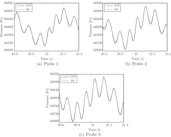
The results are analyzed for frequencies 1 < f < 40 Hz and the dominant frequencies (the one that have the highest amplitudes) are set for the HB computation. To do so, pressure signals are probed upstream, in the middle and downstream of the channel at x ¼ ½25 m;50 m;75 m* and z ¼ 0:5 m, respectively. The spectrum of the aforementioned unsteady pressure signals, obtained with a Fourier Transform, are plotted inFig. 7. The labeled frequencies are the dominant ones, as for each probe, these have a high amplitude. They are thus selected for the HB computation. For such frequencies, the OPT algorithm gives a set of time levels leading to a condition number of 1.4.

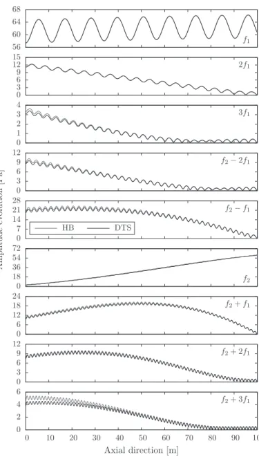
A Discrete Fourier Transform is computed at several axis positions, resulting in the spatial evolution of the different har-monics, which is used for the comparison of the HB and DTS approaches, in the middle of the canal ðz ¼ 0:5 mÞ. InFig. 8, the results are plotted for the frequencies that have been set for the HB computation. The overall agreement is fair. Some local discrepancies can be observed upstream for frequencies f2þ 3f1; f2& f1and f2& 2f1. These are caused by aliasing but they are

minimal regarding the temporal evolution, as shown inFig. 9, where the time evolution of pressure signals is extracted at all probes. The difference between the HB and the DTS method is negligible, proving that the proposed HB method is able to reproduce the unsteady almost-periodic phenomena.

The goal of this section was not to show significant CPU savings but rather the capacity of the present HB method to cap-ture an almost-periodic flow on a model problem. It is now applied to a more complex configuration, namely a turbomachin-ery element, where its computational efficiency is also emphasized.

5. Turbomachinery application

Under the assumption that all unsteady phenomena in a blade row during stable operation are periodic and can be cor-related with the rotation rate X of the shaft, the dominant frequencies are those created by the passage of the neighboring blades. In a multi-row turbomachine, a blade row sandwiched between the upstream and downstream rows is subjected to wake and potential effects. In practical turbomachines, the blade counts of neighboring rows are generally different and co-prime. Consequently, a sandwiched blade row resolves various combinations of the frequencies, which are additions and/or subtractions of multiples of the blade passing frequencies: according to Tyler and Sofrin[13], the kth frequency in the blade row j is given by

x

rowj k ¼ X nRows i¼1 nk;iBiðXi&XjÞ: ð32Þ

(13)

Here, Biand Xiare respectively the blade count and the rotation rate of the ith blade row, nk;iis the kth set of nRows integers

driving the frequency combinations. It must be noted that only the blade rows that are mobile relative to the considered j one contribute to its temporal frequencies and that every blade row solves its own set of frequencies and thus its own set of time levels. To set up a HB computation for a multistage configuration, it is of course impossible to use each and every pos-sible nk;i, and the user has to choose which frequency combinations will appear in the computation of each row.

In the literature, Gopinath et al. [14] and Ekici and Hall[15] assessed their implementation of the harmonic balance on a 2D multi-stage compressor (namely configuration D). It is composed of a rotor sandwiched by two stators having 32, 40 and 50 blades, respectively. Various combinations of the stators BPFs are considered, but always with evenly-spaced time levels sampling the largest period. While Gopinath et al. use 2N þ 1 samples, Ekici and Hall over-sample this period with 3N þ 1 time levels. This leads to a rectangular ð2N þ 1Þ , ð3N þ 1Þ almost-periodic Fourier Matrix and requires the computation of its Moore–Penrose pseudo-inverse. The chosen frequencies and the a posteriori associated condition numbers of the above references are given in Table 2. For N ¼ 4, the 3N þ 1 instants oversampling approach of Ekici and Hall efficiently reduces the condition number. But for this case, the use of evenly-spaced time levels is suf-ficient as the condition number seems to be small enough for the considered magnitude of unsteadiness. However, such an approach fails when dealing with more widely-separated frequencies as illustrated in the present contribution in Sec-tion3. Moreover, using an oversampling increases the CPU cost and the required memory as the number of steady com-putations to solve simultaneously is higher. These two reasons highlight the need for a non-uniform HB method as proposed in the current paper.

(14)

5.1. Boundary conditions for sector reduction

Section3showed how to contain the problem size by reducing the time span over which the solution is sought. In the following sections, it is explained how to cut down the mesh size by using a grid that spans only one blade passage per row. 5.1.1. Phase-lagged azimuthal boundary conditions

In a single blade passage computation of a multi-row configuration, the phase-lag condition[37]needs to be used to take the space–time periodicity into account. It states that the flow in one blade passage h is the same as next blade passage h þ Dh but at another time t þ dt:

Fig. 9. Unsteady pressure signals at different axial positions.

Table 2

Frequency combinations and associated condition number of computations made in the literature.

Frequencies jðAÞ

nS1 nS2 EQUI 2N þ 1 EQUI 3N þ 1 APFT OPT

N ¼ 2 1 0 3:79 3:00 1:72 1:08 Ref.[14] 0 1 1 0 N ¼ 3 0 1 5:40 3:84 1:71 1:00 Ref.[15] 1 1 1 0 N ¼ 4 0 1 11:25 2:07 3:46 1:13 Ref.[14] 1 1 1 &1 1 0 0 1 1 1 N ¼ 7 1 &1 16:66 14:61 12:95 1:00 Ref.[14] 2 0 2 &1 2 1

(15)

W h þð Dh; tÞ ¼ W h; t þ dtð Þ; ð33Þ where Dh is the pitch of the considered row. Assuming that every temporal lag is associated with a rotating wave of rota-tional speed

x

k, the constant time lag can be expressed as

dt ¼

_x

bk k; 8k; ð34Þ where bk¼ 2

p

signð

x

kÞ 1 &_B1 j X i–j nk;iBi ! ; ð35Þ

the nk;ibeing the integers specified for the computation of the frequencies from Eq.(32), Bithe number of blades in row i and

subscript j denoting the current row.

The phase-lag condition was adapted to the time-domain HB by Gopinath et al.[12]. The derivation starts with the al-most-periodic Fourier transform of Eq.(33):

XN k¼&N c Wkðh þDh; tÞeixkt¼ XN k¼&N c Wkðh; tÞeixkdteixkt: ð36Þ

Thus, the flow spectrum from one blade passage is equal to that of the next blade passage modulated by the inter-blade phase angle bk:

c

Wkðh þDh; tÞ ¼ cWkðh; tÞeixkdt¼ cWkðh; tÞeibk: ð37Þ

Using the same notation as previously, the following matrix formulation is obtained: WH

¼ A&1MAWHðhÞ; ð38Þ

where

M ¼ diagð&bN; . . . ;b0; . . . ;bNÞ; ð39Þ

and A&1_{is given by Eq.}₍₁₅₎_.

5.1.2. Stage coupling

Each blade row has its own frequency set and therefore its own time sampling. Therefore, the nth time level in the jth and ðj þ 1Þth rows do not necessarily match the same physical time. Consequently, at the interface between adjacent blade rows, the flow field on the donor side needs to be generated for all the time levels of the receiver side using a spectral interpolation. A non-abutting join interface is used to perform the spatial communications between the two rows[38]. In order to account for the pitch difference and relative motion, a duplication of the flow is carried out in the azimuthal direction using the phase-lag periodicity. Moreover, as described in Ref.[28], the time levels at the interface are oversampled and filtered to pre-vent aliasing.

5.2. Application to a subsonic compressor

In order to validate the non-uniform HB method on a turbomachinery test case, a subsonic compressor case is studied. It is the mid-span slice of the inlet guide vanes (IGV) and the first stage of the axial compressor CREATE[39], located in Lyon

(16)

(France) at the Laboratoire de Mécanique des Fluides et Acoustique (LMFA). This configuration is composed of 32 IGV blades, 64 rotor (RM1) blades and 96 stator (RD1) blades. The full 3D 3.5-stage computation is presented in Ref.[40].

5.2.1. Mesh and numerical parameters

As shown inFig. 10, the blade passages are meshed with a block-structured topology. It is composed of five grid points in the radial direction, 33 in the azimuthal direction and 100 in the axial direction for both rows. This leads to a total number of approximately 50,000 mesh cells.

The IGV blade is not actually meshed but taken into account through a non-uniform injection boundary condition that represents the wake of the IGV entering the RM1 domain. This injection follows the self-similarity law of Lakshminarayana and Davino[41], which states that the spatial evolution of a wake can be described by a Gaussian function. As BRD1¼ 3 " BIGV,

the frequency content remains mono-frequential in the rotor (i.e., the BPF of the downstream rotor is just an harmonic of the Fig. 11. Valve condition at the outlet.

(17)

IGV’s BPF). Therefore the number of blades composing the IGV has been changed from 32 to 80 so that the configuration still presents a 2

p

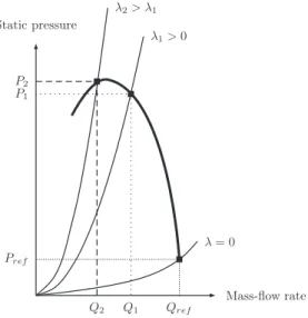
=16 periodicity but the frequency content is now multi-frequential in the rotor.

The outlet duct is modeled by a valve condition coupled with a simplified radial equilibrium equation. The reference out-let static pressure Psfor the radial equilibrium integration is imposed according to the formula Ps¼ Prefþ kðQ=QrefÞ2, as

illus-trated inFig. 11. Pref is a reference static pressure chosen such that when k ¼ 0 Pa the compressor is choked, and Qref is the

corresponding mass flow. Q is the current mass flow and k P 0 is a user-defined pressure. Its different values allow to move along the compressor map: when k increases, the outlet static pressure rises and the mass flow rate decreases and vice versa (Fig. 11). At the blades’ surfaces, wall laws[42]are imposed. The lower and upper radial conditions are slip walls.

The convective fluxes are discretized using the second-order Jameson scheme[43]with added artificial viscosity, or a sec-ond-order Roe scheme[35,44]. For this study, the turbulent viscosity is computed with the one-equation model proposed by Spalart and Allmaras[34].

The DTS scheme is used to get a numerical reference solution. The periodicity of the different blade passages is such that a 2

p

=16 periodicity is enough to perform the unsteady computations. To reach an established periodic state, 67 passages (using 400 instants per azimuthal period) of the periodic sector are necessary.

Fig. 12plots the time evolution of the fluid density

q

and its associated spectrum downstream of the rotor. The spectrum is not only composed of the blade passing frequencies and their harmonics but also of combinations of them as estimated by Tyler and Sofrin[13]. The amplitude of a frequency combination may also be higher than an harmonic of a blade passing frequency. For example, BPFIGV& BPFRD1is higher than the third and fourth harmonics of BPFRD1. This highlights the necessity

of being able to take into account these frequency combinations in a HB computation. 5.2.2. A posteriori computations: HB computations with frequencies known beforehand

5.2.2.1. Frequency content, time sampling and convergence. The convergence of the harmonic balance computations is done in two steps: first 15,000 iterations with a second order Roe scheme, then 10,000 iterations with the Jameson scheme (with the Table 3

Frequency combination coefficients.

nIGV nRM1 nRD1 Initialization

1 1 &1 Restart from steady computation

N ¼ 3 1 2 0 15,000 it. with Roe second order scheme

0 3 1 then 10,000 it. with Jameson scheme

jðAÞ APFT 1.0 2.0 1.0

N ¼ 4 v1 1 2 0 15,000 it. with Roe second order scheme

1 4 1

jðAÞ APFT 1.0 1.0 1.0

2 4 0

jðAÞ APFT 1.0 1.76 1.0

0 4 2

jðAÞ APFT 1.0 2.0 1.0

1 1 &1

1 2 0 Restart from N ¼ 4 v1

N ¼ 5 0 3 1 10,000 it. with Jameson scheme k4¼ 0:064

2 4 0 then 10,000 it. with Jameson scheme k4¼ 0:032

0 5 2

jðAÞ APFT 1.0 2.34 1.0

1 1 &1

2 2 &2 Restart from N ¼ 5

N ¼ 6 1 3 0 5000 it. with Jameson scheme k4¼ 0:064

0 4 1 then 5000 it. with Jameson scheme k4¼ 0:032

2 5 0

0 6 2

jðAÞ APFT 1.0 2.72 1.0

(18)

artificial dissipation coefficients k2¼ 1:0 and k4¼ 0:032). To understand how the frequency set influences the convergence

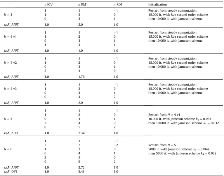
of the computations, several of them were chosen according to the spectral analysis of the time signal fromFig. 12. They range from three to six frequencies. The present implementation of the HB method in elsA imposes to set the same number of frequencies in each blade row. It would not be too difficult to overcome this constraint in order to reduce the number of frequencies in single frequency rows, such as the IGV and RD1 in the present case. This will be addressed in future versions of the software. The frequency combinations used are summarized inTable 3. This table shows the coefficients nk;ifrom Eq.(32)

chosen for each blade row. They are given by the immediately adjacent rows. For example, for N ¼ 4 v1, the frequency set is ½BPFRM1;2BPFRM1;3BPFRM1;4BPFRM1* in the IGV (i.e. j ¼ 1 in Eq.(32)) and in the RD1 (i.e. j ¼ 3) (which means that for these

rows the frequency content is mono-frequential) whereas, it is ½BPFIGV& BPFRD1;BPFIGV;BPFRD1;BPFIGVþ BPFRD1* in the RM1

(i.e. j ¼ 2 in Eq.(32)). It is clear that the different blade rows have different frequency sets. The upstream injection block and RD1 only solve for the BPF of the rotor and its harmonics, thus the classic Fourier analysis ensures that the best condi-tioning of the matrix A&1_{is given by evenly distributed time levels over the period T ¼ 1=BPF}

RM1. At this point, it should be

noted that 80 and 96 are multiples of 16 (i.e. blade number of RD1 minus blade number of IGV). Thus all the frequency com-binations ofTable 3for the rotor are multiples of the base frequency BPFIGV& BPFRD1. However, contrary to what is required

by a mono-frequential method, not all the intermediate harmonics need to be taken into account. For example, in a six-frequency set, the highest frequency is 2BPFRD1 which is also 12 , BPFð IGV& BPFRD1Þ. To perform a mono-frequential

harmonic computation taking into account 2BPFRD1, one would thus need BPFIGV& BPFRD1 as the fundamental and the 11

following harmonics, which implies a computation with 25 time samples. Such an approach would be inefficient, as the intermediate harmonics are not relevant here (see Fig. 12). The present multi-frequential HB method allows to perform the computation only on a set of chosen frequencies.

Fig. 13. Distribution of the time levels in the rotor for four frequencies over the base frequency BPFIGV& BPFRD1.

(19)

For such frequency ratios, the APFT algorithm provides good enough condition numbers of the matrix A&1_{(as shown in}

Table 3) and the use of the OPT algorithm was not mandatory. As it would be too long and tedious to present the time levels distribution for all the frequency sets,Fig. 13focuses on the three sets of four frequencies. It allows to observe, for the same number of frequencies, the impact of the frequency set on the APFT algorithm. The first remark that can be drawn from Fig. 13is that the APFT algorithm is not always needed: for N ¼ 4 v1, the best time levels distribution for the rotor is given by a uniform sampling whereas the APFT algorithm gives a condition number of 2:16. However, the gain is significant for the two other configurations: with evenly-spaced time levels, the condition numbers of the matrix A are respectively of 6:74 , 1015 _{for N ¼ 4 v2 and 2:62 , 10}15 _{for N ¼ 4 v3, while with the time levels issued from the APFT algorithm they go}

down to 1.76 and 2.0, respectively.

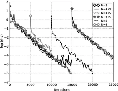
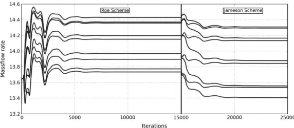
The convergence of the HB computations depends on the choice of the frequency set as shown inFig. 14, which depicts the convergence history at the peak-efficiency operating points. For all the computations, the residuals drop at least three orders of magnitude, which is considered to be enough to ensure convergence[45].Fig. 15plots the mass flow rate conver-gence for the first set of four frequencies. The instantaneous mass flow rates differ between the Roe and Jameson schemes. Grid convergence is actually not achieved for the Roe scheme but this not an issue as it is used only for initialization of the computation and the grid is fine enough for the target Jameson scheme. The latter is indeed considered as the reference scheme for the rest of the study since it is the scheme used for the DTS simulations.

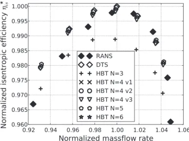
5.2.2.2. Time-averaged compressor performance. Figs. 16 and 17show the computed compressor map: the total pressure ratio

Pand the isentropic efficiency

g

isare plotted against the mass flow. They are non-dimensionalized by the values at the

max-imum-efficiency point. At blockage, the steady computations have a slightly higher mass flow rate and show a relative in-crease of the total pressure ratio by 1% near stall. Regardless of the number of frequencies, the overall agreement between the DTS and the HB technique for this variable is good. Indeed, the maximum relative difference is 0.4%. Up to the maximum

Fig. 15. Instantaneous mass flow rate history for HB N ¼ 4 v1.

(20)

isentropic efficiency, the steady curve matches well the one of the DTS, it then diverges to reach around 1% relative error near stall. The isentropic efficiency is more sensitive to the number of frequencies as there is a 1% difference for N ¼ 3, which re-duces below 0.1% for more frequencies. However, there are not many differences for more than four frequencies. Therefore, in term of global performance, the computations are converged with respect to the frequency content. Four frequencies are

Fig. 17. Non-dimensional isentropic efficiency mapg -is.

Fig. 18. Comparison of the entropy flow fields atg

(21)

consequently a minimum to compute correctly the aerodynamic performance. For clarity reasons and since the HB technique is an unsteady approach, the results from the mixing plane approach will not be plotted anymore.

5.2.2.3. Instantaneous results. Fig. 18shows the instantaneous entropy flow field for the maximum-efficiency operating point

g

-is¼ 1. For the HB computations, the computed passage is duplicated using phase-lag to check that the azimuthal phase-lag

boundary conditions ensure the continuity of the flow field between the original blade passage and the duplicated ones. All the wakes are correctly convected downstream and very few differences can be seen in the different flow fields. Some

Fig. 19. Rotor outlet: Azimuth-time map of the non-dimensional axial speed atg -is¼ 1.

(22)

numerical wiggles can be observed downstream the RM1/RD1 interface, but the higher the number of frequencies, the better the solution, as already shown by Sicot et al.[28].

5.2.2.4. Unsteady results. To analyze the prediction of unsteady row interactions within the rotor,Fig. 19shows the azimuthal evolution, in the relative frame, of the non-dimensional axial speed downstream of the rotor, as a function of time, for the DTS, HB N ¼ 3, HB N ¼ 4 v1 and HB N ¼ 6 computations. In this diagram, the horizontal bands of low axial speed correspond to the wakes of the rotor itself, which remains steady in the relative rotating frame. The IGV wakes, cropped by the rotor and convected within the passage can also be observed as ‘‘oblique strips’’ of low velocity. ComparingFig. 19(a) and (b) clearly shows that only three frequencies are not sufficient to reproduce correctly the time and space evolutions of the wakes. The

Fig. 21. Rotor outlet: Non-dimensionalqtime signal comparison between DTS and HB at mid pitch.

(23)

four-frequency set (Fig. 19(c)) gets the rotor and IGV wakes clearly visible, but a bit more twisted than in the reference solu-tion. The minimum value is also under-predicted by 3.6%. The six-frequency solution (Fig. 19(d)) has the same features as the four-frequency one, except that the IGV wake is slightly better predicted and the minimum is now correct.

To facilitate comparisons between the different HB frequency sets and the DTS, the azimuthal evolution of the non-dimensional fluid density

q

along a line of constant radius is plotted inFig. 20for t ¼ 0. This amounts to extracting a vertical line at t ¼ 0 inFig. 19, but this time density was chosen as it is a conservative variable and it is more subject to variations

Fig. 23. Comparison of both algorithms for N ¼ 6 HB computations at the rotor outlet.

Table 4

Frequency combination coefficients to compute only harmonics of the fundamental blade-passing frequencies.

nIGV nRM1 nRD1 Initialization

1 1 0 Restart from steady computation

N ¼ 4 v4 0 2 1 15,000 it. in Roe second order scheme

2 3 0 then 10,000 it. in Jameson scheme

0 4 2

jðAÞ APFT 1.0 2.73 1.0

1 1 0

0 2 1 Restart from N ¼ 4 v4

2 3 0 5000 it. in Jameson scheme k4¼ 0:064

N ¼ 6 v2 0 4 2 then 5000 it. in Jameson scheme k4¼ 0:032

3 5 0

0 6 3

jðAÞ APFT 1.0 4.03 1.0

(24)

than the others. For the sake of clarity, the results for the second four-frequency (N ¼ 4 v2) and five-frequency sets are not shown here. The results for three frequencies oscillate around the values of the DTS. Underlying the comments made on the convergence history, the two sets of four frequencies give quite different azimuthal results. Both results for four frequencies

Fig. 25. Distribution of the time levels over the period of the RD1.

Fig. 26. Non-dimensional total pressure ratio mapP-_.

Fig. 27. Non-dimensional isentropic efficiency mapg -is.

(25)

follow the variations of the DTS. The results for the first set of four frequencies are quite fair. Given the quality of the results given by HB N ¼ 4 v1, it is surprising that HB N ¼ 6 v1 does not perform better since its frequency content is merely an enrichment of HB N ¼ 4 v2.

To further analyze unsteady interactions within the rotor, a probe was positioned downstream of the rotor in the middle of the passage. The unsteady density signal is plotted inFig. 21. For four frequencies, the variations of non-dimensional

q

in time are almost the same and are matching the evolution of the DTS. To have an accurate approximation of the flow field, four frequencies seems to be the minimum required.

The unsteady pressure coefficient Cpat mid-span of the rotor blade is now studied, and the contribution of the upstream

and downstream rows are isolated.Fig. 22(a) depicts the mean value on the rotor blade along the normalized curvilinear coordinates for DTS, HB N ¼ 3, HB N ¼ 4 v1 and HB N ¼ 6, whereas (b) and (c) plot the amplitude evolution for, respectively,

Fig. 28. Comparison of the entropy flow field atg

-is¼ 1:0 and t ¼ 0.

Fig. 29. Comparison of the azimuthal evolution of non-dimensionalqatg -is¼ 1.

(26)

Fig. 30. Comparison of the temporal evolution of non-dimensionalqatg -is¼ 1.

Fig. 31. Azimuth-time map of the axial speed atg -is¼ 1.

(27)

the upstream and the downstream blade passing frequency. The leading edge corresponds to s ¼ 0 or s ¼ 1, whereas the trailing edge is located at s ¼ 0:5. Between 0.0 and 0.5 is the suction side and between 0.5 and 1 is the pressure side. As shown inFig. 22(a), three frequencies are enough to capture the mean Cpvalue around the blade. All four-frequency sets

and the six-frequency set fit perfectly the DTS amplitudes for the passing frequency of the IGV blades, except for a wiggle at the end of the suction side. Concerning the amplitudes of the passing frequency of RD1, HB N ¼ 4 v1 and HB N ¼ 6 cor-rectly predict the suction side and HB N ¼ 4 v3 under-predicts the maximum of the amplitude. All frequency sets have trou-ble predicting the amplitude right after the trailing edge at the pressure side. Surprisingly, it is HB N ¼ 4 v3 that is the best match, whereas one would have rather expected HB N ¼ 6 to be so.

5.2.2.5. Comparison of the algorithms. Table 3shows that the condition number

j

ðAÞ for six frequencies with the APFT algo-rithm is the highest amongst the chosen frequency combinations. The OPT algoalgo-rithm allows to reduce

j

ðAÞ in the rotor from 2.72 to 2.43.Fig. 23plots the azimuthal evolution of the density for the different algorithms and for six frequencies, along with the evolution of the DTS. The discrepancies are small and are mainly located around 58.6". Given the closeness of the two harmonic solutions, the APFT algorithm gives, in this case, good enough condition numbers to perform HB computations. 5.2.3. A priori computations: HB computations with only the BPFs of the adjacent rows

The previous computations were made in the ideal case in which the flow spectrum is known a posteriori. This allows to choose the frequencies that are the most likely to give the best results. From this standpoint, HB N ¼ 4 v1 is an especially good example. However, in practice, one does not have such an information. One solution would be to consider a significant number of harmonics of all rows BPF and their combinations. However the curse of dimension prevents of doing so as the total number of frequencies would quickly be too high. The usual first guess consists in using only the blade passing frequencies of the adjacent rows. This may appear as a great simplication but one has to keep in mind that HB methods are reduced-order models and provide much more information than steady computations, but not necessarily as much as

(28)

a classical time-accurate computation. This leads to two new sets of frequencies (one of four and one of six frequencies), which are summarized inTable 4.

Figs. 24 and 25 show the associated time distributions found thanks to the APFT algorithm on both base frequencies (BPFIGVand BPFRD1) with the associated condition numbers.

As done previously, the first step consists in checking the aerodynamic values.Figs. 26 and 27plot respectively the total pressure ratio and the isentropic efficiency for the new frequencies. Regarding both values, the relative error margins are almost the same as in the previous HB computations.

The resulting entropy flow fields for these new frequency sets are shown inFig. 28. The reference DTS field is also plotted as a reminder in28(a). They do not show any significant discrepancy with the previous figures. In compliance with the com-ments made onFig. 18, some wiggles manifest at the interface RM1/RD1 with HB N ¼ 4 v4, but disappear as the number of frequencies is increased.Figs. 29 and 30compare respectively the azimuthal and temporal evolution of the new frequency sets with the old ones of corresponding number of frequencies. It comes out fromFig. 29that, in this case, the importance of the blade passing frequencies cannot be denied, since with enough harmonics of the passing frequencies (top) the DTS curve is very well-matched by HB N ¼ 6 v2. With fewer harmonics (bottom), HB N ¼ 4 v4 behaves like HB N ¼ 4 v2.

Fig. 30shows no noticeable improvement (nor deterioration) of the local time evolution with the change of frequencies. The time-azimuth maps are given inFig. 31. The main difference lies the shape of the bubble in the wake of the rotor, which is better captured by the six-frequency set.

The previous figures point that the performances of HB N ¼ 6 are not as good as HB N ¼ 6 v2.Fig. 32shows the Cpfor both

six-frequency sets. The mean value evolution in32(a) exhibits no difference between the two frequency sets. The same re-mark can be made for the IGV BPF in32(b) except for a minor difference at 80% of the suction side. Concerning RD1’s BPF in 32(c), HB N ¼ 6 v2 gives a better overall match with the DTS than HB N ¼ 6 v1 and especially in the last third of the pressure side.

5.2.4. Computational gain

Fig. 33shows that the HB computations allow a reduction of the CPU cost by a factor 4.5 for four frequencies, the gain being higher with fewer harmonics. However, it should be kept in mind that the reference DTS simulations are done on a 2

p

=16 periodic sector, whereas practical turbomachinery configurations usually do not have such periodicity, thus requiring simulations on the whole 360" machine. In this case, an additional factor 16 in gain can thus be estimated, suggesting a gain of almost two orders of magnitude. Since the present mesh does not allow multigrid computation, it is also possible to expect a gain even higher as multigrid is a very efficient convergence-acceleration technique for steady computations. This leaves room for further improvements in CPU time reduction.

6. Conclusion

Classical time integration schemes for the Navier–Stokes equations are based on the hyperbolic nature of the problem: the state at a given time step is deduced from the previous one. For periodic flows, this approach is not well suited, as past and future do not have the same meaning. The harmonic balance approach relies on direct and inverse Fourier transforms to turn the time-marching problem into the coupled resolution of several mathematically steady problems representing snap-shots of the unsteady solution. When unsteadiness is related to a single (main) frequency and its harmonics, Fourier analysis leads to a natural choice for time instants: they are evenly spaced over the period. In this case, the mathematical problem is numerically well-posed, which means that the conditioning of the operators ensures that the technique converges.

When several arbitrary frequencies are considered, as in multi-stage turbomachines, the HB approach can be theoretically extended, if (and only if) time instants are chosen such that the transformation matrix remains invertible. In the available literature, two approaches based on evenly spaced instants over the shortest period of interest are used: either 2N þ 1 or

(29)

3N þ 1 time samples are considered for N frequencies. Oversampling is left away for its higher computational cost and uni-form sampling can lead to stability issues. As a consequence, the choice of the time sampling remains a key point.

In this paper, a non-uniform time-sampling approach has been proposed for the time-domain multiple-frequency har-monic balance method. Such an approach is particularly efficient for multiple-harhar-monics problems where the frequencies are widely separated, thus extending the application range of the method.

It is first demonstrated that the time sampling has a major effect on the stability of the method, due to the condition num-ber of the Fourier transform matrix. To tackle this issue, two algorithms have been derived to find appropriate non-uniform sampling: the APFT algorithm improves the Fourier matrix orthogonality in order to reduce its condition number, while the OPT algorithm directly minimizes the condition number thanks to a gradient-based optimization method.

A channel flow test case with oscillating outlet pressure is then used to demonstrate the ability of the proposed algo-rithms to accurately capture a flow driven by two coprime frequencies, thus alleviating the stability issues that can arise even for such a simple problem.

Finally, the flow in a multi-stage axial compressor is computed to prove the maturity of the method. It is shown that non-linear flows can be modeled to engineering accuracy with only four frequencies. This conclusion holds for subsonic flows: when shocks are present, previous studies with the proposed approach have shown that accurate and cost-effective solu-tions can still be obtained, but at the expense of an increased number of harmonic[4]. In the present case, the HB method is about 70 times faster than a classical time-marching computation over the whole annulus, thanks to the efficient spectral-integration scheme and to the generalized phase-lag boundary conditions. The conclusions obtained for the present quasi-2D case have been extended to 3D geometries without any new assumption[40].

It should be emphasized that the method is still a reduced-order model, as only selected frequencies are computed. In this respect, a priori computations using only adjacent rows BPFs are presented, showing good agreement with the reference time-marching solution, which suggests that the HB method can be used in an industrial context. However, full confidence in the HB solution can only be established by comparison with computations using more frequencies, quite similarly to grid independence demonstration.

Another point of interest is the shape optimization of industrial turbomachinery to improve their efficiency. Among other optimization approaches, gradient based optimization techniques using adjoint calculations have become popular for the de-sign of complex systems parameterized by a large number of dede-sign variables since the pioneering work of Jameson[46]. However, both computational cost and technical difficulties can be prohibitive for unsteady flows: the adjoint system has to be solved in a reverse way and Navier–Stokes solutions have to be stored during the iterative process. These problems remain for periodic flows with classical time marching integration schemes. With the considered harmonic methods, com-puting sensitivities is much simpler since the residuals to be derived with respect to the state variables and the mesh nodes coordinates are similar to RANS equations of which adjoint state is classically computed. As a consequence, the computa-tional cost for adjoint sensitivities of such flows is affordable and the overall complexity is finally moderate. Duta et al. [47]have used this technique in the context of aeroelastic turbomachinery design and a wide range of potential applications for the HB method is now opened.

Acknowledgments

The present harmonic balance formulation was developed thanks to the support of the Direction des Programmes Aéronau-tiques Civils(French Civil Aviation Agency) and of the Aerospace Valley (Midi-Pyrénées and Aquitaine world competitiveness cluster). The authors would also like to thank SNECMAfrom the SAFRAN GROUPfor their kind permission to publish this study.

References

[1] K. Hall, W.S. Clark, C.B. Lorence, A linearized Euler analysis of unsteady flows in turbomachinery, Journal of Turbomachinery 116 (1994) 477–488. [2] W.S. Clark, K.C. Hall, A time-linearized Navier–Stokes analysis of stall flutter, Journal of Turbomachinery 122 (2000) 467–476.

[3] L. He, Harmonic solution of unsteady flow around blades with separation, AIAA Journal 46 (2008) 1299–1307.

[4] G. Dufour, F. Sicot, G. Puigt, C. Liauzun, A. Dugeai, Contrasting the harmonic balance and linearized methods for oscillating-flap simulations, AIAA Journal 48 (2010) 788–797.

[5] N. Gourdain, L. Gicquel, R. Fransen, E. Collado, T. Arts, Application of RANS and LES to the prediction of flows in high pressure turbine components, in: ASME Turbo Expo, GT2011-46518, Vancouver, Canada, 2011, pp. 1773–1785.

[6] P. Sagaut, S. Deck, Large-Eddy simulation for aerodynamics: status and perspectives, Philosophical Transactions of the Royal Society A 367 (2009) 2849–2860.

[7] L. He, Fourier methods for turbomachinery applications, Progress in Aerospace Sciences 46 (2010) 329–341.

[8] L. He (Ed.), Special Issue: Fourier-based method development and application, International Journal of Computational Fluid Dynamics, in press. [9] L. He, W. Ning, Efficient approach for analysis of unsteady viscous flows in turbomachines, AIAA Journal 36 (1998) 2005–2012.

[10] W. Ning, L. He, Computation of unsteady flows around oscillating blades using linear and nonlinear harmonic Euler methods, Journal of Turbomachinery 120 (1998) 508–514.

[11] K.C. Hall, J.P. Thomas, W.S. Clark, Computation of unsteady nonlinear flows in cascades using a harmonic balance technique, AIAA Journal 40 (2002) 879–886.

[12] A. Gopinath, A. Jameson, Time spectral method for periodic unsteady computations over two- and three-dimensional bodies, in: 43rd Aerospace Sciences Meeting and Exhibit, AIAA Paper 2005-1220, Reno, USA, 2005.

[13] J. Tyler, T. Sofrin, Axial flow compressor noise studies, Society of Automotive Engineers Transactions 70 (1962) 309–332.

[14] A. Gopinath, E. Van Der Weide, J. Alonso, A. Jameson, K. Ekici, K. Hall, Three-dimensional unsteady multi-stage turbomachinery simulations using the harmonic balance technique, in: 45th AIAA Fluid Dynamics Conference and Exhibit, AIAA Paper 2007-0892, Reno, USA, 2007.