Science Arts & Métiers (SAM)
is an open access repository that collects the work of Arts et Métiers Institute of
Technology researchers and makes it freely available over the web where possible.
This is an author-deposited version published in: https://sam.ensam.eu Handle ID: .http://hdl.handle.net/10985/7219
To cite this version :
Anna DUPLEIX, Andrzej KUSIAK, Mark HUGHES, Frédéric ROSSI - Measuring the thermal properties of green wood by the transient plane source (TPS) technique - Holzforschung - Vol. 67, n°4, p.Pages 437–445 - 2013
Any correspondence concerning this service should be sent to the repository Administrator : [email protected]
Measuring the thermal properties of green wood
by the transient plane source (TPS) technique
Abstract: The thermal properties of wood in the green state have been determined by the transient plane source (TPS)
technique. Data are presented on thermal conductivity ( λ ),
heat capacity ( C ), and thermal diffusivity ( κ ) at moisture
contents (MCs) above the fiber saturation point, which are
based on measurements using the HotDisk ® apparatus.
Four wood species (Douglas fir, beech, birch, and spruce) were tested, and the results are compared with literature data and those obtained by the flash method. A linear
relationship was found between the thermal properties λ ,
C , and κ on the one hand and MC on the other. Equations
predicting the thermal values as a function of MC and
wood anisotropy are presented. Wood C and λ increase
with MC, but wet wood diffuses heat more rapidly than dry wood.
Keywords: green wood, heat capacity, HotDisk ® , thermal
conductivity, thermal diffusivity, transient plane source (TPS)
*Corresponding author: Anna Dupleix, Arts et Metiers ParisTech
LaBoMaP, Rue Porte de Paris, F-71250 Cluny, France, Phone: + 33 3 85 59 53 27, Fax: + 33 3 85 59 53 85, e-mail: [email protected]
Anna Dupleix and Mark Hughes: Department of Forest Products Technology , School of Chemical Technology, Aalto University, FI-00076 Aalto , Finland
Andrzej Kusiak: Universit é Bordeaux 1 , I2M, Esplanade des Arts et M é tiers, F-33405 Talence Cedex , France
Fr é deric Rossi: Arts et Metiers ParisTech LaBoMaP , Rue Porte de Paris, F-71250 Cluny , France
Introduction
Thermal conductivity ( λ ), heat capacity ( C ), and thermal
diffusivity ( κ ) are the most important properties that
char-acterize the thermal behavior of a material and also that of wood (Suleiman et al. 1999 ; Olek et al. 2003 ; Sonderegger et al. 2011 ). At moisture contents (MCs) between 0 % and fiber saturation point (FSP), wood is considered to be a
good insulating material with low λ , moderate C , and
con-sequently low κ . The porosity of wood has a low λ because
the λ of air filling the void spaces is lower ( λ air = 0.0261
W m -1 K -1 at 300 K) than that of the cell wall (Rohsenow
et al. 1973 ). Heat flows preferentially through the wood cell walls, which act like heat bridges, whereas the air present in the lumens below the FSP forms a barrier to heat flow (Kollmann and C ô t é 1968 ).
The thermal properties of wood are affected by a range of factors including the extractive content, grain direction, knots, checks, microfibril angle, growth rings, ray cells, anisotropy, wood species, and porosity. The MC and tem-perature are also influential with this regard (Suleiman
et al. 1999 ). Both λ and C increase linearly with
tempera-ture, but the λ increment is smaller than that of C (Harada
et al. 1998 ; Simpson and TenWolde 1999 ). The present study is focused on the effect of anatomical orientation (radial or tangential) and MC on wood ’ s thermal properties.
Influence of anisotropy
The influence of wood anisotropy on transverse conduc-tivity is controversial. Some authors (Siau 1971 ; Simpson and TenWolde 1999 ; Suleiman et al. 1999 ) report the same
λ values in the radial ( λ R ) and tangential ( λ T ) directions, whereas other authors claim that transverse conductivity is higher in the R than in the T direction (see Table 1 ). The
ratio of λ R and λ T is thought to be governed by the volume
of ray cells in hardwoods and the volume of latewood in
softwoods (Steinhagen 1977 ). Similar λ R and λ T data were
obtained for hardwood species with a rather uniform wood structure or a low amount of latewood, such as in young softwoods (Suleiman et al. 1999 ). However, studies
on beech and spruce support the concept that λ R
pre-dominates (Sonderegger et al. 2011 ). Logically, there is no influence of orientation on specific heat, as this property is mainly dependent upon the cell wall material itself. Consequently, there is hardly any influence of density on c (Sonderegger et al. 2011 ); neither is there much
varia-tion from one species to another (Jia et al. 2010 ). As κ is
proportional to λ , it is logical that diffusivity is also
aniso-tropic because ρ and c are both isotropic properties
(Stein-hagen 1977 ). Therefore, the κ R should be higher than κ T
because of the lower tangential λ T (Kollmann and C ô t é
1968 ). However, as with λ , some findings do not
2 A. Dupleix et al.: Measuring thermal properties by TPS
Influence of MC
The conductivity of water ( λ water = 0.613 W m -1 K -1 at 300 K
(Rohsenow et al. 1973 ) is higher than that of air. Accord-ingly, wood conductivity increases with higher MC, as there is a linear relationship between these parameters
(Table 1). For beech and spruce, the R 2 of this relationship
is ~ 0.95 – 0.99 (Sonderegger et al. 2011 ). Free water
con-ducts more heat than bound water; thus, the λ increment
is steeper above FSP (Siau 1971 ). The presence of water strongly affects the heat capacity of wood because of the high of water c water = 4.18 kJ kg -1 K -1 at 300 K (Rohsenow et al.
1973 ). As a first approximation, the specific heat c of wet wood can be calculated using a simple rule of mixtures by adding the specific heat c water and c 0 (for oven-dried wood)
in their relative proportions:
c = wc water + (1- w ) c 0 (1)
where w is the weight fraction of water in wood based on the mass of wet wood. Expressing w as a function of m (MC in % /100) gives rise to Eq. (2), and substituting w in Eq. (1) gives rise to Eq. (3) (Kollmann and C ô t é 1968 ).
w = m /(1 + m ) (2)
c = ( c water m + c 0 )/(1 + m ) (3) Eqs. (1) and (3) consider wet wood to be a mixture of two independent materials; however, this may be an oversimplification, and some authors have suggested that this relationship only holds true when the MC is > 5 % (Jia et al. 2010 ; Sonderegger et al. 2011 ). Table 1 summarizes the different relations between c and MC. As indicated,
some authors propose an additional coefficient ( A c ) to
take into account the energy lost during the wetting of the cell wall due to the creation of H bonds between cellulose and water (Simpson and TenWolde 1999 ; Sonderegger
et al. 2011 ). However, A c values vary among authors and
are only valid below FSP. Other authors modify the coef-ficients in the rule of mixtures as a function of MC (Siau 1995 ; Koumoutsakos et al. 2001 ). However, the correlation
between specific heat c and w /(1 + w ) was linear in case of
beech and spruce (Sonderegger et al. 2011 ). Studies
focus-ing on heat diffusion κ of wet and dry wood are scarce.
According to Kollmann and C ô t é (1968) , κ decreases
slightly with MC, with a very low inclination (-0.01) (see Table 1).
Measurement methods of thermal properties
The guarded hot plate method has proven to be the most accurate procedure for measuring unidirectional thermal
conductivity in all kind of materials under conditions of
steady-state heat conduction (Speyer 1994 ; Bu č ar and
Stra ž e 2008 ). Establishing a steady-state heat flow, when a stable temperature gradient is developed (ISO 8302 ), takes ~ 10 min in the case of a 200-mm-thick wood sample. This condition can be achieved by maintaining MC values below the FSP (up to 20 % MC) by controlling the relative humidity (Sonderegger et al. 2011 ). However, testing green wood under such conditions is impossible without risking the formation of a perturbing moisture gradient within the sample.
Meanwhile, the thermal properties of green wood can be measured using transient methods within a couple of
Predicting equations for the thermal properties indicated
Required conditions (literature a )
λ (W m -1 K -1 ) λ = G (0.2 + 0.4 m ) + 0.02 5 % < MC < 35 % (1); MC < 25 % (2); MC < 40 % (3, 4) λ = G (0.2 + 0.5 m ) + 0.02 MC > 40 % (3, 4) λ R = 0.086 + 0.108 m MC < 20 % , spruce (1) λ T = 0.092 + 0.235 m λ R = 0.120 + 0.193 m MC < 20 % , beech (1) λ T = 0.071 + 0.128 m λ R / λ T 13 % fir (5) 11 % oak (5) 3 % – 20 % (1) 5 % – 10 % (3) c (kJ kg -1 K -1 ) c = (( c water m + c 0 )/(1 + m )) + A c MC < 5 % , A c = 0 (1, 6); 5 % < MC < FSP, A c < 0 (1); MC < FSP, A c = m (-6.191 + 2.36 × 10 -2 T -1.33 m ) (2) c = (4.15 m + 1.260)/(1 + m ) MC < 5 % (7, 8) c = (5.859 m + 1.176)/(1 + m ) 5 % < MC < 30 % (7, 8) c = (4.185 m + 1.678)/(1 + m ) MC > 30 % (7, 8) c = (0.0364 m )/(1 + m ) + 1.245 MC < 17 % , spruce (1) c = (0.0337 m )/(1 + m ) + 1.134 MC < 17 % , beech (1) c 0 = 1350 20 ° C (4) c 0 = 1590 20 ° C (9) c 0 = 1250 20 ° C (10) c 0 = 1176 20 ° C (6) κ (m 2 s -1 ) κ = (- m + 0.199)10 -6 ρ = 200 kg/m 3 (3) κ = (- m + 0.167)10 -6 ρ = 400 kg/m 3 (3) κ = (-0.9 m + 0.153)10 -6 ρ = 600 kg/m 3 (3) κ = (-0.6 m + 0.143)10 -6 ρ = 800 kg/m 3 (3)
Table 1 Literature equations predicting the influence of MC, density, and transversal directions on λ , C , and κ .
a Literature: (1) Sonderegger et al. (2011), (2) Simpson and TenWolde (1999), (3) Kollmann and C ô t é (1968), (4) Siau (1971), (5) Incropera et al. (2011), (6) Jia et al. (2010) , (7) Siau (1995) , (8) Koumoutsakos et al. (2001) , (9) Steinhagen (1977) , (10) Harada et al. (1998) ; G = ( m 0 / V μ )/ ρ water = specific gravity based on the weight of the oven-dried wood, m 0 , and volume at MC, V μ (no dimension).
seconds. The transient hot wire (THW) and transient hot
strip (THS) techniques can provide values for λ and κ from
the temperature measured locally by a thermocouple sandwiched between two specimens and located next to the electrified wire or strip that dissipates heat to the sur-rounding material. The flash method is another transient
technique that can provide κ values from the temperature
change on the rear face of a sample exposed to a laser or a lamp that supplies heat through the front face. The tem-perature change can be measured locally by a thermocou-ple or an infrared camera to obtain the whole temperature field on the rear face of the sample.
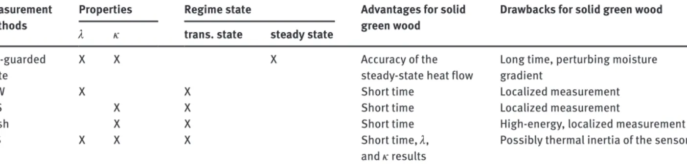
The advantage of the TPS technique over the other transient methods cited above is that it is based on the measurement of the average temperature of the heated surface of the sample. It is particularly important in the case of anisotropic materials such as wood. Moreover, it permits the simultaneous characterization of κ , λ , and C . Table 2 compares the advantages and disadvantages of each method in measuring the thermal properties of green wood.
The general theory of TPS has been comprehen-sively described by Gustafsson (1991) . The TPS tech-nique entails recording the resistance change as a function of time of the heat source, in form of a disk, which serves as the measuring sensor. The TPS element is sandwiched between two specimens while an electri-cal current is passed through it with sufficient power to slightly increase its temperature (between 1 and 2 K). The temperature coefficient of the resistivity (TCR) of the sensor is known; thus, its resistance change gives information on its temperature variation. As with the THS and THW techniques, the solution of the equations involved in the TPS method relies on the assumption that the sensor is placed in an infinite medium. This assumption implies that the time of transient record-ing ends before heat reaches the outer boundaries of the sample to avoid edge effects and that the sample
size, which can be arbitrary, ensures that the distance from the sensor edges to the nearest sample boundary
exceeds the probing depth Δ p [Figure 1 , Eq. (6)]
(Gustavs-son et al. 2000 ):
Δ p = 2( κ t max )
1/2 (6)
where t max is the total time of experiment. The benefit of
the TPS technique lies in its ability to combine both heat source and temperature sensor in the same TPS element, thereby ensuring a better accuracy of the thermal trans-port measurement compared with the THS or THW
methods. The TPS technique consists of measuring λ and
κ , whereas C is calculated from the relationship κ = λ / C . Fitting the TPS experimental results with the analytical
models presented by Gustafsson (1991) leads to λ and κ
values.
Specific objectives of the study
The aim of the work reported herein was to investigate the transverse (radial and tangential) thermal conduc-tivity ( λ ), heat capacity ( C ), and thermal diffusivity ( κ ) of the green wood of the species beech, birch, Douglas fir, and spruce at MC above FSP. The TPS technique was in focus. The literature data with TPS are limited to dry wood (Suleiman et al. 1999 ); thus, the present article intends to deliver data above FSP. Empirical equations
for predicting the relationship between λ , C , and κ and
MC above the FSP should be calculated. The rationale for conducting this study was to render possible numerical models that simulate the transverse IR heating of green wood based on accurate thermal property data (Dupleix et al. 2012 ). For this reason, only the transverse tions will be tested because they are the main direc-tions of heat flow. The lack of data in the literature on the thermal properties of green wood provided the main impetus for this study.
Measurement methods
Properties Regime state Advantages for solid green wood
Drawbacks for solid green wood λ κ trans. state steady state
Hot-guarded plate
X X X Accuracy of the
steady-state heat flow
Long time, perturbing moisture gradient
THW X X Short time Localized measurement
THS X X Short time Localized measurement
Flash X X Short time High-energy, localized measurement
TPS X X X Short time, λ ,
and κ results
Possibly thermal inertia of the sensor
4 A. Dupleix et al.: Measuring thermal properties by TPS
Materials and methods
List of symbols
c Specific heat (kJ kg-1 K-1)
c0 Specific heat of oven-dried wood (kJ kg
-1 K-1)
C = ρc Heat capacity (J m-3 K-1)
CR Radial heat capacity (J m-3 K-1)
CT Tangential heat capacity (J m-3 K-1)
G Specific gravity (no dimension)
κ = λ/C Diffusivity (m2 s-1) κR Radial diffusivity (m2 s-1) κT Tangential diffusivity (m2 s-1) λ Transverse conductivity (W m-1 K-1) λR Radial conductivity (W m-1 K-1) λT Tangential conductivity (W m-1 K-1)
m MC in%/100 (no dimension)
r Probe radius (mm)
ρ Density (kg m-3)
tmax Total time of experiment (s)
τ Characteristic time (s)
w Fraction of water in wet wood (no dimension)
Samples
Knot-free samples of beech [ Fagus sylvatica (L)], birch [ Betula
pen-dula (Roth)], heartwood of Douglas fi r [ Pseudotsuga menziesii (Mull)
Franco], and spruce [ Picea albies (L.) Karst] were studied. The sam-ples were split from the same freshly cut tree in the tangential ( T )
and radial ( R ) directions with respect to grain orientation and were sawn to the initial shape of a block with dimensions of 44 × 44 × 30 mm 3 . Each sample was then cut in two parts, giving rise to identical samples of 44 × 44 × 15 mm 3 (Figure 1). Both top and bottom samples will have the same thermal transport behaviors because of their sym-metrical growth ring geometry.
Method
The pretesting of each sample was performed to carefully adjust the parameters cited in Table 3 as a function of the chosen probe. This time-consuming process of adjusting the settings was, however, essential for the TPS measurement method because of its numer-ous parameters, which would distort the results, if inappropriately selected (Olek et al. 2003 ). Once values obtained are ensured to be representative of wood thermal properties, repetitions of the test were performed until hardly any change in the standard deviation (SD) was observable. Hence, each point plotted in the graphs in the Results and Discussion section represents the average of 30 indi-vidual measurements taken at fi ve diff erent locations of the sample. The TPS element sandwiched between two samples delivers a heat fl ow mainly radially for the sample cut in the T direction and vice versa.
Moisture content
The samples were maintained in the green state by vacuum packing until testing. Samples were subsequently placed in a hot and wet air fl ow for diff erent durations to obtain a wide range of MCs above the Figure 1 Sampling identical samples and TPS measurement configuration showing probing depth Δ p .
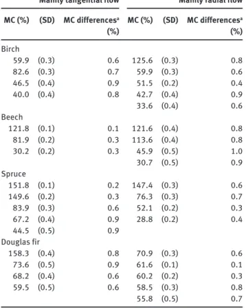
FSP. The slow drying procedure should have ensured that the MC is homogeneous throughout the sample, thus minimizing any possible side-eff ects caused by moisture gradient. MC was measured with the double weighing method, where the initial weight was the weight at the time of the experiments. This limited the time of the measure-ments to a couple of seconds, and placing the sample underneath the cover of the TPS device ensured that heat transfer by convection was avoided, resulting in the drying of the samples during the experiment. This assumption was confi rmed by measuring the MC at the start and at the end of the experiment. The MC diff erence never exceeded 1 % , thus the eff ect of drying during the experiments is negligible. The MC values are the means of fi ve determinations aft er the TPS measure-ment on each of the fi ve locations tested for a sample (Table 4 ).
TPS parameters Values and units
TCR 0.005 K -1
Temperature increase 1 – 2 K
Measurement time τ 80 – 320 s
Probing depth Δ p ~ 10 mm
Probe radius r 6.4 mm (model 5501)
Input power 0.01 – 0.05 W
External temperature 22 ° C
Table 3 Summary of the parameters used during the experiments with TPS.
Mainly tangential flow Mainly radial flow MC ( % ) (SD) MC differences a ( % ) MC ( % ) (SD) MC differences a ( % ) Birch 59.9 (0.3) 0.6 125.6 (0.3) 0.8 82.6 (0.3) 0.7 59.9 (0.3) 0.6 46.5 (0.4) 0.9 51.5 (0.2) 0.4 40.0 (0.4) 0.8 42.7 (0.4) 0.9 33.6 (0.4) 0.6 Beech 121.8 (0.1) 0.1 121.6 (0.4) 0.8 81.9 (0.2) 0.3 113.6 (0.4) 0.8 30.2 (0.2) 0.3 45.9 (0.5) 1.0 30.7 (0.5) 0.9 Spruce 151.8 (0.1) 0.2 147.4 (0.3) 0.6 149.6 (0.2) 0.3 76.3 (0.3) 0.7 83.9 (0.3) 0.6 52.1 (0.2) 0.3 67.2 (0.4) 0.9 28.8 (0.2) 0. 4 44.5 (0.5) 0.9 Douglas fir 158.3 (0.4) 0.8 70.9 (0.3) 0 .6 73.6 (0.5) 0.9 61.6 (0.1) 0.1 68.2 (0.4) 0.6 60.2 (0.2) 0.3 59.5 (0.5) 0.6 58.5 (0.3) 0.8 55.8 (0.5) 0.7
Table 4 Mean MC, SD, and difference of MC between the start and the end of experiment calculated on five tested locations for the wood samples indicated.
a Between start and end of experiments.
TPS device
The HotDisk ® Thermal Constants Analyser ® was from I2M (Bordeaux, France). The 13- μ m-thick, 6.403-mm-radius, spiral-shaped TPS element of known TCR was of nickel foil covered by a polymer Kap-ton, which is highly temperature-resistant and electrically insulat-ing (Figure 1). Clamps were used to ensure good and reproducible thermal contact. Before the experiments, a Wheatstone bridge com-posed of the TPS element as one resistor was balanced to reset the TPS element resistance to 0. To enable the wood samples to recover isothermal conditions between measurements, a relaxation time was set on 36 times the duration of the transient recording, as rec-ommended in the HotDisk ® user ’ s manual. The experiments were performed at constant room temperature. The parameters are listed in Table 3.
The probe size was chosen to be as large as possible to widen the probed area and obtain average values representative of the thermal properties with minimum disturbance induced by structural hetero-geneities (e.g., annual growth rings, diff erences of densities between earlywood and latewood). However, the larger probe size, the longer characteristic time τ [Eq. (7), where r is the probe radius] and there-fore the longer the measurement time. Thus, a compromise had to be made between the largest possible probe size and the limited meas-urement time to avoid any edge eff ects and prevent the drying of the sample.
τ = r 2 / κ (7)
Results
Transverse conductivity ( λ ), heat capacity ( C ), and thermal
diffusivity ( κ ) are presented in Figures 2 – 4 , respectively, as calculated by the equations in Table 5 . The repeatabil-ity of the experiments is demonstrated by moderate SDs (error bars). The predictive equations for λ , C , and κ are
presented in Table 5 as obtained by the HotDisk ® method
in the present article and by the flash method according to Beluche (2011) . As clearly visible, the relationships with MC above the FSP are good, as expressed by the high
coef-ficients of determination ( R 2 ). The equations are
particu-larly useful for understanding heat transfer in wood in the green state (Table 5).
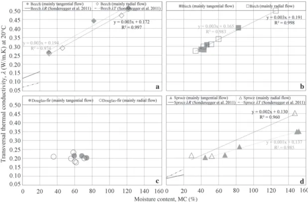
Figure 2 compares the λ values obtained in this work
with those obtained by the steady-state guarded hot plate method (Sonderegger et al. 2011 ). Apart from spruce, the
λ experimental values continuously match results from the literature (Sonderegger et al. 2011 ), but the values are slightly higher for all other species. There is no significant
difference in λ between the radial and the tangential
direc-tions for wood in the green state – apart from spruce. It seems that the presence of free water in the cell overrides any effects arising from the anisotropy of the wood. The exception in the case of spruce might be explained by
6 A. Dupleix et al.: Measuring thermal properties by TPS
the presence of ray cells that promote heat transfer in the radial direction ( λ R > λ T ).
Figure 3 compares the C values obtained with the results of Sonderegger et al. (2011) and oven-dried values
at 20 ° C referred to in the literature (Kollmann and C ô t é
1968 ; Steinhagen 1977 ; Jia et al. 2010 ). The gradients of the linear relationships between C and MC above FSP are steeper than below the FSP (results from literature),
most probably arising from the dominating effect of the free water. The scattered results for Douglas fir and spruce can be interpreted to mean that C in the green state is not unique for all wood species. There are probably two dif-ferent ranges of C values for hardwoods and softwoods: the former in the green state would need more energy for heating than softwoods. This behavior is different from that described in the literature below the FSP.
Figure 2 Thermal conductivity ( λ , in W m -1 K -1 ) at green state with HotDisk ® of (a) beech, (b) birch, (c) Douglas fir, and (d) spruce.
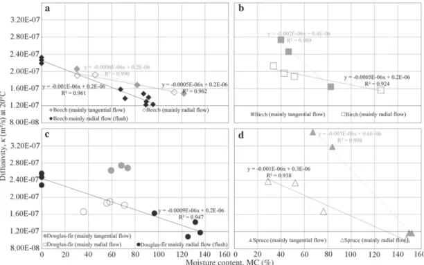
Method, wood Predictive equations for thermal conductivity ( λ ), thermal diffusivity ( κ ), and heat capacity ( C ) Equations in radial direction Equation
number
Equations in tangential direction Equation number HotDisk ® Beech λ R = 0.003MC + 0.172 ( R 2 0.997) (8) λ T = 0.003MC + 0.194 ( R 2 0.974) (9) Birch λ R = 0.003MC + 0.191 ( R 2 0.998) (10) λ T = 0.003MC + 0.165 ( R 2 0.983) (11) Spruce λ R = 0.002MC + 0.130 ( R 2 0.960) (12) λ T = 0.001MC + 0.137 ( R 2 0.985) (13) Beech CR = 0.019MC + 0.746 ( R 2 0.940) (14) CT = 0.024MC + 0.600 ( R 2 0.997) (15) Birch CR = 0.021MC + 0.577 ( R 2 0.999) (16) CT = 0.032MC-0.170 ( R 2 0.976) (17) Spruce CR = 0.032MC-0.311 ( R 2 0.964) (18) CT = 0.030MC-1.540 ( R 2 0.992) (19) Beech κ R = -0.0005MC + 0.2 ( R 2 0.962) (20) κ T = -0.0006MC + 0.2 ( R 2 0.990) (21) Birch κ R = -0.0005MC + 0.2 ( R 2 0.924) (22) κ T = -0.002MC + 0.4 ( R 2 0.989) (23) Spruce κ R = -0.001MC + 0.3 ( R 2 0.938) (24) κ T = -0.003MC + 0.6 ( R 2 0.998) (25) Flash Beech κ R = -0.001MC + 0.2 ( R 2 0.961) (26) Douglas fir κ R = -0.0009MC + 0.2 ( R 2 0.947) (27)
Figure 4 compares the κ values obtained with the TPS measurement with experimental results obtained with the flash method (Beluche 2011 ). The comparison is available only in the radial direction because samples for the flash method were obtained from veneers peeled tangentially.
The results obtained with both methods are close to each other. The percentage differences between both methods are low (4 % difference for Douglas fir at 56 % MC and 7 % difference for beech at 46 % MC). The similarity of the data in Figure 4 is a sign of their reliability.
Figure 4 Thermal diffusivity ( κ , in m 2 s -1 ) at green state with HotDisk ® of (a) beech, (b) birch, (c) Douglas fir, and (d) spruce. Figure 3 Heat capacity ( C , in J m -3 K -1 ) at green state with HotDisk ® of (a) beech, (b) birch, (c) Douglas fir, and (d) spruce.
8 A. Dupleix et al.: Measuring thermal properties by TPS
Discussion and conclusions
The TPS technique was used to characterize the thermal behavior of green wood, providing values of the thermal
conductivity ( λ ), heat capacity ( C ), and thermal diffusivity
( κ ) at the macroscopic level. The TPS technique is more
universal than the THW of the THS methods, where the temperature measurement is localized to the thermocou-ple hot junction. However, as explained earlier, the probe size is limited by the characteristic time and the size of the sample to avoid edge effects: the probe cannot encom-pass the whole sample. The influence of heterogeneities cannot be completely eliminated if the probe location is changed: the pattern of annual rings varies and the heat flows through different densities of earlywood and latewood.
The comparisons with proven older techniques such as the steady-state and flash methods have demonstrated similar results, establishing that the TPS technique offers new opportunities for characterizing the thermal properties of wood especially in the green state. The measurements in the present work did not take into account possible water transfer by capillarity within the sample and by evapora-tion. This type of water transport would affect the results because one part of the absorbed heat may contribute to water transfer instead of temperature increment, thereby
leading to erroneously higher measured λ values. However,
the small input power of the HotDisk ® leads to a maximal
temperature increase of 1 – 2 K, which is insufficient to bring
about water mass transfer by evaporation. Moreover, the MC was nearly constant, with very limited changes during the short measurement time.
Results have shown that the thermal behavior of water, which is more conductive and has a higher heat capacity than wood, overrides that of wood: the greater the MC, the more similar the thermal behavior of green wood to that of water. However, the insulating proper-ties of the wood material limit the thermal behavior of green wood, which never reaches that of water at any MC, even above 100 % . The heat capacity and conductiv-ity of wood increase with MC, but the diffusivconductiv-ity of wood is lower for wet wood than for dry wood. Therefore, the former requires more input energy in heating than the latter. It also takes more time for heat transfer within wet wood until the temperature is reached at a given depth. In the green state, the influence of anisotropy is frequently
negated, with λ being the same in the radial and
tangen-tial directions, whereas C would be higher in hardwoods than in softwoods. In the present work, the behavior of these parameters has been formalized, and the equations obtained may increase the reliability of the input data for numerical models, which was the objective of this work. Further studies concerning thermal transfer in knots are needed to increase our knowledge of the thermal behav-ior of green wood.
References
Beluche, G. Mod é lisation num é rique et d é veloppement d ’ un syst è me exp é rimental de la diffusivit é et de la transmission infrarouge. Arts et Metiers ParisTech, Cluny, France, 2011 (in French).
Bu č ar, B., Stra ž e, A. (2008) Determination of the thermal conductivity of wood by the hot plate method: the influence of morphological properties of fir wood ( Abies alba Mill.) to the contact thermal resistance. Holzforschung 62:362 – 367.
Dupleix, A., Ould Ahmedou, S.A., Bleron, L., Rossi, F., Hughes, M. (2012) Rational production of veneer by IR-heating of green wood during peeling: modeling experiments. Holzforschung, in press.
Gustafsson, S.E. (1991) Transient plane source techniques for thermal conductivity and thermal diffusivity measurements of solid materials. Rev. Sci. Instrum. 62:797 – 804.
Gustavsson, M., Gustavsson, J.S., Gustafsson, S.E., Halldahl, L. (2000) Recent developments and applications of the hot disk thermal constants analyser for measuring thermal transport properties of solids. High Temp. – High Press. 32:47 – 52.
Harada, T., Hata, T., Ishihara, S. (1998) Thermal constants of wood during the heating process measured with the laser flash method. J. Wood Sci. 44:425 – 431.
Incropera, F.P., Bergman, T.L., Lavine, A.S., DeWitt, D.P.
Fundamentals of Heat and Mass Transfer. Wiley, 2011. p. 940. ISO standard (1991) ISO 8302. Thermal insulation – determination of steady-state thermal resistance and related properties – guarded hot plate apparatus.
Jia, D., Afzal, M.T., Gongc, M., Bedane, A.H. (2010) Modeling of moisture diffusion and heat transfer during softening in wood densification. Int. J. Eng. 4:191 – 200.
Kollmann, F.F.P., C ô t é , W.A. Principles of Wood Science. I – Solid Wood. Springer-Verlag, New York, NY, 1968.
Koumoutsakos, A., Avramidis, S., Hatzikiriakos, S.G. (2001) Radio frequency vacuum drying of wood. I. Mathematical model. Dry. Technol. 19:65 – 84.
Olek, W., Weres, J., Guzenda, R. (2003) Effects of thermal conductivity data on accuracy of modeling heat transfer in wood. Holzforschung 57:317 – 325.
Rohsenow, W., Hartnett, J., Ganic, E. Handbook of Heat Transfer Fundamentals. McGraw-Hill Book Company, New York, NY, 1973.
Siau, J.F. Flow in Wood. Syracuse University Press, Syracuse, NY, 1971.
Siau, J.F. Wood: Influence of Moisture on Physical Properties. Virginia Polytechnic Institute and State University, Blacksburg, VA, 1995.
Simpson, W., TenWolde, A. (1999) Physical properties and moisture relations of wood. In: Wood Handbook – Wood as an Engineering Material, Chapter 3, Forest Products Laboratory, Madison, WI. pp. 15–20.
Sonderegger, W., Hering, S., Niemz, P. (2011) Thermal behaviour of Norway spruce and European beech in and between the principal anatomical directions. Holzforschung 65: 369 – 375.
Speyer, R.F. Thermal Analysis of Materials. Marcel Dekker, New York, NY, 1994.
Steinhagen, H.P. Thermal Conductive Properties of Wood, Green or Dry, from -40 ° to + 100 ° C: A Literature Review. Forest Products Laboratory, Madison, WI, 1977.
Suleiman, B.M., Larfeldt, J., Leckner, B., Gustavsson, M. (1999) Thermal conductivity and diffusivity of wood. Wood Sci. Technol. 33:465 – 473.