COOL CORE BIAS IN SUNYAEV–ZEL’DOVICH GALAXY CLUSTER SURVEYS

(1)

COOL CORE BIAS IN SUNYAEV–

ZEL’DOVICH GALAXY CLUSTER SURVEYS

The MIT Faculty has made this article openly available.

Please share

how this access benefits you. Your story matters.

Citation

Lin, Henry W., Michael McDonald, Bradford Benson, and Eric Miller.

“COOL CORE BIAS IN SUNYAEV–ZEL’DOVICH GALAXY CLUSTER

SURVEYS.” The Astrophysical Journal 802, no. 1 (March 18, 2015):

34. © 2015 The American Astronomical Society

As Published

http://dx.doi.org/10.1088/0004-637x/802/1/34

Publisher

IOP Publishing

Version

Final published version

Citable link

http://hdl.handle.net/1721.1/97084

Terms of Use

Article is made available in accordance with the publisher's

policy and may be subject to US copyright law. Please refer to the

publisher's site for terms of use.

(2)

COOL CORE BIAS IN SUNYAEV–ZEL’DOVICH GALAXY CLUSTER SURVEYS

Henry W. Lin1, Michael McDonald2, Bradford Benson3,4,5, and Eric Miller2

1

Harvard University, Cambridge, MA 02138, USA;[email protected]

2

Kavli Institute for Astrophysics and Space Research, MIT, Cambridge, MA 02139, USA 3

Fermi National Accelerator Laboratory, Batavia, IL 60510-0500, USA 4

Kavli Institute for Cosmological Physics, University of Chicago, 5640 South Ellis Avenue, Chicago, IL 60637, USA 5

Department of Astronomy and Astrophysics, University of Chicago, 5640 South Ellis Avenue, Chicago, IL 60637, USA Received 2014 July 9; accepted 2015 January 18; published 2015 March 18

ABSTRACT

Sunyaev–Zel’dovich (SZ) surveys find massive clusters of galaxies by measuring the inverse Compton scattering of cosmic microwave background off of intra-cluster gas. The cluster selection function from such surveys is expected to be nearly independent of redshift and cluster astrophysics. In this work, we estimate the effect on the observed SZ signal of centrally peaked gas density profiles (cool cores) and radio emission from the brightest cluster galaxy by creating mock observations of a sample of clusters that span the observed range of classical cooling rates and radio luminosities. For each cluster, we make simulated SZ observations by the South Pole Telescope and characterize the cluster selection function, but note that our results are broadly applicable to other SZ surveys. Wefind that the inclusion of a cool core can cause a change in the measured SPT significance of a cluster between 0.01 and 10% atz>0.3, increasing with cuspiness of the cool core and angular size on the sky of the cluster (i.e., decreasing redshift, increasing mass). We provide quantitative estimates of the bias in the SZ signal as a function of a gas density cuspiness parameter, redshift, mass, and the 1.4 GHz radio luminosity of the central active galactic nuclei. Based on this work, we estimate that, for the Phoenix cluster(one of the strongest cool cores known), the presence of a cool core is biasing the SZ significance high by ∼6%. The ubiquity of radio galaxies at the centers of cool core clusters will offset the cool core bias to varying degrees.

Key words: cosmology: observations – galaxies: clusters: general – galaxies: clusters: intracluster medium 1. INTRODUCTION

Galaxy clusters are potentially powerful tools to study dark energy and cosmology (see review by Allen et al. 2011);

whereas standard candles test cosmology on homogeneous scales, clusters trace the growth of inhomogeneity via N M z( , ), the cluster number density at a given mass and redshift. Accurate cluster cosmology requires not only reliable estima-tors of clusters properties such as total mass (i.e., M500), but

also an accurate estimation of the survey selection function. A new technique of assembling a nearly unbiased sample of galaxy clusters uses the Sunyaev–Zel’dovich (SZ) effect (Sunyaev & Zeldovich1972): the inverse Compton scattering

of photons as they pass through the hot intracluster medium, leading to distorted-spectrum patches in the cosmic microwave background(CMB). One attractive characteristic of SZ surveys is that the SZ signal is virtually redshift independent, as opposed to the ~1 dL2ﬂux dimming in infrared, optical, and

X-ray surveys. Recently, large samples(100) of galaxy clusters have been assembled using SZ selection that include clusters out to z~1.5(e.g., Vanderlinde et al.2010; Ade et al.2011; Hasselﬁeld et al.2013; Reichardt et al.2013) including many

of the most massive known galaxy clusters (e.g., Foley et al.

2011; McDonald et al. 2012; Menanteau et al.2012).

Many potential systematics have been considered in SZ-selected cluster surveys. Simulations have shown that SZ surveys are expected to be relatively insensitive to the effects of non-gravitational physics (Nagai 2006), projection effects

(Shaw et al. 2008), and the dynamical state of the cluster

(Krause et al. 2012; Battaglia et al. 2012). The presence of a

“cool core”—a central region of over-dense gas accompanied by a drop in temperature—could also conceivably bias mass

estimates. Finally, contamination from radio-loud active galactic nuclei (AGNs), generally located in the brightest cluster galaxy(BCG), could introduce bias by “ﬁlling in” the SZ decrement(Sayers et al.2012).

Cool core bias (Eckert et al. 2011) is also of particular

astrophysical interest, as estimates of the cool core fraction as a function of redshift might lead to valuable insights into the cooling ﬂow problem (see review by Fabian 1994). Recent

studies have found evidence for a lack of dense, cool cores in the centers of high-redshift galaxy clusters (e.g., Vikhlinin et al. 2007; Santos et al. 2010; McDonald 2011; McDonald et al.2013). These results may be evidence for an evolution in

the cooling/feedback balance, or may be a result of biases in X-ray and optical surveys (e.g., Semler et al. 2012). Thus, in

order to fully understand the evolution of cooling and heating processes in the cores of galaxy clusters, we must understand how our sample selection affects the observed cool core fraction.

Throughout this paper, we take the fractional matter density =

Ωm 0.27and the fractional vacuum densityΩL =0.73, and neglect radiation Ωr and curvature Ωk. We introduce two

dimensionless forms of the Hubble parameter,

º - - =

h H (100 km s0 1Mpc )1 0.7and E z( ) ºH z H( ) 0. We

deﬁne the cluster radius r500 such that the average matter

density interior to r500is 500 times the critical density rcrof the

universe as well as the cluster massM500= πr ´500r

4 3 500

3

cr.

2. METHODS

In order to measure the inﬂuence of cool cores and radio-loud AGNs on the SZ signal, we generate one-dimensional (spherically symmetric) mock galaxy clusters with properties

The Astrophysical Journal, 802:34 (8pp), 2015 March 20 doi:10.1088/0004-637X/802/1/34

(3)

drawn from existing samples of high-mass, relaxed clusters, and add a perturbation either to the gas density(cool core) or mmﬂux (radio source). Simulated observations of these mock clusters with the South Pole Telescope are generated, including realistic noise and background, yielding a realistic SZ signal-to-noise measurement.

2.1. Constructing Mock Galaxy Clusters

Since we are mostly interested in the SZ signal of our mock clusters, the key ingredient in our cluster models is the pressure profile P(r). However, we must also model the cluster density profiles r r( ) since we wish to calculate the change in the pressure profile dP due to a density perturbation dr, which in general is not dPµdr as the temperature profile also shifts

d



-T T T . Consequently, we need an additional constraint on our clusters to calculate dP, which we take to be hydrostatic equilibrium: dP_dr = -rd_drF, where Φ is gravitational potential. Since there is no evidence that the underlying dark matter distribution is affected by the baryonic processes driving cool cores (Blanchard et al. 2013), dF is straightforward to

calculate, and using P r(500)as a boundary value, it is possible to calculateP+dP.

The details of our density and pressure parameterizations are now presented. For each non-cool core cluster, we draw a cluster mass M500 and a redshift from uniform distributions

(see Table1), with ranges motivated by the observed ranges in

the SPT 2500 deg2survey(Bleem et al.2014). The gas density

proﬁles were then modeled by a slightly modiﬁed version of the functional form of Vikhlinin et al.(2006):

 d = + é ëê + ùûú éëê + ùûú a b a

-(

)

n n n r r r r r r 1 ( ) 1 1 ( ) , (1) p e c c s 02 23 2 3 3

where the various length scales and slopes were sampled from realistic ranges for massive galaxy clusters by a Monte Carlo process, which we detail in Table 1. For this work, we have “regulated” the parameterization of Vikhlinin et al. (2006) by

inserting a small factor d = 0.1 to obtain a ﬁnite density at r = 0. This is necessary as we will eventually extract an SZ signal from the entire cluster, whereas the behavior of the proﬁle very near r = 0 is not of interest to observational works due to the limited spatial resolution of any survey.

For a pure non-cool core, a = 0 and Equation(1) reduces to

the simpler form

 = é ëê + ùûú éëê + ùûú b n n n r r r r 1 ( ) 1 1 ( ) , (2) p e c s 02 23 3 3

where α, β, and ϵ are slope parameters for the rrc,

 

rc r rs andrrsradial regimes. We convert n np eto the

gas mass density via the relation r = m n A Zp e , where

Z= 1.199 is the average nuclear charge, which is greater than unity because of ionized elements heavier than hydrogen, A= 1.397 is the average nuclear mass, which is greater than Z due to the presence of neutrons, andne=Znp is the electron

density in terms of the positive nuclei density np. The density

normalization n0was chosen to enforce an average gas fraction

=

fgas 0.125within r500.

For the unperturbed, non-cool core clusters, we adopt the simple temperature proﬁle

= é ë ê ê ê + æ è çç çç ö ø ÷÷÷ ÷ ù û ú ú ú -T r T r r ( ) 1.35 1 0.6 , (3) 0 500 2 0.45

which is the“universal” temperature proﬁle of Vikhlinin et al. (2006) with the term accounting for the central temperature

drop suppressed.

For each non-cool core cluster, we generate 14 progressively cuspier cool-core clusters. We start by duplicating each non-cool core cluster and shifting rr+dr. To avoid adding more free parameters (a cooling radius, etc) which may be correlated with the other model parameters, we simply increment α to steepen the density proﬁle toward the center of the cluster. Each successive cluster has an=an-1+0.25.

The density normalization n0 was also reduced by an

appropriate factor to keep the gas mass within r200constant.

Finally, the assumption of hydrostatic equilibrium was used to recalculate the pressure proﬁle of the cool core cluster

d  + P P P:

ò

d r dr r r dr d + = é ë ê ê + _- + ù û ú ú P P dr dP dr G M r ˜ ˜ ( ) ˜2 . (4)

We vary P r(200)until the“internal energy”µ PdV of the cool

ò

core cluster out to r200 agrees with its non-cool core

counterpart. Note that in general, this means that dP r(200)¹0, though at r200, dPP.

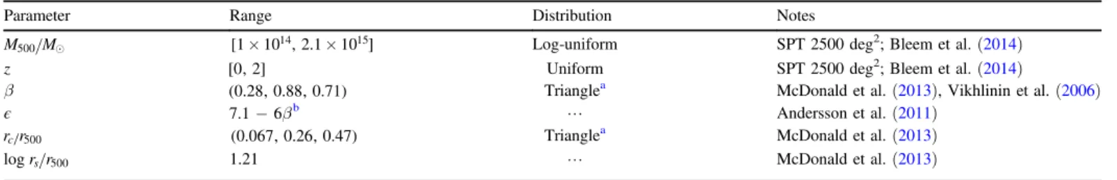
Table 1 Parameters

Parameter Range Distribution Notes



M500M [1´10 , 2.114 ´10 ]15 Log-uniform SPT 2500 deg2; Bleem et al.(2014)

z [0, 2] Uniform SPT 2500 deg2; Bleem et al.(2014)

β (0.28, 0.88, 0.71) Trianglea McDonald et al.(2013), Vikhlinin et al. (2006)

ϵ 7.1-6bb L Andersson et al.(2011)

r rc 500 (0.067, 0.26, 0.47) Trianglea McDonald et al.(2013)

r r

log s 500 1.21 L McDonald et al.(2013)

Note. All radii are in units of Kiloparsecs. We report s1 uncertainties. a

Weﬁt triangle distributions to the empirical distributions derived from McDonald et al. (2013) to avoid the long Gaussian tails that lead to unphysical clusters. We

report the(min, max, mode) of the distribution in the range column. b

The mock SZ signal is virtuallyϵ-independent. We choose ϵ to letdlogP dlogr= -0.90 at large radii, as given by the universal temperature proﬁle of Arnaud et al.(2010).

(4)

The above methods were used to generate 200 × 15 mock clusters which ranged from pure non-cool core a = 0 to strong cool core a = 3.5. We chose the maximum value a = 3.5 as even strong cool core clusters like Phoenix have a < 3.5.

2.2. Model Validation

Additional quantities were derived to demonstrate how the wide range of observed cluster properties are captured by our methodology.

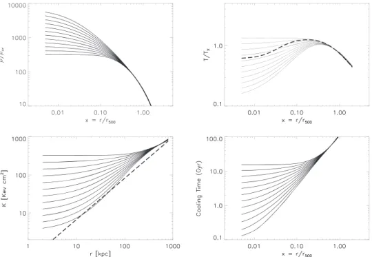
1. Temperature. Our derived temperature proﬁles are displayed in Figure 1(b). The cool core proﬁles exhibit

a central temperature drop similar to the average cool core proﬁles observed in X-ray selected samples (Vikhlinin et al. 2006). The characteristic temperatures

of our clusters range from ~1 to ~30 keV, which is in agreement with observations of massive clusters. Further-more, Tmin T0, which corresponds to the ratio of the

central cool core core temperature to the a = 0 central temperature, range from 0.1 to 0.85 in the (Vikhlinin et al.2006) clusters, which is completely covered by our

simulated clusters. Similarly, our simulations cover the range of temperature proﬁles observed in (McDonald et al.2014), which ﬁnd that the fractional temperature in

the inner 0.04R500 is Tcore T500=0.74-0.04

0.09 _{for high}

redshift, cool core clusters and higher for low redshift cool core clusters.

2. Entropy Parameter. The entropy proﬁles of our mock clusters are derived in an effort to show their resemblance to observed clusters. Following the X-ray survey conventions, an entropy parameter Kºk TnB e-2 3 is

introduced. We plot this parameter as a function of radius in Figure 1(c). Consistent with Cavagnolo et al.

(2009), Hudson et al. (2010) and McDonald et al.

(2013), the cool core clusters have a central entropy



K0 100 keV cm2, whereas for non-cool core clusters 

K0 100 keV cm2. The slope of our entropy proﬁles outside of the core is also in reasonable agreement with the accretion shock model of Voit et al. (2005), which

represents the “baseline” entropy proﬁle of clusters if radiative and other non-gravitational processes are ignored.

3. Cooling Time. The cooling time tcoolhas been shown by

Hudson et al.(2010) to be a quantity that can be used to

segregate cool cores from non-cool cores. In Figure1(d),

=

₍

L

₎

tcool 3kT ne is plotted as a function of radius. Here,

L T Z( , ) is the cooling function given by Sutherland & Dopita(1993). Most non-cool cores have central cooling

timestcool,0 1 H0 whereas the cool core clusters have

cooling timestcool,0~1 Gyr, consistent with theﬁndings of Hudson et al.(2010).

2.3. SZ Maps

For each mock cluster, we constructed an SZ map with an angular resolution of D = 0.125 arcmin, which was con-q verted to spatial resolutionDr2D=dA( )z Dqwhere dA(z) is the

angular diameter distance to the cluster. The SZ line of sight integral was then calculated at each pixel:

ò

n s D = ìíïï îïï ü ý ïï þïï q T T dl f T n k T m c ( , ) t e B (5) e CMB sz ₂ n =æ d è çç çç +- -ö ø ÷÷÷ ÷éë +

(

)

ùû f T Xe e X T ( , ) 1 1 4 1 , (6) X X sz sz

whereXºhn k TB CMB, st is the Thomson cross section, meis

the mass of the electron, c is the speed of light, and dszis the Figure 1. Clockwise from the upper left: density, temperature (Tx=òn T dV2 òn dV2 ), cooling time, and entropy as a function of cluster radius for a typical mock

cluster. All of the displayed proﬁles were obtained by cloning a single non-cool core core cluster and adding density perturbations. These plots represent 1/200th of the total dataset. In the upper right plot, the thick dashed line represent the universal temperature proﬁle of Vikhlinin et al. (2006). In the lower left plot, the thick dashed

(5)

relativistic correction as given by Itoh et al. (1998). For our

purposes, it sufﬁced to evaluate d Tsz( ) at T r(500). We made

simulated SZ maps at 97.6 and 152.9 GHz, corresponding to the effective frequency of the SPT observing bands used for cluster-ﬁnding (Carlstrom et al. 2011). Our mock SZ maps

were generated at a resolution 1 and then later convolved¢ with the SPT beam which has an effective FWHM of~ ¢1.2.

The mock SZ maps were then spatially filtered in a way identical to the SPT cluster-finding algorithm used in Reichardt et al. (2013). A multi-frequency matched spatial filter

(Haehnelt & Tegmark 1996; Melin et al. 2006) was applied

to the SZ maps in Fourier space, which accounted for the cluster gas profile, and the other sources of astrophysical signal and instrumental noise expected in the SPT maps. The spatially filtered signal at the true cluster position was then re-normalized so that it was equivalent to the unbiased SPT significance, ζ, used in Vanderlinde et al. (2010), which would

effectively correspond to the signal-to-noise of cluster in a SPT map.

These SZ maps were run through the SPT cluster-ﬁnding pipeline, which adds noise in the form of point sources and CMB anisotropy maps, before attempting to detect clusters. For each cluster, the SPT pipeline then reported ζ, the “unbiased signiﬁcance” (see Vanderlinde et al.2010; Benson et al.2011)

that roughly corresponds to the cluster signal-to-noise ratio.

2.4. Active Galactic Nuclei

In order to test the effects of including radio-loud AGNs, we created mock clusters with the following grid of parameters:

1. M500 2 ´1014M=10 , 100 1 2, 101;

2.z=0.3, 0.4, 0.5, 0.7, 1.1, 1.4, 1.7;

and we include a radio-loud AGN at the cluster center, with a range of luminosities:

3.logL1.4=23–29, DlogL1.4=1.0,

where L1.4is the 1.4 GHz luminosity inWHz-1. All other

parameters are set to their median values. The range in L

log 1.4covers the most luminous BCG in the 152 X-ray

BCG sample of Sun (2009), allowing for unusually

shallow spectrum systems that would generate a large bias.

We convert these luminosities to the SPT observing frequencies by assuming a spectral slope of a = 0.89s , where

ﬂux scales with nas_{. This slope was the median spectrum}

between 1.4 and 30 GHz for radio galaxies in a sample of 45 massive clusters observed by Sayers et al.(2012), however it is

always possible to reinterpret the results for different choices slopes. We discuss deviations from this assumption in Section 3.1. As a control, a point source is not added to one cool-core/non-cool core cluster at each mass and redshift.

3. RESULTS

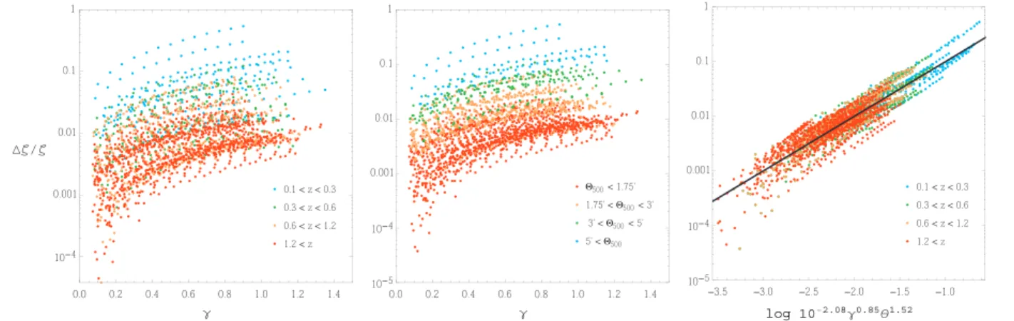
In Figure 2, we show the fractional change in the SPT detection significance as a function of the cool core cuspiness (Vikhlinin et al.2007), angular size (Q500º r500 dA( )z), and redshift. At Q500< ¢3, the SPT detection significance changes byDz z=(zCC-zNCC) zNCC0.1for any type of cool core at any redshift. The cool core bias is most pronounced for low-redshift, high mass systems, where the angular size of the SPT beam is much smaller than the angular size of the cluster so that the inner pressure profile becomes important. In principle, the resulting redshift-dependence in the bias might lead to a ~2% bias toward cool core clusters fromz~1.5 toz~0.3 in the observed cool core fractionCCFºNcool core Nclustersevolution,

but these effects should be negligible when compared to the ~30% evolution in CCF reported in e.g., McDonald et al.(2013).

In real observational studies it may be difficult to determine the density shape parameter α, as this requires a multi-parameterfit to the n np e profile and assumptions on the shape

of the cool core/non-cool core proﬁles. To ameliorate the situation, we calculate the “cuspiness” parameter gº -d logr dlogr∣r=0.04r500 (Vikhlinin et al. 2007) of all

simulated clusters. Since this quantity does not refer to the details of our parameterizations, it serves as a model-independent indicator of cool core strength; correlations between these quantities and Dz z are shown in Figure 2. The bias is well-captured by the following relation:

dz z = Dg æ è çç çç Q ö ø ÷÷÷ ÷÷ -   

( )

z 10 ( ) arcmin (7) 2.08 0.01 0.85 0.01 500 1.52 0.02

where D =g g-g∣a=0 »g-0.1. This expression gives a Figure 2. Dependence of the SZ bias on the cuspiness (g º -d r

d r

log

log ), redshift (z), and angular size (Q500º r500dA( )z) for 3000 mock clusters. In the left panel, the point color corresponds to redshift of the mock cluster. In the central panel, we color by the angular size of the cluster. The clear separation into colored bands in this plot suggests that the bias is more fundamentally tied to the angular size than it is to the redshift. In the right-most panel, we show the edge-on projection of the best-fit three-dimensional plane(Equation (7)). The ∼0.5 dex scatter is primarily due to variations in the cluster gas density profile, and the imperfect classification of cool

core strength based on theγ parameter.

(6)

practical method for estimating the SZ bias of a given cool core cluster, assuming thatz>0.1.

3.1. Radio Bias

Assuming a typical spectral slope of a = 0.89s (Sayers

et al. 2012), only sources with logL1.4>26 result in z z

D 

∣ ∣ 10% forz>0.3 andM >3 ´1014_{. Consequently,}

none of the 152 radio-loud AGNs listed in Sun(2009) would

produce a bias in excess of 10% if located in massive clusters. More generally, the radio-loud point source bias can be readily estimated by the following ﬁt to our mock clusters (see Section 2.4): dz z = - æ n è ççç öø÷÷÷ æ è çç ç ö ø ÷÷÷ ÷ æ è çç çç ö ø ÷÷÷ ÷÷ a - - S M M 0.03 1.4 GHz mJy 10 . (8) SZ 1.4 500 14 1 s

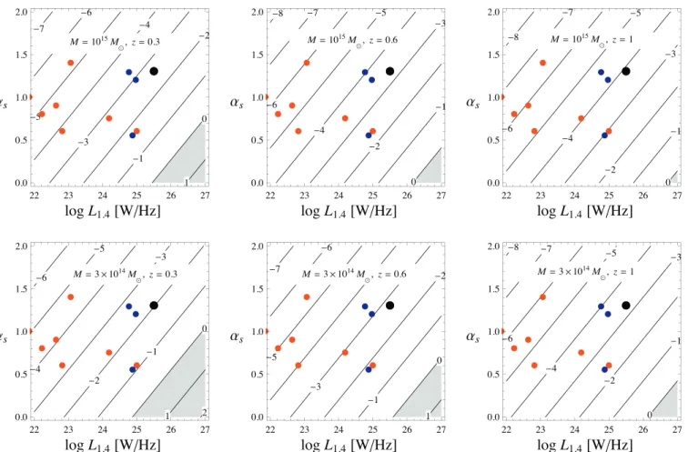
In Figure 3 we show a contour plot of Dz z on a

Q500(M500, ),z ,L1.4 parameter space. We display ﬂux and

luminosity data from a sample of X-ray selected massive elliptical galaxies from Dunn et al.(2010) and extreme AGNs

hosted in massive clusters Hlavacek-Larrondo et al.(2012). As

can be seen by Figure 3, the fractional change in SPT signiﬁcance will be strongly dependent on the assumed value of as, which has a fairly large scatter. For example, Coble et al.

(2007) measures a median value of a = 0.72s between 1.4 and

28.5 GHz. Lin et al. (2009) explicitly measure the radio

emission at frequencies ranging from 1.4 to 43 GHz in an X-ray selected sample of clusters and find mostly steep spectra (a > 0.5s ), but also find a substantial number of flat or even

inverted spectra. Neither of these studies—or any published studies of radio galaxies in clusters, for that matter—extend to ∼100 GHz, so there is still substantial uncertainty in the value of asthat we should be using.

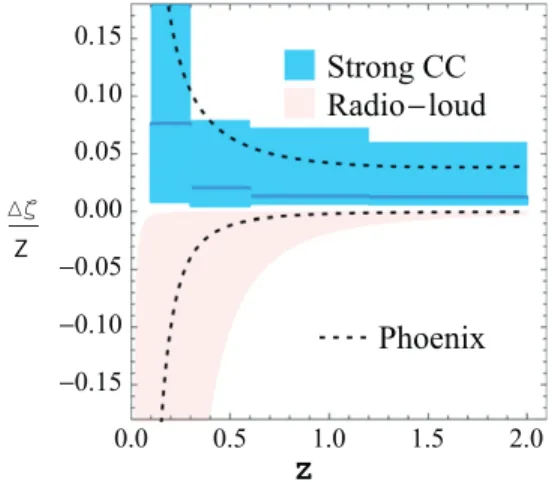
In Figure4 we show the strong cool core(a =2.75) bias and the radio-loud AGN bias as a function of redshift. Interestingly, while SZ surveys are biased toward cool cores, they are biased against radio-loud AGNs, and this bias is of the same order of magnitude as the strong cool core bias, deﬁned as the average Dz z over cool cores with a = 2.75. Since powerful radio galaxies tend to live in the center of strongly-cooling galaxy clusters, the net bias is partially canceled (see Figure4). In principle, low-redshift galaxy clusters that harbor

a powerful, radio galaxy(logL1.4 25) but lack a cool core will be under-represented in SZ surveys. However in practice, such systems appear to be uncommon in nature (see e.g., Sun2009; Dunn et al.2010). The AGN bias is more strongly

redshift dependent than the cool core bias due to the ~1 dL 2

ﬂux dimming where dLis the luminosity distance, whereas the

evolution in the simulated cool core bias is a result of SPT beam effects and weak dependencies of our parameterizations on r zcr( ).

Figure 3. Dependency of z zD on M500, redshift, radio luminosity, and spectral slope. The contours represent lines of constantlog (Dz z). If an AGN exists in the shaded region, it will overpower the SZ signal. The large black dot represents a Phoenix-like cluster at multiple redshifts. Even at z= 0.3, a Phoenix-like cluster will exhibit only a 1% bias. The most extreme systems exhibit a ~10% bias atz~0.3. Red dots represent a sample of X-ray selected massive elliptical galaxies from Dunn et al.(2010) and blue dots represent extreme AGNs hosted in massive clusters Hlavacek-Larrondo et al. (2012).

(7)

4. ROBUSTNESS OF SIMULATIONS

In this section we estimate how relaxing several of our simplifying assumptions could change our bias estimates. Though a thorough treatment of each of these issues is beyond the scope of this paper (and should be addressed by, e.g., N-body simulations), an estimate on the relative importance of these effects can be obtained by recasting these effects into an M500dependence.

4.1. Deviations from Hydrostatic Equilibrium and Non-thermal Pressure

In the absence of complicated astrophysics, a galaxy cluster will equilibrate on dynamical timescales

r

~ ~ - ~

tdynamic R500 v (G ) 1 2 109yr. For hydrostatic equili-brium to generically hold, the cooling timescale should be much longer than the dynamical timescale tcooltdynamic so

that hydrostatic equilibrium will be restored efﬁciently when gas cools. If the cooling timescale is shorter than the equilibrium timescale in the core of the cluster, we would expect pressure to be lower than what is required to maintain hydrostatic equilibrium, since gas must be sinking toward the core. This would mean that the bias should be generically lower than what we have derived, since the observed change in pressure should be smaller than that required to maintain hydrostatic equilibrium dPobs⩽dPeq.

Throughout our discussion, we have assume that pressure is purely thermal, e.g., P=nkT . Analytic work (Shi & Komatsu 2014), numerical simulations (Dolag et al. 2005; Sembolini et al.2013; Battaglia et al.2012; Nelson et al.2014),

and multi-wavelength observations (Ade & Aghanim 2013; Donahue et al. 2014; von der Linden et al. 2014; Sereno et al. 2014), however, have shown that non-thermal pressure

can contribute signiﬁcantly (~20%; increasing with cluster radius), which can lead to an underestimate of M500by about

~10% (Shi & Komatsu 2014). Sources of non-thermal

pressure include turbulence from intracluster shocks, magnetic ﬁelds, and cosmic rays. If turbulence dominates the

non-thermal pressure, non-non-thermal pressure will persist for on roughly the dynamical timescale(Shi & Komatsu2014).

From Equation(8) we see that bias scales as M1 , so toﬁrst order, we expect that adding non-thermal pressure will rescale the bias by (1+Pnon therm- Ptherm)-1, if we assume that the processes responsible for forming cool cores and providing non-thermal pressure are uncorrelated. As clusters evolve, this term could introduce an additional redshift dependence on the cool core bias, if the processes generating non-thermal pressure evolve with redshift.

4.2. Varying f_gas

Throughout this work, we have assumed that fgas =0.125 with no scatter. However, the numerical simulations of Battaglia et al. (2014b) which included radiative physics and

AGN feedback estimate a scatter ~10% in fgas at r<r500.

Eckert et al.(2013) suggest that cool core clusters and non-cool

core clusters differ in fgas by a few percent, with cool core

clusters more reliably tracing the cosmic baryon fraction. For aﬁxed number of baryons, a lower f_gaswill result in an increase in the pressure normalization, in order to overcome the steeper potential due to additional dark matter. For a cluster in hydrostatic equilibrium, kTµM r giving

µ ~

P M2 3 (1 f ) M

gas 2 3 baryon2 3 , which means that the effects

of changing1 fgaswill be roughly equivalent to changing M500.

Equations (7) and (8) can therefore be rescaled by a factor

f

(_gas 0.125). Adding intrinsic scatter in f_gaswould then simply add scatter in the SZ bias. If fgasvaried with redshift, this could

lead to a further evolutionary factor in Equation(8). However,

Battaglia et al.(2013) found little evidence for such a redshift

dependence, as has long been assumed(White et al.1993).

4.3. Effects and Evolution of AGNs

We purposefully exclude any evolution in AGN properties as a function of cluster mass and redshift, despite evidence that such links exist (e.g., Ma et al. 2013). However, by casting

Equation(8) in terms of the cluster mass, redshift, and radio

luminosity, we allow the direct incorporation of such trends into the bias estimate. By fully sampling a grid of parameters (see Section 2.4), we make certain that, regardless of how

AGNs evolve, we understand how they inﬂuence the SZ signal at all redshifts and cluster masses.

Radio-mode AGN feedback can modify the gas distribution of galaxy clusters as gas is heated and expelled from the core, leading to deviations from hydrostatic equilibrium in the inner region. Such processes will typically result in less pressure than predicted by hydrostatic equilibrium, since the gas is supported by feedback in addition to thermal pressure.

5. APPLICATION TO WELL-KNOWN SYSTEMS Using Equations (7) and (8), we can now calculate how

biased SZ surveys are (or are not) for some well-studied extreme systems. First, we consider two of the strongest known cool cores: Abell 1835 (g = 0.85, M500~ 1015 M ; McNa-

mara et al. 2006) and the Phoenix cluster (g = 1.29,

~ ´

M500 1.3 1015 M; McDonald et al. 2012). Assuming

both of these clusters are at z= 0.6, we ﬁnd z zD = 3.6% and 5.9%, for Abell 1835 and Phoenix, respectively. At z = 1.0, these biases are reduced to 2.8 and 4.2% (see also Figure4).

Figure 4. Strong cool core a =( 2.75) bias and radio-loud AGN bias. The black, dotted lines represent the massive cool core “Phoenix” cluster, with radio spectral slope a =s 1.3(McDonald et al.2014) and X-ray properties given in McDonald et al.(2013), for a range of redshifts. The pink shaded

region represents a series of radio-loud AGNs with spectral slope a ⩾ 0s ,

which demonstrates the range in possible AGN bias. The dark blue lines are the median bias in each bin and the light blue regions represent2s conﬁdence intervals. In general, the cool core bias and the radio-loud AGN bias work to roughly cancel each other.

(8)

Given that these are two of the most extreme cool cores known, we expect the typical bias toward selecting cool cores in SZ surveys to be 5% at z>0.5.

Figure 3 quantiﬁes the radio bias for a variety of nearby clusters from Dunn et al.(2010) and Hlavacek-Larrondo et al.

(2012), but here we speciﬁcally look at two well-known nearby

radio-loud central galaxies: Hydra A (S1.4=40.8Jy, z = 0.055; Bîrzan et al. 2004) and Cygnus A (S1.4=1600 Jy; z = 0.056; Bîrzan et al.2004), the latter being one of the

most powerful examples of radio-mode AGN feedback known. At z = 0.6, these two clusters would be biased low in SZ signiﬁcance by 1.8 and 110%, respectively. At z = 1.0, these biases are further reduced to 0.5 and 31%. Thus, while SZ surveys may miss the most extreme radio-loud clusters, this bias is rapidly reduced with increasing redshift. In nearby X-ray-selected clusters, 1% of clusters have radio luminosities as high as Cygnus A(M. Hogan et al. 2015, in preparation), so we expect this bias to be small overall.

6. MASS BIAS IN SZ SURVEYS

To translate SZ observations to cosmological constraints, it is necessary to estimate mass distribution of an ensemble of clusters. To this end, Vanderlinde et al. (2010) and Benson

et al.(2011) have adopted ζ as a proxy for M500by assuming a

scaling relation z µ MB_{. As a consequence, the true M} 500 of

cool core clusters will be underestimated by an amount on the order of

ò

P(Q500,g dz z)á ñ Qd 500dg on average(for ~B 1) if the calibration was performed using only a sample of non-cool core clusters. In principle, this redshift-dependent bias should translate into a distorted N M z( , ); however, the log-normal intrinsic scatter in ζ given mass has been measured to be 0.21± 0.10, calibrated using X-ray observations (Benson et al.2013). Given that the Phoenix cluster has the most-cuspy

X-ray surface brightness proﬁle of the SPT clusters with Chandra X-ray follow-up (McDonald et al. 2013), which

includes ∼90 clusters, we expect the bias in ζ to represent an extreme example. Therefore, the scatter inζ given mass due to cool cores should be a factor of several below the overall scatter in ζ and its current measurement uncertainty. The uncertainty in scatter has a negligible effect on the cosmolo-gical constraints from current SZ cluster surveys(e.g., Benson et al. 2013), so the additional scatter from the effect of cool

cores will be even less signiﬁcant.

Although we have focused on the SPT SZ survey, our results should be applicable to other SZ surveys, e.g., Planck, ACT, etc. Broadly speaking, we expect less bias in a survey with lower angular resolution and greater bias in a higher-resolution survey, since convolving a wide survey beam function with a cuspy SZ signal will smooth it to a less cuspy signal.

7. CONCLUSION

Using extensive Monte Carlo simulations of galaxy clusters and mock SPT observations, we have estimated the SZ bias due to cool cores in relaxed, massive systems. By doing so, we have constrained the cosmological and astrophysical bias due to the presence of cool cores and radio-loud AGNs in SZ surveys. Weﬁnd that the bias from cool cores is no larger than ~10% for >z 0.1 systems, and for typical high redshift objects

g D

  

z r

( 1, 500 800 kpc, 1) the bias is at the percent level. Further, the presence of radio-loud sources in cool cores should reduce the overall bias, though at low redshiftsz0.3,

the bias from radio-loud point sources should dominate any cool core bias.

Our results support the long-asserted claim that an SZ-selected sample of galaxy clusters is a robust cosmological probe: though we observe a small bias in the mass estimator, the magnitude of the bias is much smaller than the typical scatter in the mass relationship.

We provide estimates of the SZ bias as a function of redshift, mass, and cuspiness, parameters that are model-independent, as well as the radio bias. One can estimate the bias of a given system easily by plugging in values to our function

z z g

D =f z r( , 500, )+g L( 1.4, ,z M500) where f z r( , 500,g) is

given by Equation (7) and g L( 1.4, ,z M500) is given by Equation(8). By quantifying the cool core bias, astrophysical

constraints on cool core properties from SZ surveys can now be more reliably interpreted. In particular, constraints on the cool core fraction from an SZ-selected dataset are only subject to a systematic bias of order one percent, a significant reduction over X-ray selection. Since there is a stringent upper limit on the redshift evolution of the cool core fraction bias, we can now confidently say that almost all observed evolution in the cool core fraction reflects genuine cool core evolution. With the arrival of results from Planck, SPT, and the Atacama Cosmology Telescope and others, SZ surveys might be ideal for studying the mysterious balance between heating and cooling.

REFERENCES

Ade, P. A. R., Aghanim, N., Arnaud, M., et al. 2011,A&A,536, A8

Allen, S. W., Evrard, A. E., & Mantz, A. B. 2011,ARA&A,49, 409

Andersson, K., Benson, B. A., Ade, P. A. R., et al. 2011,ApJ,738, 48

Arnaud, M., Pratt, G. W., Piffaretti, R., et al. 2010,A&A,517, A92

Battaglia, N., Bond, J. R., Pfrommer, C., & Sievers, J. L. 2012,ApJ,758, 74

Battaglia, N., Bond, J. R., Pfrommer, C., & Sievers, J. L. 2013,ApJ,777, 123

Battaglia, N., Bond, J. R., Pfrommer, C., & Sievers, J. L. 2014a, ApJ,

780, 189

Battaglia, N., Bond, J. R., Pfrommer, C., & Sievers, J. L. 2014b, arXiv:1405.3346

Benson, B. A., de Haan, T., Dudley, J. P., et al. 2011, arXiv:1112.5435

Benson, B. A., de Haan, T., Dudley, J. P., et al. 2013,ApJ,763, 147

Bîrzan, L., Rafferty, D. A., McNamara, B. R., Wise, M. W., & Nulsen, P. E. J. 2004,ApJ,607, 800

Blanchard, P., Bayliss, M., & McDonald, M. 2013, in American Astronomical Society Meeting Abstracts, 221, 155.01 arXiv:1305.4184

Bleem, L. E., Stalder, B., de Haan, T., et al. 2014, arXiv:1409.0850

Carlstrom, J. E., Ade, P. A. R., Aird, K. A., et al. 2011,PASP,123, 568

Cavagnolo, K. W., Donahue, M., Voit, G. M., & Sun, M. 2009,ApJS,182, 12

Coble, K., Bonamente, M., Carlstrom, J. E., et al. 2007,AJ,134, 897

Dolag, K., Vazza, F., Brunetti, G., & Tormen, G. 2005,MNRAS,364, 753

Donahue, M., Voit, G. M., Mahdavi, A., et al. 2014, arXiv:1405.7876

Dunn, R. J. H., Allen, S. W., Taylor, G. B., et al. 2010,MNRAS,404, 180

Eckert, D., Ettori, S., Molendi, S., Vazza, F., & Paltani, S. 2013, A&A,

551, A23

Eckert, D., Molendi, S., & Paltani, S. 2011, A&A,526, A79

Fabian, A. C. 1994,ARA&A,32, 277

Foley, R. J., Andersson, K., Bazin, G., et al. 2011,ApJ,731, 86

Haehnelt, M. G., & Tegmark, M. 1996,MNRAS,279, 545

Hasselﬁeld, M., Hilton, M., Marriage, T. A., et al. 2013, arXiv:1301.0816

Hlavacek-Larrondo, J., Fabian, A. C., Edge, A. C., et al. 2012, MNRAS,

421, 1360

Hudson, D. S., Mittal, R., Reiprich, T. H., et al. 2010,A&A,513, A37

Itoh, N., Kohyama, Y., & Nozawa, S. 1998,ApJ,502, 7

Krause, E., Pierpaoli, E., Dolag, K., & Borgani, S. 2012,MNRAS,419, 1766

Lin, Y.-T., Partridge, B., Pober, J. C., et al. 2009,ApJ,694, 992

Ma, C.-J., McNamara, B. R., & Nulsen, P. E. J. 2013,ApJ,763, 63

McDonald, M. 2011,ApJL,742, L35

McDonald, M., Bayliss, M., Benson, B. A., et al. 2012,Natur,488, 349

McDonald, M., Benson, B. A., Vikhlinin, A., et al. 2013, arXiv:1305.2915

(9)

McNamara, B. R., Rafferty, D. A., Bîrzan, L., et al. 2006,ApJ,648, 164

Melin, J.-B., Bartlett, J. G., & Delabrouille, J. 2006,A&A,459, 341

Menanteau, F., Hughes, J. P., Sifón, C., et al. 2012,ApJ,748, 7

Nagai, D. 2006,ApJ,650, 538

Nelson, K., Lau, E. T., & Nagai, D. 2014,ApJ,792, 25

Planck Collaboration Ade, P. A. R., Aghanim, N., et al. 2013, arXiv:1303.5076

Reichardt, C. L., Stalder, B., Bleem, L. E., et al. 2013,ApJ,763, 127

Santos, J. S., Tozzi, P., Rosati, P., & Böhringer, H. 2010,A&A,521, A64

Sayers, J., Mroczkowski, T., Czakon, N. G., et al. 2012, arXiv:1209.5129

Sembolini, F., Yepes, G., de Petris, M., et al. 2013,MNRAS,429, 323

Semler, D. R.,Šuhada, R., Aird, K. A., et al. 2012,ApJ,761, 183

Sereno, M., Ettori, S., & Moscardini, L. 2014, arXiv:1407.7869

Shaw, L. D., Holder, G. P., & Bode, P. 2008,ApJ,686, 206

Shi, X., & Komatsu, E. 2014,MNRAS,442, 521

Sun, M. 2009,ApJ,704, 1586

Sunyaev, R. A., & Zeldovich, Y. B. 1972, CoASP,4, 173

Sutherland, R. S., & Dopita, M. A. 1993,ApJS,88, 253

Vanderlinde, K., Crawford, T. M., de Haan, T., et al. 2010,ApJ,722, 1180

Vikhlinin, A., Burenin, R., Forman, W. R., et al. 2007, in Heating versus Cooling in Galaxies and Clusters of Galaxies, ed. H. Böhringer et al. (Berlin: Springer-Verlag), 48

Vikhlinin, A., Kravtsov, A., Forman, W., et al. 2006,ApJ,640, 691

Voit, G. M., Kay, S. T., & Bryan, G. L. 2005,MNRAS,364, 909

von der Linden, A., Mantz, A., Allen, S. W., et al. 2014,MNRAS,443, 1973

White, S. D. M., Navarro, J. F., Evrard, A. E., & Frenk, C. S. 1993,Natur,

366, 429