Science Arts & Métiers (SAM)
is an open access repository that collects the work of Arts et Métiers Institute of
Technology researchers and makes it freely available over the web where possible.
This is an author-deposited version published in: https://sam.ensam.eu Handle ID: .http://hdl.handle.net/10985/16655
To cite this version :
Ebrahim ROKROK, Taoufik QORIA, Antoine BRUYERE, François BRUNO, X. GUILLAUD - Effect of Using PLL-Based Grid-Forming Control on Active Power Dynamics Under Various SCR - In: IEEE IECON'19, Portugal, 2019-10-13 - n/a - 2019
Any correspondence concerning this service should be sent to the repository Administrator : [email protected]
Effect of Using PLL-Based Grid-Forming Control
on Active Power Dynamics Under Various SCR
Ebrahim Rokrok, Taoufik Qoria, Antoine Bruyere, Bruno Francois, Xavier Guillaud Univ. Lille, Arts et Metiers ParisTech, Centrale Lille, HEI,
EA 2697 - L2EP - Laboratoire d’Electrotechnique et d’Electronique de Puissance, F-59000 Lille, France
[email protected]; [email protected]; [email protected]; [email protected]; [email protected]
Abstract—This paper investigates the effect of using
phase-locked loop (PLL) on the performance of a grid-forming controlled converter. Usually, a grid-forming controlled converter operates without dedicated PLL. It is shown that in this case, the active power dominant dynamics are highly dependent to the grid short circuit ratio (SCR). In case of using PLL, the obtained results illustrate that the SCR has a negligible effect on the dynamic behavior of the system. Moreover, the power converter will not participate to the frequency regulation anymore; therefore, the converter response time can be adjusted independently to the choice of the droop control gain, which is not possible without PLL. A simple equivalent model is presented which gives a physical explanation of these features.
Keywords—active power dynamics, droop control, grid-forming control, phase locked loop, quasi-static model
I. INTRODUCTION (HEADING 1)
Towards recent developments increasing the utilization of the renewable energy sources (RESs), one can expect a nearly 100% renewable power grid [1]. Massive integration of RESs changes the generation paradigm from conventional fossil fuel-based power plants to renewable-based generation.
RESs are connected to the AC system through the power converters. Currently these converters are controlled in a way to inject the active and reactive power to an energized AC grid. Therefore, the control relies on the existence of the instantaneous voltage formed by the AC grid. This control strategy is known as grid-following control. The increasing penetration of RESs based on the grid-following control causes a major reduction of total electrical grid inertia [2]. Low-Inertia phenomenon and its undesirable effects are already remarked in several areas, such as UK and Ireland. More details about those information are published by ENTSOE [3].
In order to solve the problem of low inertia power system, new control strategies are required to emulate the inertia effect. This topic has been extensively discussed in the literature, which has led to development of the grid-forming control strategies [4]–[7]. Among these grid-gorming control solutions, the droop-based grid-forming control and virtual synchronous machine (VSM)-based grid-forming control have become more prominent. Droop-base control mimics the synchronous machine’s (SM) speed and it is an extensively accepted baseline solution [5], [8]–[10]. As a next step, emulation of SM dynamics led to the concept of VSM [2], [11]. Although in [12] the equivalence of the droop and VSM control is proved, the discussion of VSM-based grid-forming control is beyond the scope of this paper. Therefore, we have focused on the droop-based grid-forming control schemes
where, usually, the operation of existing control schemes is not dependent on the existence of a phase locked-loop (PLL). Consequently, the effect of using PLL in droop-controlled grid-forming converter has not be addressed. This paper highlights some of the interest of introducing PLL in this scheme of control.
This paper firstly explains the origin of the droop control for the grid-forming converter based on a simple equivalent quasi-static model of the system. In the next step, the performance of the grid-forming control, which is conventionally implemented without use of any PLL, is analyzed. In this case, the quasi-static model in a very simple way demonstrates that the active power dynamics of the grid-forming converter is highly dependent to the variation of the grid short circuit ratio (SCR). The validity of the quasi-static model is proved by two levels of system dynamic model including a simplified and a full model though either pole map analysis or time domain simulation. Finally, a PLL is integrated to the model. In this case, the quasi-static model simply shows that the active power dynamics of the PLL-based grid-forming converter is independent to the variation of the grid SCR. Likewise, the time domain simulation based on the full dynamic model indicated a negligible dependency to SCR variations. As another important result of this study, it has been demonstrated that the grid-forming control without using PLL will inherently impose the task of participation in frequency support. On the contrary, the use of PLL makes the load sharing capability as an optional task for the grid-forming control.
The remaining of the paper is organized as follows. Section II gives the origin of droop control for the forming converter. In section III, the performance of grid-forming control without considering the effect of PLL has been investigated. In section IV, a PLL is integrated to the model and the consequences have been studied. Section V presents a discussion on the power sharing capability of the grid-forming control either with or without using PLL. Finally, section VI concludes the paper.
II. ORIGIN OF DROOP CONTROL SCHEME FOR GRID-FORMING
CONVERTER
The scheme of studied system consists of a 2-level voltage source converter (VSC), which is connected to an AC grid at the point of common coupling (PCC) by using a transformer (Fig. 1. a). The grid forming control has already been presented in many papers. Fundamental principles are now recalled to explain the effect of using a PLL for this kind of control. A grid-forming control is based on the phase and magnitude control of the output voltage . To simplify the
analysis, is assumed to be equal to ; the modulated output voltage by the converter. The effect of this assumption is analyzed in a second step.
The single phase equivalent circuit of the system is given in Fig. 1. b. All the variables are considered in per unit. So, the transformer is only represented by its leakage inductance. It should be noted that upper case symbols stand for root mean square (RMS) values of instantaneous signals. Lower-case symbols represent instantaneous signals.
Based on this representation, it is possible to derived two modelling equations for the active power ( ) in order to design its dynamic control. By considering the voltage at the PCC, the first one is [13]:
= . sin( ) = − , (1) where and are the root mean square (RMS) values for voltages and and are the corresponding phasor angles of the voltages in radian.
It is supposed that the active power is controlled through the difference of angle between the converter voltage angle and the grid angle . Let’s assume that a PLL delivers an estimate of the phasor grid angle . Then, we can consider the control variables as:
= − . (2)
In steady state it yields:
= . (3)
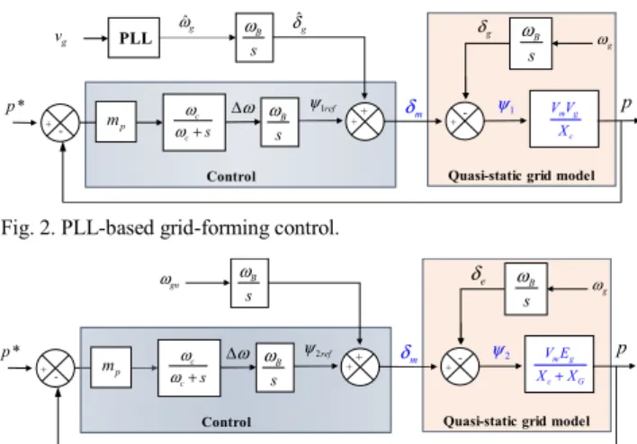
is a reference angle for the control of the power. Fig. 2 presents the grid forming control using a PLL. In this figure, the phasor angles have been replaced by the time-domain angles. In steady state, the grid angle expression is:
( ) = + ( ). (4)
The time domain converter angle is given by:
( ) = ( ) + ( ), (5)
with:
( ) = + ( ), (6)
where is the base frequency and and are the actual and estimated grid frequency, respectively. In steady state
= and = . With the time domain angles, Eq. (5)
becomes ( ) = ( ) − ( ) with ( ) = +
( ) . Therefore, it can be found that by using the time domain angles:
( ) = ( ). (7)
In steady state is constant and so, is constant. A closed loop control including an integrator is used to erase the power error in steady state (fig. 2). Hence, in steady state, the measured active power is following the reference power ∗:
= ∗. (8)
By considering the equivalent Thevenin voltage ( ) and impendance ( ) at the PCC, a second expression of the active power is:
= . sin( ) ( = − ). (9)
If the Thevenin voltage is considered as the angle reference, then = 0. Let’s introduce the time-domain angle for the voltage :
( ) = . (10)
As this equivalent Thevenin voltage is not a real voltage, a PLL cannot be used to have a precise estimate of the grid angle ( ) and so the frequency ( ). For the control design, this frequency is assumed to be equal to its nominal value . In a similar way as (5), the instantaneous converter angle is derived:
( ) = + ( ). (11)
Fig.3 illustrates the conventional droop-based grid-forming control scheme. From this figure and since ( ) = ( ) − ( ), by considering (10) and (11), it is established that the relation between and is:
( ) = − + ( ). (12)
In steady state, is constant and then is a ramp whose slope is : − . Due to the integrator in series with the gain in the control, in Laplace domain:
( ) = ∗ . (13)
Eq. (12) and Eq.(13) in time domain result in:
Δ = − . (14) p -+ e δ -+ * p ψ2 m g c G V E X+X g ω B s ω 2ref ψ c c s ω ω+ + + B s ω B s ω p m δm gn ω
Control Quasi-static grid model ω
Δ
Fig. 3. Conventional droop-based grid-forming control (without PLL).
p -+ g δ -+ * p ψ1 m g c V V X g ω B s ω 1ref ψ g v PLL ωˆg c c s ω ω + + + B s ω δˆg B s ω p m δm
Quasi-static grid model Control
ω Δ
Fig. 2. PLL-based grid-forming control. a) Scheme of the studied system.
= = =
,
= 0
b) Single-phase equivalent model of the system. Fig. 1. Presentation of the studied system.
Therefore, in steady state:
− = ( ∗− ). (15)
This last formula is equivalent to the inversed classical frequency droop control, which is also known in the literature as power synchronization control [14]. Based on this formula, is considered as a frequency droop gain. If this converter is operating in parallel with other sources, it is well known that a good load sharing when supporting frequency is linked with the choice of this droop gain. For example, the ENTSOE grid code for the generator impose a range of droop value between 1.5% and 10% [15]. Conversely, with the PLL, mp is a gain
which can be adjusted with respect to the desired closed loop dynamics.
Generally, a low-pass filter is applied to the power measurement. The aims are to filter the measurement noise, to avoid frequency jump and to decouple the dynamic of droop control loop from inner loops. Here, the filter is applied to the mismatch of the reference power and the measured power (see Fig.2 and Fig. 3) that provides the same effect [16]. The cut-off frequency of the filter has to fulfill following condition to ensure the table operation of power converter [17]:
.
20 < < .
5 , (16)
Normally, = . is chosen in the literature [16]. In this section, two control schemes have been determined from a simplified power modelling. They are compared in the next section with a much more accurate time domain model to validate the proposed model. It is then possible to explain the dynamic behavior of the system by using the literal expression of the dominant pole deduced from the simplified model. III. GRID FORMING APPROACH FOR ACTIVE POWER CONTROL
WITHOUT PLL
In this section, the dynamic of both droop control schemes is analyzed with the simplified model and it is verified with two levels of dynamic model, one neglecting the effect of the LC filter, the other which take into account the LC filter and the current and voltage loops. First, we start with the conventional grid-forming control scheme without any PLL and then, the PLL is considered.
A. Quasi-Static Model analysis
According to section II, the quasi-static model of the grid-forming converter is given in Fig.3. Since in transmission system the difference between voltage angles of adjacent
buses is supposed to be very small, therefore sin ≅ . Consequently, the whole system model in Fig. 3 is considered as linear. It is then possible to have a linear analysis of this system. The characteristic polynomial of the closed-loop system is then obtained:
Δ = + + . . . (17)
Eq. (17) reveals that the dynamic of the system is linked with , but also to the grid impedance . It means that depending on the strength of the grid the dynamics will be modified. The location of system poles is calculated by the characteristic polynomial of the closed loop transfer function that describes the dynamic behavior of the system. The natural frequency and damping ratio that give an estimation of system dominant poles are given by:
= . . . . , = . . . (18)
B. Dynamic Model presentation.
Quasi-static consideration for grid forming control of a power converter provides an estimation of the dominant pole of the system. However, to analyze the power electronic devices as the fast power components, dynamic modeling has to be developed [14].
In time domain simulation, the voltage and control loops are developed in a synchronous reference frame (SRF). The scheme of the dynamic model implementation is illustrated in Fig. 4. More information about the dynamic model of the grid-forming converter can be found in [16].
C. Validation of Quasi-Static Model
In order to verify the validity of the quasi-static model in terms of system dominant pole estimation, both quasi-static and dynamic models are implemented in Matlab-Simulink environment for time domain simulation. It should be noted that the average model of power converter is considered. Power-conservative form of Park transform [18] is used in the simulations. In Ref. [16], it is shown that the fast dynamics of inner control loops has a negligible effect on the system dominant poles so it is possible to introduce an intermediate level of model where the LC is removed.
A second way to validate the quasi static model is to compare the poles with the dynamic model. For the sake of simplicity, only the poles of the system without the LC filter are considered for this comparison. System parameters are given in Table I. Considering these values, the natural
frequency and damping ratio in static model are obtained as follows: = 20.2 / , = 0.777 .
Fig. 5 shows the system poles for both quasi-static and simplified dynamic models. It can be seen that the quasi-static model gives a good estimation of system dominant poles. Time domain simulation for has been performed for all three models. A step is applied to the power reference at t=2 s. Fig. 6 validates the simplified quasi-static and dynamic models.
D. Influence of SCR
According to IEEE definition, SCR is the ratio of the available short-circuit current, in amperes, to the load current, in amperes at a particular location [19]. At the PCC, SCR is expressed as:
= (19)
Ref. [20] has defined the grid strength as strong, weak or very weak if its SCR is greater than 3, between 2 and 3, or
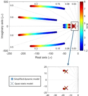
lower than 2, respectively; Fig. 8 shows the system pole map for a wide range of grid strength.
Fig. 7 indicates the pole trajectory of the studied system for both quasi-static and simplified dynamic model with respect to the SCR. It can be clearly seen that the system dominant poles are moving with respect to the SCR value and the quasi-static model gives a good estimation of the dominant poles. For the given range of 1.2 < SCR < 8, the natural frequency and damping ratio drawn from the simplified model are varying in the following range:
14.1 < < 26.8 / , 0.58 < < 1.11
Simplified dynamic model Quasi-static model
Fig. 5. Validation of quasi-static model by pole analysis. TABLE I. SYSTEM PARAMETERS OF FIG.4.
Parameter Value Parameter Value
Base power 1 GW ∗ 0.0 pu
Converter nominal power 1 GW 0.02 Base voltage 320 kV 31.4 rad/s
Grid voltage 1 pu 0.09 pu
Base frequency in rad/s 314.16 60 rad/s Grid nominal frequency 1 pu 1 pu
AC line-line voltage 320 kV 0.15 pu Transformer inductance 0.15 pu 0.066 pu Transformer resistance 0.005 pu 0.52 Grid thevenin inductance 0.333 pu 1.16
Grid thevenin resistance
= /10 0.0333 pu 0.73
640 kV 1.19
Fig. 6. Validation of quasi-static model by time domain simulation.
-250 -200 -150 -100 -50 0 Real axis ( ) -400 -300 -200 -100 0 100 200 300 400 0.8 0.5 0.3 0.15 0.08 0.03 0.8 0.5 0.3 0.15 0.08 0.03 1.2 2 3 4 5 6 7 8 -25 -20 -15 -10 -5 -30 -20 -10 0 10 20 30
Simplified dynamic model Quasi-static model
Fig. 7. Validation of quasi-static model by pole map for various SCR.
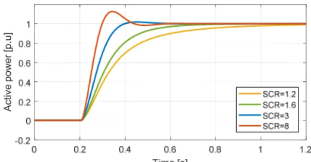
Fig.8. Effect of SCR on the active power dynamics for conventional grid-forming control.
A
ctive pow
Time domain simulation for full dynamic model of the system verifies the high dependency of the active power dynamics to the value of SCR as it is illustrated in Fig. 8.
IV. ACTIVE POWER CONTROL WITH PLL
A PLL with a 10ms response time is used to provide the grid angle estimation at the PCC. The basic block diagram of a PLL is illustrated in Fig. 9. In this case, according to the quasi-static model, the closed-loop transfer function of the system can be expressed as follows:
Δ = + + . . . (20)
The system voltages and are constant (1 pu). Due to the fact that in transmission system the voltages of adjacent buses are close to each other, in (20) can be replaced by . Therefore, the natural frequency and damping ratio
can be expressed as follows:
= . . . . , = . . . (21)
In this expression, and are supposed to be close to 1 pu. Contrary to (18), this loop dynamics does not depend on the grid impedance .
Considering the parameters of Table I and in order to have the same dominant poles presented by quasi static model as in the previous case with SCR =3, the value of has to be modified to = 0.0062.
A. Influence of SCR
Fig. 10 shows the pole trajectory of the studied system for both quasi-static and simplified dynamic model in presence of PLL. It can be seen that the dominant pole are much less
sensitive to the grid SCR. Time domain simulation using full dynamic model of the system which is presented in Fig. 11 verifies this result.
B. Influence of
The response time of the conventional grid-forming controlled converter is imposed by the droop criteria and grid SCR. Therefore, it cannot be chosen. In contrary, as previously explained in section II, can be adjusted with no effect on the frequency support in presence of PLL. Then, the active power response time of the PLL-based grid-forming controlled converter is adjustable by the parameter . Fig. 12 illustrates the effect of the parameter on the active power dynamics of PLL-based grid-forming controlled converter.
V. DISCUSSION ON POWER SHARING CAPABILITY
As already explained, the droop-based grid forming control without using PLL will inherently propose a mandatory frequency support to the grid. This requirement is
Fig.12. Effect of parameter on the active power dynamics of PLL-based grid-forming controlled converter.
0 0.1 0.2 0.3 0.4 0.5 0.6 0.7 0 0.5 1 1.2 SCR = 1.6 SCR = 3 SCR = 8 0 0.1 0.2 0.3 0.4 0.5 0.6 0.7 0 0.5 1 1.2 SCR = 1.6 SCR = 3 SCR = 8 0 0.1 0.2 0.3 0.4 0.5 0.6 0.7 Time [s] 0 0.5 1 1.2 SCR = 1.6 SCR = 3 SCR = 8 mp=0.009 mp=0.00621 mp=0.011 -250 -200 -150 -100 -50 0 Real axis ( ) -500 0 500 0.8 0.5 0.3 0.15 0.08 0.03 0.8 0.5 0.3 0.15 0.08 0.03 1.2 2 3 4 5 6 7 8
Simplified dynamic model Quasi-static model
Fig. 10. System pole map under various SCR in presence of PLL. 0 + PI − controller
Park( )
+ ++
( )
Fig. 9. Scheme of PLL.
Fig. 11. Effect of SCR on performance of the PLL based grid-forming controlled converter. A cti ve P ow er [p .u ]
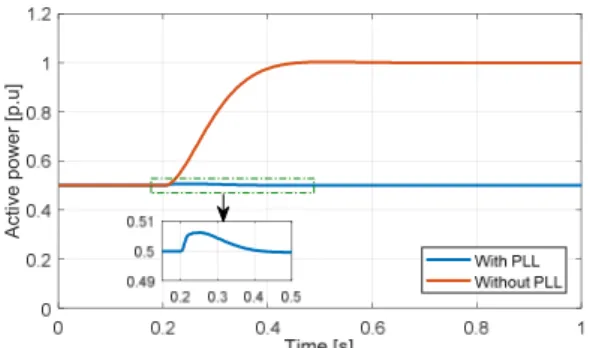
considered as a drawback for this kind of control. In contrary, the participation in frequency support is an optional choice for the PLL-based grid-forming control, which can be implemented through an outer control loop. To verify this significant result, let’s consider a drop in the grid frequency as illustrated in Fig. 13. A virtual frequency step of 0.01 pu is applied at t=2 s to the voltage source frequency passing through a first order 50 ms time constant (i.e. = 0.05 ). The droop gain = 0.02 is chosen for the case of operation without PLL. SCR is equal to 3 and to have the same system dominant poles, the parameter = 0.0062 is chosen for the case of using PLL in the control. Fig. 14 shows the result of time domain simulation for both conventional and PLL-based forming control. It can be seen that the PLL-based grid-forming controlled converter do not participate in frequency support as expected. The implementation of power sharing task for the PLL-based grid-forming control in an outer loop provides more flexibility for the converter owner. For instance, a frequency dead-band can be defined so that the converter doesn’t need to change its output power for a small frequency variation. Moreover, the maximum amount of provided frequency support can be adjusted by using a saturation action. It is not possible to obtain these facilities while the PLL is not included in the control.
VI. CONCLUSIONS
This paper represented the high significance of using the quasi-static model for the grid-forming controlled converter. It was shown that the quasi-static model simply gives a set of valuable information including an accurate location of the system dominant poles and the dependency of the converter active power dynamics to the system parameters. These kind of information, in spite of simplicity, are very useful in choosing a proper control strategy for the power converters. It was also shown that by integrating a PLL into the grid-forming control, more facilities for the power sharing capability task of the power converter is provided.
As stated in the paper, some simplification assumptions were used to derive the quasi-static model. Therefore, the validity range of the model is limited and the investigation on that can be considered as a future work.
ACKNOWLEDGMENT
This work was supported by the project “HVDC Inertia Provision” (HVDC Pro), financed by the ENERGIX program of the Research Council of Norway (RCN) with project number 268053/E2, and the industry partners; Statnett, Statoil, RTE and ELIA.
REFERENCES
[1] B. Johnson, P. Denholm, B. Kroposki, and B. Hodge, “Achieving a 100% Renewable Grid,” IEEE Power Energy Mag., pp. 61–73, 2017. [2] S. D’Arco, J. A. Suul, and O. B. Fosso, “A Virtual Synchronous
Machine implementation for distributed control of power converters in SmartGrids,” Electr. Power Syst. Res., vol. 122, pp. 180–197, 2015. [3] ENTSO-E, “High Penetration of Power Electronic Interfaced Power
Sources (HPoPEIPS),” no. March, 2017.
[4] J. G. Webster, T. Dragičević, L. Meng, F. Blaabjerg, and Y. Li, “Control of Power Converters in ac and dc Microgrids,” Wiley Encycl.
Electr. Electron. Eng., vol. 27, no. 11, pp. 1–23, 2012.
[5] T. Qoria, F. Gruson, F. Colas, X. Guillaud, M. S. Debry, and T. Prevost, “Tuning of cascaded controllers for robust grid-forming voltage source converter,” 20th Power Syst. Comput. Conf. PSCC 2018, pp. 1–7, 2018. [6] E. Rokrok, M. Shafie-khah, and J. P. S. Catalão, “Review of primary voltage and frequency control methods for inverter-based islanded microgrids with distributed generation,” Renew. Sustain. Energy Rev., vol. 82, pp. 3225–3235, 2018.
[7] A. Tayyebi, F. Dörfler, Z. Miletic, F. Kupzog, and W. Hribernik, “Grid-Forming Converters – Inevitability, Control Strategies and Challenges in Future Grids Application,” CIRED Work., 2018. [8] M. C. Chandorkar, D. M. Divan, and R. Adapa, “Control of parallel
connected inverters in standalone ac supply systems,” IEEE Trans. Ind.
Appl., vol. 29, no. 1, pp. 136–143, 1993.
[9] J. W. Simpson-Porco, F. Dörfler, and F. Bullo, “Synchronization and power sharing for droop-controlled inverters in islanded microgrids,”
Automatica, vol. 49, no. 9, pp. 2603–2611, 2013.
[10] B. Johnson, M. Rodriguez, M. Sinha, and S. Dhople, “Comparison of virtual oscillator and droop control,” 2017 IEEE 18th Work. Control
Model. Power Electron. COMPEL 2017, 2017.
[11] H. Bevrani, T. Ise, and Y. Miura, “Virtual synchronous generators: A survey and new perspectives,” Int. J. Electr. Power Energy Syst., vol. 54, pp. 244–254, 2014.
[12] S. D’Arco and J. A. Suul, “Equivalence ofVirtual Synchronous Machines and Frequency-Droops for Converter-Based MicroGrids,”
IEEE Trans. Smart Grid, vol. 5, no. 1, pp. 394–395, 2014.
[13] J. J. Grainger and W. D. Stevenson, Power system analysis. New York: McGraw-Hill, 1994.
[14] L. Zhang, L. Harnefors, and H. Nee, “Power-Synchronization Control of Grid-Connected Voltage-Source Converters,” IEEE Trans. Power
Syst., vol. 25, no. 2, pp. 809–820, 2010.
[15] “Requirements for Generators.” [Online]. Available: https://www.entsoe.eu/network_codes/rfg/. [Accessed: 20-May-2019]. [16] “H2020 Migrate-Deliverable D3.2.” [Online]. Available:
https://www.h2020-migrate.eu/. [Accessed: 21-May-2019].
[17] S. D’Arco, J. A. Suul, and O. B. Fosso, “Automatic Tuning of Cascaded Controllers for Power Converters Using Eigenvalue Parametric Sensitivities,” IEEE Trans. Ind. Appl., vol. 51, no. 2, pp. 1743–1753, 2015.
[18] P. C. Krause, O. Wasynczuk, S. D. Sudhoff, and S. Pekarek, Analysis
of Electric Machinery and Drive Systems. New York: IEEE press,
2002.
[19] IEEE Power and Energy Society, “IEEE Recommended Practice and Requirements for Harmonic Control in Electric Power Systems,” IEEE
Stand., 2014.
[20] IEEE Power Engineering Society, IEEE Guide for Planning DC Links
Terminating at AC Locations Having Low Short-Circuit Capacities.
ISBN 1-55937-936-7, 1997. Fig. 13. Implementation of a frequency step in the studied system.
Fig. 14. Result of power sharing study for both conventional and PLL-based grid-forming control.
A
cti