HAL Id: hal-01072736
https://hal.archives-ouvertes.fr/hal-01072736
Preprint submitted on 8 Oct 2014
HAL is a multi-disciplinary open access
archive for the deposit and dissemination of
sci-entific research documents, whether they are
pub-lished or not. The documents may come from
teaching and research institutions in France or
abroad, or from public or private research centers.
L’archive ouverte pluridisciplinaire HAL, est
destinée au dépôt et à la diffusion de documents
scientifiques de niveau recherche, publiés ou non,
émanant des établissements d’enseignement et de
recherche français ou étrangers, des laboratoires
publics ou privés.
EU ETS, Free Allocations and Activity Level
Thresholds. The devil lies in the details
Frédéric Branger, Jean-Pierre Ponssard, Oliver Sartor, Misato Sato
To cite this version:
Frédéric Branger, Jean-Pierre Ponssard, Oliver Sartor, Misato Sato. EU ETS, Free Allocations and
Activity Level Thresholds. The devil lies in the details. 2014. �hal-01072736�
EU ETS, FREE ALLOCATIONS AND ACTIVITY LEVEL THRESHOLDS
THE DEVIL LIES IN THE DETAILS
Frédéric BRANGER
Jean-Pierre PONSSARD
Oliver SARTOR
Misato SATO
Cahier n°
2014-23
ECOLE POLYTECHNIQUE
CENTRE NATIONAL DE LA RECHERCHE SCIENTIFIQUE
DEPARTEMENT D'ECONOMIE
Route de Saclay
91128 PALAISEAU CEDEX
(33) 1 69333033
http://www.economie.polytechnique.edu/
mailto:[email protected]
EU ETS, Free Allocations and Activity Level Thresholds
The devil lies in the details
Frédéric Branger1
, Jean-Pierre Ponssard
2, Oliver Sartor
3, Misato Sato
4October 2014
ABSTRACT
This paper investigates incentives for firms to increase output above the activity level thresholds (ALTs) in order to obtain more free allowances in the EU Emissions Trading Scheme. While ALTs were introduced in order to reduce excess free allocation to low-activity installations, for installations operating below the threshold, the financial gain from increasing output to reach the threshold may outweigh the costs. Using installation level data for 246 clinker plants, we estimate the effect of ALTs on output decisions. The ALTs induced 5.8Mt of excess clinker production in 2012 (4% of total EU output), which corresponds to 5.2Mt of excess CO
2 emissions (over 5% of total sector emissions). As
intended, ALTs do reduce overallocation (by 6.6million allowances) relative to a scenario without ALTs, but an alternative output based allocation would further reduce overallocation by 39.5million allowances (29% of total cement sector free allocation). Firms responded disproportionately to ALTs in countries with low demand, especially in Spain and Greece. The excess clinker output lead to increased EU clinker and cement exports, production shifting between plants and also an increase in clinker content of cement thus
reducing the carbon efficiency of cement production.
JEL Classification: D24, H23, L23, L61
Keywords: Activity level thresholds, EU ETS, carbon trading, free allowance allocations, cement
"
"""""""""""""""""""""""""""""""""""""""""""""""""""""""""""""
1 CIRED, [email protected]2 CNRS and Ecole Polytechnique, [email protected] 3 IDDRI, [email protected] IDDRI, [email protected]
4 London School of Economics, [email protected] (Corresponding author), postal address: LSE, Houghton Street,
1. Introduction
The justification for using free allocations in emission trading schemes has evolved over time. Historically, in schemes such as the U.S. acid rain program, it was introduced as a compensation mechanism for the owners of existing industrial assets for a change in the rules of the game (Ellerman et al., 2000). A lump sum transfer would be made to existing assets through a predetermined amount of annual free allocations for a given number of years. The free allocations offset the costs to purchase pollution permits on the market.
Such methods are termed “grandfathering”, “historic”, “lump-sum” or “ex-ante” allocation.5
New assets would not be allowed free allocations and thus would have to pay the full permit price on the market. As long as the free allocations are predetermined, all assets (old and new) would compete on the same playing field, the price of permits would provide the same opportunity cost for mitigating pollution, and in theory, the output price of the goods sold would incorporate the price signal for consumers.
More recently, free allocations have been explicitly used (or have been proposed to be used) as a way to strategically alleviate the risk of offshoring production and emissions (so-called “carbon leakage”) for Energy-Intensive and Trade-Exposed (EITE) sectors such as cement, chemicals and steel. In the absence of border carbon adjustment, the implementation of which is considered as politically difficult, economic theory suggests that “output-based” allocation (OBA) should be used (e.g. Fischer and Fox 2007, Quirion 2009, Fischer and Fox 2012, Meunier et al 2012). Indeed an OBA scheme has been implemented within the Californian ETS which began in 2012 (California Air Resources Board, 2013). In contrast the
EU ETS Phase 3 is unique in using a complex system. It combines an ex-ante calculation6 of
an allocation and subsequent lump-sum transfer based on historic output (and multiplied by an emissions intensity benchmark) with a possible ex-post calculation and adjustment of this lump-sum according to rules related to actual capacity and activity levels as defined in Decision (2011/278/EU) (European Commission, 2011). Situations in which ex-post adjustments occur include the arrival of new entrants into the market, plant capacity extension/reduction, plant closure and partial cessation or recommencement of activity at
an existing plant. These latter rules are governed by the activity level thresholds (ALT)7.
Qualitatively, ETS schemes with ALT approximate OBA: the amount of free allocations will
vary with the activity level, and the overallocation profits8 associated with ex-ante schemes
will be reduced.9 The advantage of ALT rules is that they allow for a fixed cap (in fact a cap
which will not exceed a predetermined amount for existing installations and the reserve for new entrants). One disadvantage is that they introduce an element of complexity in the scheme. Under these non-linear rules, the lump sum transfer of allowances to EITE sectors is reduced by 50%, 75% or 100% if the annual level of production of the plant falls below 50%, 25% or 10% respectively, of the historical activity level (HAL) of production that is used to determine the ex-ante allocation (European Commission, 2011).
"""""""""""""""""""""""""""""""""""""""""""""""""""""""""""""
5 The term ”grandfathering” is usually used in a narrow sense, whereby allocation is based purely on past emissions
or output, whereas the other terms tend to also incorporate allocation methods such as the EU ETS Phase 3 rules, which is based on past production but is also multiplied by a benchmark.
6 Note that ex-ante and ex-post refer to whether the calculation of the freely allocated amount of allowances occurs
prior to or following the production and emissions for which allowances are to be allocated.
7 New entrant provision and closing rules were already in place in Phases 1 and 2 of the EU-ETS. A closure rule is
also used in the Californian ETS.
8 Overallocation profits can be distinguished from windfall profits, which refer to the profits from free allocation
where emitters additionally profit from passing on the marginal CO2 opportunity cost to product prices, despite receiving the allowances for free. Overallocation profits can occur even in the absence of cost pass through, if output fall short of historic levels.
9 Windfall and overallocation gains have been a persistent shortcoming of the use of ex-ante free-allocation
A second disadvantage is that the ALTs introduce distortions, which is the focus of this paper. A recent study on the EU ETS impacts on the cement sector 2005-2013 (Neuhoff et al.,
2014)10 found preliminary evidence through data analysis and comprehensive interviews
with industry executives, that new ALTs introduced in 2013 provided cement installations the incentive to adjust output levels. The rationale is as follows. Since the free allocation in year t+1 is directly linked to output in year t, if output levels lie below the threshold levels, there may be an incentive to increase output in year t to achieve the relevant threshold (.10, .25, .50) and receive higher free allocations in year t+1. In this paper, such strategic adjustments of output motivated by ALTs is termed “gaming” behaviour, in line with the management literature (e.g. Jensen, 2001). Neuhoff et al. (2014) report that in interviews, company executives consistently confirm these practices where the regional cement market demand is insufficient to reach the minimum activity level. They identify three channels to marginally increase production in a plant which is producing below the threshold:
• Production shifting among local plants, i.e. reducing the production at a plant which
is well above the threshold to increase the production at the plant which is below;
this generates some transport costs11 so that it can be too costly to be undertaken at
a large scale;
• Exports of clinker to other markets so as not to perturb the local market while
increasing production; this generates some cost in terms of export price rebate, since these exports would not naturally occur;
• Increase the clinker to cement ratio, i.e. incorporate within limits more clinker in
cement instead of using less costly cementitious additives such as slag of flying ashes; this directly generates some cost.
The objective of the paper is to quantify the magnitude of these distortions, and discuss whether the disadvantages of ALTs balance the advantages.
Empirical studies on this subject remain limited. Most of these studies have examined the distortive effects of combined ex-ante allocations with ex-post new entrant and plant closure provisions. Pahle et al. (2011), Ellerman (2008) and Neuhoff et al. (2006) compared the new entrant provision relative to auctioning. These papers argued that new entrant provisions distort via their impact on investment decisions (essentially by acting as a subsidy). Meunier et al. (2014) compared this same provision with an output-based scheme whenever firms face an uncertain demand. They showed the entrant provision could induce excessive new investments in the EU cement sector. Fowlie et al. (2012) compare ex-ante schemes with closure rules with an output-based scheme and show that the lifetime of old inefficient plants would be unduly extended with the former. None of these studies has discussed the impacts of the possible distortions associated with the addition of “non-linear” ex-post adjustments to ex-ante allocation via the use of ALTs, such as introduced in the EU ETS Phase 3 (2013-2020).
While our analysis only concerns the cement sector, and has been done in a context of low carbon price, we think that its relevance may go beyond the sector context, and it could be potentially relevant to other EITEs. Altogether, we argue that the benefits of implementing
"""""""""""""""""""""""""""""""""""""""""""""""""""""""""""""
10 Three co-authors of this paper participated in this study and in conducting interviews that were carried out. 11 McKinsey (2008) estimate that transport costs for a tonne of clinker from Alexandria to Rotterdam are roughly
€20/tonne, and that inland shipping costs are approximately €3.5/tonne per 100km and inland road transport was about 8.6€/ton per 100km.
ALTs in terms of reduced overallocation profits does not outweigh the significant costs in the form of distortions, hence ALTs should be abandoned.
The paper is organized as follows. Section 2 discusses the EU ETS Phase 3 allocation rules, the predicted gaming behaviour from thresholds and the alternative allocation rules. Section 3 describes our conceptual framework for evaluating the effects of ALTs, the methodology, data sources, as well as the key assumptions involved in our analysis. Section 4 presents the results. Section 5 concludes and discusses some policy recommendations.
2. ETS free allocation rules and gaming of ALTs
2.1. The EU-ETS Phase 3 free allocation rules
In Phase 3 of the EU ETS, installations in sectors “deemed to be exposed to carbon leakage” are eligible to receive free allocation of emission allowances. The determination of the free allowances for each installation combines an ex-ante calculation, based on the historic
output for existing installations (known as the “historical activity level” or “HAL”12) or the
initial capacity for new installations, with an ex-post calculation based on the ongoing activity level of this installation as defined in Decision (2011/278/EU) (European Commission, 2011). The ex-post calculation provides step wise adjustments intended to reflect changes in market volumes. These adjustments follow complex procedures.
For existing installations, the precise relationship that determines the next-period allocation from ex-ante and ex-post values is summarised by Equations 1 and 2 below. The amount of
free allocations to an installation, i, at period t+1, for an eligible product, p is denoted Ai,p,t+1 .
A
i,p,t+1 = CSCFt x Bp x HALi,p x ALCFt+1(qi,p,t/HALi,p), (1)
In equation (1) CSCF
t is the uniform cross-sectoral correction factor
13, B
p is the benchmark
for product p, 14 HAL
i,p represents the historical activity level,qi,p,t represents the output of
the eligible product in year t; and ALCF(qi,p,t/HALi,p) is the activity level correction factor. The
latter factor defines a step wise function for the thresholds. It is defined as:
!"#$!!! !"#!! = ! 1,!!!!!!!!!!!!!!!!≥ 0.5!!"#!!!!!!!!!!!!!!! 0.5,!!!!!!!0.25!!"# ≤ ! !!< 0.5!!"# 0.25,!!!!!!0.10!!!"# ≤ !!< 0.25!!"#! 0,!!!!!!!!0!!"# ≤ !!< 0.10!!"# !!!!!!!!!!!!!!!!!!!!!!!!!!!!!!!!!!!!!!!!!!!!!!!(2)
For new installations, the historic activity level is replaced by the capacity, to be precisely
determined according to the rules.15
2.2. Gaming and thresholds
Gaming behaviour refers to artificially increasing production to attain thresholds, in order to obtain more allowances. Consider a plant for which the “business as usual” activity level for year 2012 would be at say 40% of its historic activity level. Increasing production up to 50% of its historic activity level allows doubling the free allocation received. A rough
"""""""""""""""""""""""""""""""""""""""""""""""""""""""""""""
12 The benchmarked product-related historical activity level (HAL) is defined as maximum of the median annual
historical production of the product in the installation (or sub-installation) concerned during either 2005-2008 or 2009-2010. (cf. Decision (2011/278/EU)).
13 This is determined by comparing the sum of preliminary total annual amounts of emission allowances allocated
free to installations (not electricity) for each year over the period 2013-2020. In 2013 the CSCF is equal to 0.9427, then declines at 1.74% per year.
14 Product benchmarks in general reflect the average performance of the 10% most efficient installations in the
sector or subsector in the years 2007-2008. The benchmarks are calculated for products rather than inputs Decision (2011/278/EU).
calculation with a clinker plant illustrates the potential benefit of gaming. Suppose HAL refers to 1 Mt/year, the business as usual is 0.4 tons so that the plant needs to increase production by 0.1 tons to achieve the 50% threshold. At 9 €/t CO
2 in 2013, if the firm gets
100% of free allowances relative to HAL it is worth 6.5 M€; losing 50% allowances implies a
loss of 3.25 M€. Suppose the emission intensity is say 0.8 t CO2/t of clinker. The increase in
emissions is then equal to 0.080 t CO
2 which at 9 €/t CO2 amounts to 0.72 M€.
In the presence of activity level thresholds, the net benefit of gaming in terms of allocations is the difference between the increased free allocations and the certificates needed to cover the increased production (in our case 2.53M€=3.25M€-0.72M€). The net benefit depends on
the price of CO2, the benefit rising with the price. However, this artificial increase of
production involves cost inefficiencies, which can be assumed increasing function of the
extra production, independent of the CO2 price but dependent on the plant. These cost
inefficiencies can up to a point cancel out the gains from increased free allocation. This is shown in Figure 1, where gaming is undertaken only if the increased production to attain
the threshold is less than ∆!!. In our case, if the extra production of 0.1 ton of clinker does
not involve cost inefficiencies of more than 2.53M€, gaming is profitable.
Figure 1: The value of gaming. The installation engages in gaming when ∆! < ∆!!. ! refers to the
carbon intensity of the plant. Benefits are increased free allocations minus extra emissions.
Evidence of strong responses to thresholds – where small changes in behaviours lead to large changes in outcomes – has been found in the recent literature. Sallee and Slemrod (2012) find evidence that the automakers respond to notches in the Gase Guzzler tax and to mandatory fuel economy labels by manipulating fuel economy ratings in order to qualify for more favourable treatment. The management control literature also finds that managers tend to react strongly to the existence of a threshold. This is the case, for example, when bonuses depend on the achievement of a given level of sales for a sales manager, a given productivity indicator for a plant manager, a given return on investment for a business manager, a given level of the total shareholder return for a CEO, etc (Locke 2001). In a well-known article, Jensen (2001) points out that such “gaming” behaviour is perfectly rational under threshold rules. He argues that these rules imply an agency cost which is largely underestimated and suggests that linear bonus schemes should be preferable.
2.3. Alternative free allocation rules
The EU ETS Phase 3 rules can be compared with an ex ante allocation without ALTs similar
to Phase 1 and 216 or an output-based allocation scheme. Under OBA, the next period
allocation is determined according to an equation similar to equation (1) (with !!,!,!⟷
!"#!,!×!"#$(!!,!,! !"#!,!)). The scheme therefore has no thresholds, and the historic activity
level HAL is replaced by the previous year activity level !! so as allocations are altered on a
continuous yearly production basis. In this paper, we will evaluate the impact of the ALTs by contrasting four scenarios, with their respective acronym:
( Ex-ante free allocation with ALTs (Phase 3 allocation rules) and gaming (EXALTG)
( Ex-ante free allocation with ALTs (Phase 3 allocation rules) without gaming
(EXALTNG)
( Ex-ante free allocation without ALTs (Phase 1&2 allocation rules) (EX)
( Ex-post output based allocation (OBA)
Scenario EXALTG corresponds to what was observed in Phase 3. Scenario EXALTNG applies the same rules but it is a hypothetical scenario where no gaming behaviour is observed. Therefore EXALTNG, EX and OBA all represent counterfactuals.
3. Methodology and data
3.1. Conceptual framework
Since 2013 is the first year the threshold rule is in place, the 2012 activity level will directly determine the allocation allowances for 2013. Our analysis therefore focuses on outcomes of installations in the EU ETS in 2012.
The preliminary results in Neuhoff et al (2014) provided evidence of distortions due to the thresholds, based on interviews with industry executives and comparison between 2011 and 2012 data. The present study will attempt to quantify such distortions. This necessitates the elaboration of a counterfactual scenario for 2012 (what would have happened had the threshold rule not been implemented). A simple comparison between 2011 and 2012 would give inaccurate results because of underlying market trends e.g. cement consumption fell by 13% at the EU level between 2011 and 2012. Comparing with a counterfactual enables us to understand the magnitude of the excess output due to ALTs, and the corresponding excess emissions and overallocation profits. A straightforward caveat is that our results are then very dependent on the counterfactual. This is why it is constructed using a method as robust and unbiased as possible, based on historical data and econometrics (see Appendix C).
3.2. The cement sector
Our analysis focuses on the cement sector to investigate the magnitude of distortions arising from ALTs for three reasons. First, it ranks amongst the highest in terms of carbon intensity per value added thus, the effects of free allocation rules are magnified. Second, unlike chemicals and steel with many product categories and differentiated impacts, the cement sector is characterised by relatively homogeneous products and production processes. Thus inferring production (activity) from emissions is more straightforward (see further). Third, as the sector experienced a demand collapse in the order of 50% or more between 2007 and 2012 in several member states (Boyer and Ponssard, 2013), the ALT rules were likely to have been more a relevant factor for operational decisions during the period of investigation.
"""""""""""""""""""""""""""""""""""""""""""""""""""""""""""""
The cement production process can be divided into two basic stages: production of clinker from raw materials and the subsequent transformation of clinker into cement by grinding with other mineral components. Clinker production accounts for the bulk of carbon emissions in cement production, and the reduction of the clinker-to-cement ratio is one of the most efficient ways of mitigation in the sector. Further, allocation under the EU ETS is
based on a benchmark on clinker rather than cement or hybrid benchmark17.
3.3. Distinguishing between installations above and below thresholds
As described in Section 2.1, allocation is determined by q/HAL, however, data on installation activity levels (i.e. clinker output) are not publicly available. However, it is possible to infer clinker plants’ activity levels inferred from plant level emissions data, which are available from the European Union Transactions Log (EUTL). That is, it is possible to use the observed ratio of publically-reported verified emissions (E) relative to the Historical Emissions Level (HEL), to proxy the share of unobserved activity level relative to Historical Activity Level
(HAL) i.e. E/HEL ≈ q/HAL.18 This approximation is possible owing to the very strong and
direct relationship between production of clinker, a highly homogeneous product, and emissions. Indeed the emissions intensities of clinker production have changed only very marginally in the EU in recent years between 2005 and 2012 (GNR Database).
However, in distinguish between installations that are above or below thresholds (25% and 50% of q/HAL), an element of uncertainty is introduced due to the approximation of plant activity level based on emissions data. As detailed in A1., we ensure that installations are correctly identified using 2013 allocations data. This reveals whether or not the installation had seen its allocation reduced because of 2012 activity levels. 2013 allocation data also allowed us to obtain clinker carbon intensity at the plant level (see Appendix A.2). Therefore, we are able to assess production at the plant level through emissions (Appendix A.3).
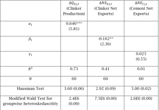
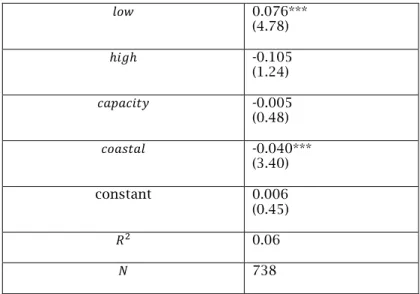
3.4. Estimating counterfactual production and trade
For every installation, we estimate a counterfactual output level, to contrast with the observed one. To do so involves three steps and a number of assumptions (detailed in Appendix C). First, we use a simple fixed effects panel regression to predict clinker production (installation level fixed effects) using regional level cement consumption as the main explanatory variable. Counterfactual cement and clinker export levels are similarly predicted using regional level cement consumption as the main explanatory variable. We find that on average, if cement consumption in a region decreases by 1 Mt, clinker production tends to decrease by 0.65 Mt and clinker net exports increase by 0.16 Mt (see Appendix C.1). This assumes that changes are uniform across all installations in a region. We then relax this assumption and make corrections based on individual plants characteristics calibrated on historic data (see Appendix C.2). In developing the counterfactual, cement consumption and price are assumed to be independent of allocation rules, i.e. they would have been the same in 2012 whatever the allocation scheme considered in the paper. We return to this assumption in Section 3.6."
"""""""""""""""""""""""""""""""""""""""""""""""""""""""""""""
17 The hybrid benchmark avoids the “clinker-cement paradox” (Demailly and Quirion 2006).”. If the benchmarked
product is cement, plants have an incentive to outsource clinker production. If it is clinker, the incentive to reduce the clinker-to-cement ratio is lost. In California, the benchmarked product is “adjusted clinker and mineral additives produced”, which is equal to !!(1 +
!
!), where !!! is the clinker produced, ! is the clinker ratio and ! is the
“mineral additives ratio” (limestone and gypsum consumed divided by cement produced). This system gives an incentive to use more mineral additives while preventing clinker outsourcing.
18 HEL is calculated in the same way as the HAL (Cf. Section 1) but using emissions as a proxy for clinker production
Having estimated counterfactual production levels by installation, we then proceed to estimate the number of free allowances (EUA) received at the plant level under the various
scenarios. As an example, let us consider a plant19, which is functioning at 50% E/HEL and
receiving 1 million EUAs. Suppose that our econometric model finds that the counterfactual activity of this plant is 40%. This plant would have received 0.4 million EUAs under OBA, 1 million EUAs under EX and EXALTG, 0.5 million EUAs under EXALTNG.
In this short example, we see that gaming from 40% to 50% allows obtaining 0.5 MEUAs
more allowances, but involves 0.11 Mt CO2 of additional emissions20, so that the net gain in
terms of allowances is 0.39 MEUAs. To convert the various effects into monetary value, we
assume a CO2 price at 9€/EUA. We consider that the increased production is sold at
marginal cost, and so has no impact on profits.
In summary, for the four different scenarios, we compute production, emissions and allocation. The net allowances (allocation minus emissions) is compared for the scenarios EX, EXALTNG, EXALTG and OBA. Comparing other scenarios to OBA gives an estimation of overallocation profits (in MEAUs or M€). The difference between EXALTG and EXALTNG gives the effect of gaming. Table 1 summarises how allocations and production are obtained under each scenarios.
Table 1: Scenarios
Scenarios Allocations Production
OBA Proportional to Activity (HALxALCF <->q in Eq (1)) Counterfactual (explained in Appendix C) EX Independent of Activity
(ALCF=1 in Eq (1)) Same as OBA
EXALTNG
Hybrid
(Eq (1)) Same as OBA
EXALTG Same as EXALTNG Actual 2012 Production
3.5. Decomposing the destination of excess clinker produced
Which strategies do firms pursue, to increase output and gain free allocations when demand is low? We take a further look at the distortions from ALTs by assessing the relative importance of the different channels through which the excess EU clinker meets its destiny. Comparing counterfactual net exports to real net exports gives the part of the excess clinker production which is destined for clinker exports and cement exports. Assuming no stockpiling, the remaining part is attributed to the change in the clinker ratio.
3.6.. Moderate and low demand countries
We suspect that the most important differences between scenarios EX and EXALTG will occur in countries in which cement and clinker consumption in 2012 fell well short of historical consumption level and hence ALT rules are relevant. The 26 EU ETS member
states21 with ETS-participating clinker production plants, are divided into two groups (see
Table 2). The first group of countries are where the average domestic cement consumption
"""""""""""""""""""""""""""""""""""""""""""""""""""""""""""""
19 Caution, this plant does not have the same characteristics as the one in section 2.2 (in order to make
computations easier)
20 Assuming that the plant has a clinker carbon intensity of 800kg CO
2 per ton of clinker.
21 Note that Iceland, Liechtenstein, Malta have no listed clinker plants in the EUTL database, while data for Cypriote
in 2011-2012 was less than 70% of 2007 levels.22 We name this group “low demand” (LD)
countries. We shall detail some of the results for Greece and Spain, two LD countries particularly affected by the downfall. The LD countries represented 51% of EU ETS cement
emissions in 2008 and 40% in 2012. The remaining countries are classified as “moderate
demand” (MD).
Table 2: Moderate- (MD) and low demand (LD) countries in terms of cement consumption in 2012 relative to 2007 levels23
Low Demand (LD) Countries Moderate Demand (MD) Countries
Ireland, Spain, Greece, Bulgaria, Hungary, Denmark, Portugal, Italy, Slovenia and Baltic countries
Austria, Belgium, Czech Republic, Finland, France, Germany, Netherlands, Norway, Poland, Romania, Slovakia, Sweden and United Kingdom
3.7. Key assumption
In terms of the construction of the counterfactual, our central hypothesis is that cement consumption and price are independent of allocation method. This assumption may at first appear at odds with the economic literature (Fischer and Fox 2007, Demailly and Quirion, 2009). Ex-ante free allocations would ordinarily not provide any protection against leakage (they are a lump sum transfer and firms marginal cost fully support the cost of carbon) while ex-post OBA allocations would (with OBA, firms receive free allocation proportional to their output the marginal cost is unchanged and there are no competitive impacts with respect to imports; this is the usual argument in favour of OBA). Cement consumption and price would then depend on the allocation scheme. This paper departs from this view. Rather, it assumes that firms adopt exactly the same pricing and production decisions in their home market in OBA and ex-ante allocation. This assumption is supported by a series of in depth interviews with cement sector actors (Neuhoff et al, 2014) to explicitly show why there has been no leakage. These interviews point out a number of reasons for such behaviour: The ex-ante free allocations have been obtained precisely to mitigate leakage thus a risk of losing future free allocations if regulators observe the ability to pass on the cost of carbon without observing leakage; the long term risk of attracting new entrants into the market from elevated prices (i.e. limit pricing); the risk of drawing the attention of competition authorities due to abnormal profit levels. This paper finds these arguments persuasive and thus assumes that the allocation rule has no impact on consumption and on prices of cement in the EU. The crux of our analysis concerns their impact on the production of clinker and cement.
3.8. Data
To examine the effects of ALTs on the cement sector, 246 clinker producing installations
were identified as operating in 2010, 2011 and 2012.24 Other variables are obtained at the
country level as summarised in Table 3.
"""""""""""""""""""""""""""""""""""""""""""""""""""""""""""""
22 The average of 2011 and 2012 was taken since both years are relevant to the analysis that follows here. 2007 is
taken as the reference year since this was the year in which demand peaked in most EU Member States prior to the economic crisis of 2008.
23"There are no clinker plants in Malta, Lichtenstein and Iceland. Emissions data on two clinker plants of Cyprus is
available from 2012 only, hence cannot be used in this analysis. "
24 For this purpose, we rely heavily on the work carried out by Branger and Quirion (2014), which has developed an
Table 3: Data sources
Variable Source Emissions and HEL EUTL Clinker net exports
(NEK) Eurostat (http://epp.eurostat.ec.europa.eu/newxtweb/setupdimselection.do# Eurostat (http://epp.eurostat.ec.europa.eu/newxtweb/setupdimselection.do#, International Trade, EU Trade Since 1988 by HS2, 4, 6 and CN8).
Data is originally given by country pairs. Total net exports are re-computed. Product category: “Cement Clinker” (252310)
Cement net exports
(NEC) Eurostat Product category: Difference between “Cement, incl. cement clinkers” (2523) and “Cement Clinker” (252310).
Cement consumption
(CC) 1) Cembureau (2013) for the main European countries
2) VDZ ( http://www.vdz-online.de/en/publications/factsandfigures/cement-sales-and-consumption/, Table C10) for Baltic countries and Norway. Clinker production
(QK) EUTL-derived estimation (through estimated clinker carbon intensity and emissions, see A1). Where there were data gaps, supplementary data were obtained from several sources e.g.:
• National cement association data when reliable and exploitable, i.e. Spain (https://www.oficemen.com/Uploads/docs/Anuario%202012%281%29 .pdf, p90) • Germany ( http://www.vdz-online.de/en/publications/factsandfigures/cement-data-at-a-glance/, table A2) • France ( http://www.infociments.fr/publications/industrie-cimentiere/statistiques/st-g08-2012, Table p7)
• Getting the Numbers Right database (GNR,
http://wbcsdcement.org/GNR-2012/index.htmlhttp://wbcsdcement.org/GNR-2012/index.html, indicator 311a) for available countries (UK, Italy, Poland, Czech Republic, Austria)
4. Results
4.1. Impact of ALTs on the plant distributions
Figure 2 displays the distribution of plant activity levels for 2012 (EXALTG), the counterfactual production (EX, EXALTNG, OBA) and also the distribution in 2011 for comparison. In LD countries, there is a marked jump in installations operating around the 25% and 50% activity level thresholds in 2012, whereas the counterfactual distribution for these countries is not skewed at the thresholds. We find that in LD countries where 117 of the 246 cement installations are located, ALTs should have reduced free allocations in 42 of them, but due to gaming, it was reduced in only 20 installations in reality. Thus, in line with preliminary findings of Neuhoff et al (2014), these results show clearly that cement companies have indeed altered plant production levels in response to ALT rules. In MD countries, this response is noticeable but to a much less degree. The contrast between LD and MD shows the importance of the demand collapse in triggering this gaming behaviour.
Figure 2: Distribution of installations according to their activity level (approximated by E/HEL) in 2012 for observed and counterfactual production.
"
4.2. ALT impacts on clinker production and emissions
Table 4 gives the clinker production and the emissions for 2012 (EXALTG) and the counterfactual (EX, EXALTNG, OBA). The excess clinker production due to the introduction of thresholds rule is quantified. It represents an increase of 12% in LD countries, 21% for Spain and 42% for Greece. These increases are extremely large, even if the global impact at the EU level is more modest (5%). The increase in the clinker production translates into
increases in emissions. Altogether we estimate that an additional 5.2 Mt CO2 (+5 % for the
0" 10" 20" 30" 40" 50" N u m b er 'o f'i n st al la ti on s' 2012'3'LD'Countries' 0" 10" 20" 30" 40" 50" N u m b er 'o f'i n st al la ti on s' 2012'3'MD'Countries' 0" 10" 20" 30" 40" 50" N u m b er 'o f'i n st al la ti on s' 2012CF'3'LD'Countries' 0" 10" 20" 30" 40" 50" N u m b er 'o f'i n st al la ti on s' 2012CF'3'MD'Countries' 0" 10" 20" 30" 40" 50" N u m b er 'o f'i n st al la ti on s' 2011'3'LD'Countries' 0" 10" 20" 30" 40" 50" N u m b er 'o f'i n st al la ti on s' 2011'3'MD'Countries'
sector as a whole) have been emitted by EU cement firms as a consequence of the strategic
behaviour of cement companies25.
Table 4: Production and Emissions for the observed (EXALTG) and counterfactual (EX, OBA, EXALTNG) scenarios
LD
countries MD countries All countries Spain Greece Production (CF) in Mtons 48.7 79.3 127.9 13.2 3.9 Production (observed) in Mtons 54.4 79.4 133.8 16.0 5.6 Increased Production in Mtons 5.7 0.1 5.8 2.7 1.7 Emissions (CF) in Mtons CO2 42.7 67.5 110.2 11.4 3.5 Emissions (observed) in Mtons CO2 47.8 67.6 115.3 13.7 5,0 Increased emissions in Mtons CO2 5.1 0.1 5.2 2.4 1.5
4.3. Impact of gaming on plant distribution on the free allowances
Table 5 gives the amount of EUA’s that are allocated to cement installations under the four scenarios (EX, EXALTNG, EXALTG, OBA). If installations received 100% of their allowances regardless of their activity (i.e. the allocation under the EX scenario), then LD countries and MD countries would have received 74.5 and 70 million EUAs respectively. OBA allocations would lower allocations to 37.1 and 61.5 million EUAs respectively. The decrease in allocations is more significant for LD countries because the average activity is much lower. As explained, the scenario EXALTNG can be seen as an imperfect approximation of the OBA rule. If there had been no gaming, it would have set the allocations at 58.7 and 68.6 million EUAs. Thus for the cement sector as a whole, ALTs reduced overallocation in 2012 by 6.6 MEUSs compared to the scenario without ALTs. Had OBA been implemented instead, overallocation would have been further reduced considerably by 39.5 MEUAs, which corresponds to 29% of the total cement sector free allocation in 2012. The theoretical effect for the MD countries is negligible, as most of installations have an activity level superior to 50%. However for LD countries the theoretical effect of the threshold rule as an approximation of the OBA rule would have been more significant: a 42% (that is (74.5 – 58.7)/(74.5 – 37.1)) reduction should have been obtained. With gaming (EXALTG) a reduction of only 16% prevails (that is (74.5 – 68.4)/(74.5 – 37.1)). For Spain the percentages would respectively be 57% and 21%; and for Greece 71% and 24%.
Table 5: The Free Allowances (MEUAs) under the four scenarios
Allocations LD countries MD countries All countries Spain Greece
EX 74.5 70.0 144.5 23.6 8.7
EXALTNG 58.7 68.6 127.4 15.8 4.6
EXALTG 68.4 69.6 138.1 20.7 7.3
OBA 37.1 61.5 98.6 10.0 2.9
4.4. Financial potential gain associated with gaming
In the calculation of the potential gain we assume that the increased production is sold at marginal cost, and so has no impact on profits. This gives an upper bound for the profits that could be achieved with gaming since it does not take into account the possible inefficiency costs: logistics cost for production shifting, extra sales expenditures and rebates for increased exports, opportunity cost for increasing the clinker to cement ratio).
"""""""""""""""""""""""""""""""""""""""""""""""""""""""""""""
25 This increase can be decomposed as 5.1 Mt CO
2 due to a scale effect (more production) and 0.1 Mt CO2 due to an
That there are inefficiency costs can be seen from the fact that not all plants achieved the 50% threshold, but some gaming was certainly worthwhile since a large proportion of plants did manage to get to the target.
To convert the increase in free allowances and the increase in emission rights into monetary
value, we need to assume a CO2 price. It should be clear that the amount of profitable
gaming is dependent on the CO
2 price. We shall come back to this point in our discussion of
the results.
Table 6 gives the potential profit associated with gaming for a CO2 price at 7.95€/t, which
corresponds to the average future price (December 2013) during year 2012.26
Table 6: Quantification of the monetary value of excess free allocations for the various scenarios.
Millions of €
relative to OBA LD MD All Spain Greece
EX 297 68 365 109 46
EXALTNG 172 57 228 47 14
EXALTG 208 64 272 67 23
For LD countries, the potential gain of EX relative to OBA is estimated through the net
increase of allowances which is 74.5 – 37.1 Mt CO2 and a EUA price 7.95€/t which makes 297
M€. With the introduction of the threshold rule this increase would have been only 172 M€ had the firms not gamed the scheme. The reduction is coming from the reduced amount of free allocations due to the downfall in market demand.
The gaming increases the amount of free allocations but increases emissions, bringing a
potential gain at 208 M€, which represents an increase of 18% relative to 172 M€.27 For Spain
the per cent increase is 41% and for Greece it is 62%. These figures are substantial even though the carbon price was low at that time. This explains why firms indulge in the various inefficiencies described earlier to capture part of this gain.
4.5. Where does the excess clinker end up? Indirect evidence revisited
This section revisits the indirect evidence of excess clinker production proposed by Neuhoff et al. (2014). As noted, three channels have been identified, production shifting, exports increase and clinker ratio increase.
a) Production shifting in multi-plants companies. Cement company executives in interviews reported that subsequent to the introduction of ALTs, it was frequent practice to arrange production levels across plants to ensure being above the threshold at as many
units as possible (Neuhoff et al. (2014). We observe output behaviour consistent with these
statements in several cement companies which have a number of plants producing close to
the thresholds. Table 7 presents four examples28. In each of these firms in 2012, production
(within the same geographical region) simultaneous falls in production in one plant which produced well above the threshold in 2011, and rises to above the threshold in another plant which was previously operating below the threshold.
"""""""""""""""""""""""""""""""""""""""""""""""""""""""""""""
26 Source: ICE database (http://data.theice.com/MyAccount/Login.aspx)
27 Note that our methodology estimates the overallocation profit using the level of free allocations for year 2013
based on activity levels in year 2012 while their emissions in 2013, for which they have to pay certificates, depend on actual emissions in 2013, while we use the counterfactual for 2012.
28 We only display here groups of installations belonging to a country-company that are the most consistent with
production shifting, but avoid cherry-picking individual installations. For the four cases, all installations of a certain country-company are displayed.
Table 7: Evidence of within-firm-country production shifting to meet thresholds
Country-Company Installation E/HEL 2011 E/HEL 2012
Greece-W 1 34% 49% Greece-W 2 77% 66% Greece-W 3 11% 0% Spain-X 1 42% 50% Spain-X 2 57% 46% Spain-X 3 68% 56% Hungary-Y 1 41% 46% Hungary-Y 2 68% 50% Portugal-Z 1 34% 64% Portugal-Z 2 55% 51% Portugal-Z 3 71% 60%
Note: We recall that if E/HEL>45%, then the installation is above the threshold
b) Exports. Table 8 gives net exports of clinker and clinker embedded in cement from 2010 to 2012 for LD and MD countries. We observe a surge in clinker net exports in LD countries: 5.88 Mt in 2012, compared to 1.94 Mt and 1.56 Mt in 2010 and 2011 respectively. In contrast MD countries remained small net importers of clinker and no significant shift was observed in their trade patterns. Further analysis revealed that these clinker exports in 2012 were destined mainly to countries in Latin America and Africa, including Brazil, Togo, Ghana, Cameroon, Côte d’Ivoire, and Mauritania and Nigeria, which could have imported from Non EU various sources.
Table 8: Clinker net exports in 2010, 2011 and 2012 in LD and MD countries in millions of tonnes
LD Countries 2010 2011 2012 Clinker 1.94 1.56 5.88 Clinker in Cement 5.12 4.09 5.75 MD Countries 2010 2011 2012 Clinker -0.87 -0.43 -0.37 Clinker in Cement 2.39 2.78 2.63
Note: Source: Eurostat we use a common clinker ratio of 75% to compute clinker embedded in cement
c) Clinker ratio. Another way excess clinker production might materialise is in a higher clinker-to-cement ratio. That is, firms could use more clinker to produce the same ton of cement. The clinker ratio can be recomputed at the macro level (state of group of states)
with the formula!! =!!!!"!
!!!!"!, where !! is the clinker production, !"! and !"! net exports
of clinker and cement, and !! the cement consumption (see Appendix B for explanation and
Table 3 for data source).
Table 9 shows the clinker ratio for the MD countries, LD countries, Spain and Greece. The historical declining trend in the clinker-to-cement ratio has reversed in 2012.
Table 9: Clinker-to-Cement Ratio in selected areas (source: authors' analysis)
Clinker Ratio 2010 2011 2012
MD Countries 76% 76% 77%
LD Countries 74% 72% 74%
Spain 79% 76% 82%
4.6. Decomposing the channels for clinker disposal
Our econometric model allows for deriving counterfactuals for net exports of clinker and cement (See Appendix C). Assuming no stockpiling, we can attribute the remaining excess clinker output to clinker ratio increase thereby decomposing into three destination channels. The cement consumption was remarkably low in 2012. Because of the consumption/export relationship established by the econometric model, clinker net exports would have risen anyway in 2012 compared to 2011 had the threshold rule not be implemented. This point need be taken into account in the analysis.
Table 10 details the results. Figure 3 provides a graphical representation. For LD countries, net exports of clinker increased by 6.2 Mt while our counterfactual is 4.6 Mt (+1.6 Mt); the net export of cement increased by 8.5 Mt while the counterfactual is 6.1 Mt (+1.7Mt of clinker embedded); this implies that 2.4 Mt of clinker went into the increased content of clinker in cement. This latter figure represents an increase of 4% relative to our counterfactual for the clinker to cement ratio as defined in the previous section.
Table 10: Real and counterfactual net exports of clinker and cement (Mt)
Total
Increase Clinker Net Exports 2012 Cement Net Exports 2012 Clinker Ratio Region Production Clinker CF Obse rved Diff CF Obse rved Diff*R Effect Relative All LD 5.7 4.6 6.2 +1.6 6.1 8.5 +1.7 2.4 + 4% All MD 0.1 0.4 -0.7 -1.1 3.3 2.7 -0.4 1.7 + 2% All 5.8 5.0 5.5 +0.5 9.4 11.2 +1.3 4.0 + 2% Spain 2.7 2.2 3.4 +1.2 2.2 2.6 +0.3 1.2 + 7% Greece 1.7 0.5 1.8 +1.3 1.5 1.7 +0.2 0.2 + 4%
Figure 3: Routes of excess clinker
5. Conclusions and policy options
An important change in the EU-ETS phase 3 for EITE concerns the introduction of the activity level threshold rule (ALT). The underlying rationale for its introduction is that it
(2" 0" 2" 4" 6"
All"LD" All"MD" All" Spain" Greece"
Mt'of'c lin ker'
Routes'of'excess'clinker'production'(Real'vs.'
Counterfact)'Decomposition'
Clinker"Exports"Increase" Cement"Exports"Increase" Clinker"Ratio" Total"Increase"would reduce the overallocation profits in case of downfall in the demand: whenever the activity level of an installation falls below some threshold (50%, 25%, 10%) relative to its historic activity level used to allocate free allocations, the allocation would be reduced accordingly (50%, 25%, 0%).
Our ex post analysis of year 2012, the first year in which the threshold rule applies, focused on the cement sector, a sector in which approximately half the EU countries had experienced a significant downfall in consumption (LD countries). It provides a natural experiment to evaluate the consequences of this rule.
Our main conclusion is that while ALT did reduce to some extent overallocation profits, it also created operational distortions which lead to outcomes inconsistent with the low carbon transition of EU energy intensive industries. The reduction in overallocation profits is less than expected because of the gaming behaviour of the industry to achieve the thresholds, during periods of low market demand. Thanks to the elaboration of a counterfactual, we have been able to quantify that after the introduction of ALTs: the potential overallocation profit with gaming is 272 M€ (2 €/t clinker) and 228 M€ without gaming, while it would have been 365 M€ in the absence of ALT. The expected reduction in windfall profits due to the ALT is 38% while the actual reduction is 25%. The incentives are magnified in low demand countries, where profit with gaming is 208 M€ (3.8 €/t clinker) and 172 M€ without gaming, while it would have been 297 M€ without ALTs. We examined three ways in which firms’ operations are altered in response to ALTs: shifting production among plants, increasing net exports of clinker and cement, increasing the clinker to cement ratio. In the 2000’s top management attention on the issues of climate change emerged as an important dimension of corporate social responsibility and a large number of companies got involved into proactive strategies to limit their own emissions (Arjalies et al., 2011). The EU-ETS positively contributed to turn this strategy into operational practise by putting a price on carbon. The distortions reported in our study are particularly detrimental in this respect: the production shifting goes against the restructuring of the assets to achieve scale economies, a key factor of cost efficiency in cement; the increased exports induce some relocation of foreign cement consumption in the EU, while the EU-ETS intention in giving free allocations was designed to reduce leakage, i.e. the relocation of EU consumption in foreign countries; the increase in the clinker to cement ratio goes against one of the main drivers to limit emissions in cement production. The introduction of ALT reversed the alignment of objectives between corporate social responsibility and the EU-ETS.
Our results have been obtained in a context of low carbon price, severe downfall in market demand, and large free allowances. A higher carbon price would make our results even more
relevant, the higher the carbon price the higher the incentive to achieve the thresholds.29
Had we observed growth, the threshold rule would have been inactive and the reserve for
new entrants rule would have been the issue to be analysed. Anecdotic evidence30 suggests
likely distortions in that case as well and it would be interesting to carry out a rigorous analysis similar to this one.
"""""""""""""""""""""""""""""""""""""""""""""""""""""""""""""
29 Take a EUA price at 20€/t a simple extrapolation for LD countries would bring up the potential wind fall profit to
236*20/9 = 524 M€. However if we assume that all plants achieve the 50% threshold, a reasonable assumption for a EUA price at 20€/t, it would go up to 583 M€. The expected reduction remains at 42% but the actual one drops to 22%.
30 If the historic activity level (HAL) refers to say a 60% capacity utilization rate, increasing production to 80% may
not be beneficial since it will increase emissions with no increase in free allowances; in case of capacity expansion the detailed rule to determine the level of free allowances may induce an artificially high production during the period used to fix that level. Ref. private conversation with industry representatives.
These considerations suggest that the threshold rule should be abandoned for sectors such as cement for which carbon costs represent a significant share of production costs. This raises the question of what to put in its place for such sectors. Theory suggests that replacing free allocation with full auctioning and using border carbon adjustments offers the most efficient solution, yet politically this solution has not yet gained serious traction. Since the problem arises in part because the thresholds create an allocation system that fall between an ex-ante and ex-post scheme, one solution would be to move to full ex-post output-based allocation.
However, a number of issues must be carefully investigated before going in that direction. We can think of the following points: OBA implies the loss of an absolute cap for free allocations, OBA stifles any possibility for prices to be passed down the value chain, OBA may create a heavy administrative burden, and the declining trend in the caps to decarbonize the economy over the long term is incompatible with a benchmark to mitigate leakage. There are on-going discussions on how to circumvent these issues. For example the loss of demand side substitution incentives could be restored with a consumption charge (Neuhoff et al 2014). Output based scheme with hybrid benchmark has been implemented in California in 2012. An ex post study on this implementation would be welcome to see if, again, the devil lies in the details.
Acknowledgements
The authors wish to acknowledge the following people for their helpful comments and suggestions in the writing of this paper: Philippe Quirion, Andrei Marcu, Karsten Neuhoff, Bruno Vanderborght, Luca Taschini, DG Clima and the maintainers of the EUTL public registry, WBCSD and all the people who contribute to the Getting the numbers right (GNR) cement sector database and numerous people from the cement industry. Jean-Pierre Ponssard gratefully acknowledges the financial support from the ANR/Investissements
d'avenir (ANR -11- IDEX-0003-02). Misato Sato gratefully acknowledges financial support
from the Grantham Foundation and the ESRC through the Centre for Climate Change Economics and Policy.
References
Arjalies, D-L., Goubet, C. and Ponssard, J-P. (2011) Approches stratégiques des émissions CO
2 Les cas de l’industrie cimentière et de l’industrie chimique. Revue Française de Gestion,
215, 123-146 (english version available at
http://papers.ssrn.com/sol3/papers.cfm?abstract_id=2287784 )
Boyer, M. and Ponssard, J.-P. (2013), Economic Analysis of the European Cement Industry. CIRANO - Scientific Publication No. 2013s-47. http://dx.doi.org/10.2139/ssrn.2370476 Branger, F and Quirion, P (forthcoming) Reaping the carbon rent: abatement and over-allocation profits in the European cement industry, insights from a LMDI decomposition analysis.
Branger, Frédéric, Philippe Quirion, and Julien Chevallier. Carbon Leakage and
Competitiveness of Cement and Steel Industries under the EU ETS: Much Ado about Nothing. Working Paper CIRED, 2013.
California Air Resources Board (2013) California Cap on Greenhouse Gas. Emissions and
Market-Based Compliance Mechanisms.
www.arb.ca.gov/cc/capandtrade/c-t-reg-reader-2013.pdf
CEMBUREAU (2013) World Statistical Review 2001 – 2011, available from < http://www.cembureau.eu/world-statistical-review-2001-2011>
Demailly, D., Quirion, P. (2006) CO2 abatement, competitiveness and leakage in the European cement industry under the EU ETS: grandfathering versus output-based allocation. Climate Policy 6:93–113
Demailly, D. and Quirion, P. (2008). Leakage from climate policies and border tax
adjustment: lessons from a geographic model of the cement industry, in: R. Guesnerie, H. Tulkens (eds), The Design of Climate Policy, The MIT Press, Boston, MA, 333_358.
Ellerman, A. Denny, Paul L. Joskow, Richard Schmalensee, Juan-Pablo Montero, and Elizabeth M. Bailey. 2000. Markets for Clean Air: The U.S. Acid Rain Program. Cambridge, United Kingdom: Cambridge University Press.
Ellerman, A. D. (2008). New entrant and closure provisions: how do they distort? The Energy Journal, (pp. 63–76).
Ellerman, A., Convery, F., De Perthuis, C. and Alberola, E. (2010). Pricing carbon: the European Union emissions trading scheme, Cambridge University Pr.
EUTL. European Union Transaction Log, European Commission,
http://ec.europa.eu/environment/ets/ (accessed February 2014)
European Commission (2011). Decision 2011/278/EU on determining Union-wide rules for harmonised free emission allowances pursuant to Article 10a of Directive 2003/87/EC, European Commission, Brussels.
European Commission (2009) Attribution of list of NACE codes to CITL installations, published on the DG Competition website, European Commission, Brussels, (accessed September 2013)
http://ec.europa.eu/dgs/competition/index_en.htmhttp://ec.europa.eu/dgs/competition/in dex_en.htm
European Commission (“EC”). (2003). Determining, pursuant to Directive 2003/87/EC of the European Parliament and of the Council, a list of sectors and subsectors which are deemed to be exposed to a significant risk of carbon leakage (2010/2/EU).
European Climate Foundation, ECF (2014) Europe’s low-carbon transition: understanding the challenges and opportunities for the chemicals sector, European Climate Foundation,
Brussels.
Fischer, C. and Fox, A. K. (2007). Output-based allocation of emissions permits for mitigating tax and trade interactions. Land Economics, 83(4): 575-599.
Fischer, C. and Alan K. Fox, 2012, Comparing policies to combat emissions leakage: Border carbon adjustments versus rebates, Journal of Environmental Economics and Management, 64(2): 199 216.
Fowlie, M., Reguant, M., Ryan, S.P., (2012), Market-based emissions regulation and industry
dynamics., National Bureau of Economic Research, www.nber.org/papers/w18645
Hourcade, J.-C., Demailly, D., Neuhoff_, K. and Sato, M. (2008). Differentiation and dynamics of EU ETS competitiveness impacts: final report. Report, Climate Strategies, Cambridge, section 3: 60_93.
Jensen, M. C. (2001), Paying People to Lie: The Truth About the Budgeting Process (Revised September, 2001). Harvard NOM Research Paper No. 03, and HBS Working Paper No.
01-072. http://dx.doi.org/10.2139/ssrn.267651
Laing, T., Sato, M., Grubb, M. and Comberti, C. (2014). The effects and side-effects of the EU emissions trading scheme. WIREs Clim Change, DOI:10.1002/wc.283
Locke, E. A. (2001). Motivation by goal setting. In Golembiewski, R. T. (ed.), Handbook of Organizational Behavior. New York: Marcel Dekker.
McKinsey&Company (2008), Pathways to a Low Carbon Economy: Version 2 of the Global Greenhouse Gas Abatement Curve
Meunier, G., Ponssard, J-P. and Quirion, Ph. (2014) Carbon leakage and capacity-based allocations: Is the EU right? Journal of Environmental Economics and Management Volume 68, Issue 2, September, 262–279.
Meunier, G. and Ponssard, J-P. (2014) Capacity decisions with demand fluctuations and carbon leakage. Resource and Energy Economics 36, 436-454.
Neuhoff, K, B. Vanderborght, A. Ancygier, A.T. Atasoy, M. Haussner, R. Ismer, B. Mack, R. Martin, N. Sabio, J.P.Ponssard, P. Quirion, A. van Rooij, O. Sartor, M. Sato (2014) Carbon control and competitiveness post 2020: The cement report, Climate Strategies, 2014, London. February 2014.
Neuhoff,K.,Martinez,K.K.,& Sato,M.(2006). Allocation,incentivesanddistortions: the impact of EU ETS emissions allowance allocations to the electricity sector. Climate Policy, 6(1), 73–91. Oficemen (2013) Anuario del sector cementero español 2012, Oficemen, Agrupacion de fabricantes de cemento de Espana.
https://www.oficemen.com/Uploads/docs/Anuario%202012%281%29.pdfhttps://www.ofice
men.com/Uploads/docs/Anuario%202012%281%29.pdf
Pahle, M., Fan, L., & Schill, W.-P. (2011). How emission certificate allocations distort fossil investments: The German example. Energy Policy, 39(4), 1975–1987.
Quirion, P., 2009. Historic versus output-based allocation of GHG tradable allowances: a survey. Climate Policy, 9: 575-592.
Sallee, J. M. & Slemrod, J. (2012). Car notches: Strategic automaker responses to fuel economy policy. Journal of Public Economics, 96(11–12), 981–999.
Sandbag (2011). Carbon Fat Cats 2011: The Companies profiting from the EU Emissions Trading Scheme. Report, Sandbag Climate Campaign. Available from:
http://www.sandbag.org.uk/site_media/ pdfs/reports/Sandbag_2011- 06_fatcats.pdf.
Sartor, O., Pallière, C., Lecourt, S. (2014): Benchmark-based allocations in EU ETS Phase 3: an
early assessment, Climate Policy, published online. DOI: 10.1080/14693062.2014.872888
WBCSD (2014) Getting the Numbers Right database, Cement Sustainability Initiative,
accessed February 10, 2014,
http://www.wbcsdcement.org/index.php/key-issues/climate-
protection/gnr-databasehttp://www.wbcsdcement.org/index.php/key-issues/climate-protection/gnr-database
WBCSD (2011), CO
2 Energy Accounting and Reporting Standard for the Cement Industry
2011: The Cement CO2 Protocol, Cement Sustainability Initiative, WBCSD, Geneva.
Appendix
A. EUTL Data computations'
A.1 Determination of the Activity Level Correction Factor (ALCF2013) at the plant level
The key challenge is to correctly distinguish installations that are above or below thresholds (25% and 50% of q/HAL), despite the limitation that activity levels have to be approximated using emissions data (E/HEL). To do so, we exploit the observations from the 2013
allocation data, which revealed whether or not the installation had seen its allocation reduced because its 2012 activity level fell below a threshold. Allocations in 2013 are equal to (cf equation (1)):
!!,!"#$= !"!#!"!"×!!×!"#!×!"#$!,!"#$
Where !"!#!"#$ is the 2013 Cross Sectoral Correction Factor (0.9427), !! the clinker carbon
intensity benchmark (766 kg CO
2 per ton of clinker), and !"#! the Historical Activity Level
of installation ! (in tons of clinker). Transforming the previous equation, where both !"#!
and !"#$!,!"#$ are unknown, we obtain:
!"!#!"#$× !!! !×!"#! !!,!"#$ = 1 !"#$!,!"#$× !!,!"# !! Noting !!,!"#=!"#!"#!
! (corresponding approximately to the clinker carbon intensity for the HAL
producing years), and !! is the average clinker carbon intensity (863 kg CO2 per ton of
clinker, GNR, indicator 321) in 2008. We chose 2008 to proxy HAL production (not the highest level of production, which is 2007, but close).
The ratio at the left part of the equation can be computed with available data. On the right part, we have !"#$!,!"#$, which we want to find, and the ratio,!
!!,!"#
!! , which is unknown as
well but bounded and likely to be close to 1. Indeed, !!,!"# varies in an extreme range from
720 kg CO2 per ton of clinker to 1300 kg CO2 per ton of clinker (and for the very large
majority of the plants from 780 to 950 kg CO2 per ton of clinker), which translates into a
ratio !!,!"#
!! varying from 0.83 to 1.51 (and most likely from 0.90 to 1.10). Then, if the ratio, is
comprised between 0.83 to 1.51 (respectively between 1.67 and 3.01, and between 2.64 and 4.8031), we infer that !"#$
!,!"#$ = 1, (respectively 0.5 and 0.25).
This enabled catching out situations in which imperfections in the E/HEL measure as a proxy for the q/HAL would have led to a false conclusion about whether an installation was truly above or below its activity threshold in 2012. We found that the actual thresholds for the E/HEL measure that matched the 2013 allocation data were slightly lower in practice, at 22% and at 45%, rather than 25% and 50%. Discussion with industry experts revealed that there was a logical explanation for this systematic bias: clinker producers often have more than one kiln inside an installation that is treated as a single unit for free allocation purposes. When demand falls, it is common to concentrate production in the most efficient kiln(s). Thus emissions may fall by slightly more than overall clinker production, creating a slight downward bias in E/HEL as a measure of q/HAL in low demand countries. This bias could also be explained by the clinker carbon intensity improvement between HAL years and 2012.
A.2 Determination of clinker carbon intensity at the plant level
Once the !"#$!,!"#$ has been determined at the plant level ! (see previous section), the plant
clinker carbon intensity for HAL years, !!,!"#, can then be obtained with the previous
equation.
For 20 plants (out of 246), we found an unusual number (below 700 kg CO
2 per ton of
clinker), possibly due to a capacity increase, and put instead a default value equal to !!.We