AVC to HEVC transcoder based on quadtree limitation

HAL Id: hal-01433749

https://hal.archives-ouvertes.fr/hal-01433749

Submitted on 28 Feb 2020

HAL is a multi-disciplinary open access

archive for the deposit and dissemination of

sci-entific research documents, whether they are

pub-lished or not. The documents may come from

teaching and research institutions in France or

abroad, or from public or private research centers.

L’archive ouverte pluridisciplinaire HAL, est

destinée au dépôt et à la diffusion de documents

scientifiques de niveau recherche, publiés ou non,

émanant des établissements d’enseignement et de

recherche français ou étrangers, des laboratoires

publics ou privés.

Elie Gabriel Mora, Marco Cagnazzo, Frederic Dufaux

To cite this version:

Elie Gabriel Mora, Marco Cagnazzo, Frederic Dufaux. AVC to HEVC transcoder based on quadtree

limitation.

Multimedia Tools and Applications, Springer Verlag, 2017, 76 (6), pp.8991-9015.

�10.1007/s11042-016-3498-8�. �hal-01433749�

AVC to HEVC transcoder based on quadtree

limitation

Elie Gabriel Mora, Marco Cagnazzo, Senior Member, IEEE, and Frederic Dufaux, Fellow, IEEE

Abstract—Following the finalization of the state-of-the-art High Efficiency Video Coding (HEVC) standard in January 2013, sev-eral new services are being deployed in order to take advantage of the superior coding efficiency (estimated at 50% less bitrate for the same visual quality) that this standard provides over its predecessor: H.264 / Advanced Video Coding (AVC). However, the switch from AVC to HEVC is not trivial as most video content is still encoded in AVC. Consequently, there is a growing need for fast AVC to HEVC transcoders in the market today. While a trivial transcoder can be made by simply cascading an AVC decoder and an HEVC encoder, fast transcoding cannot be achieved. In this paper, we present an AVC to HEVC transcoder where decoded AVC blocks are first fused according to their motion similarity. The resulting fusion map is then used to limit the quadtree of HEVC coded frames. AVC motion vectors are also used to determine a better starting point for integer motion estimation. Experimental results show that significant transcoder execution time savings of 63% can be obtained with only a 1.4% bitrate increase compared to the trivial transcoder.

Index Terms—HEVC, AVC, transcoding, quadtree limitation.

I. INTRODUCTION

T

HE state-of-the-art High Efficiency Video Coding stan-dard [1], developed by the Joint Collaborative Team on Video Coding (JCT-VC) of ISO and ITU, reached Final Draft International Status (FDIS) in January 2013. HEVC allows up to 50% bit-rate reduction at the same visual quality compared to its predecessor, the H.264 / Advanced Video Coding (AVC) standard [2]. These gains reduce the bandwidth load of content providers and enable Ultra High Definition (UHD) applications which were difficult to deploy with pre-vious codec generations due to the large bit-rates required to code such high resolution videos. Today, while dedicated HEVC encoder systems are not yet deployed on a large scale, HEVC software decoders have already started to surface. HEVC codecs are even being included in the latest generation of smartphones [3]. However, most of the video content is still encoded in AVC, due to the wide adoption of AVC in broadcast over cable and satellite, conversational applications over wireless and mobile networks, and multimedia streaming services. Consequently, there is a need in the market for a fast, possibly real-time, AVC to HEVC transcoder to enable interoperability between AVC streams and HEVC services when they will be deployed, or simply to take advantage of the improved coding efficiency that HEVC provides. Indeed, our preliminary experiments show that in a random access E.G. Mora is with ATEME, France; M. Cagnazzo and F. Dufaux are with LTCI, CNRS, Tlcom ParisTech, Universit Paris-Saclay, 75013, Paris, France (e-mail:

{elie-gabriel.mora,marco.cagnazzo,frederic.dufaux}@telecom-paristech.fr)

configuration, transcoding AVC streams into HEVC brings up to 20.7% bit-rate reduction compared to AVC.

Video transcoders serve many purposes [4]–[6]. They come in two types: homogeneous and heterogeneous transcoders. Homogeneous transcoders keep the video content in the same format used in the initial encoding stage. They are used for instance to reduce bit-rate or to adjust spatial or temporal resolutions [4]. Another application consists in adapting the coding rate to the user requirement or to the constraints of the network or of the storage devices. Other applications of homogeneous transcoders include rate control (VBR to CBR and vice versa) and adding scalability layers . as suggested for example in [7] in order to address video distribution on mobile devices. From this point of view, transcoding is seen as a preeminent part of any multimedia distribution system aiming to provide universal access. Heterogeneous transcoders are mostly used to perform a change between different coding standards [4], [8]. As for the transcoder architecture, the literature typically distinguishes open-loop versus closed loop architectures and spatial (or pixel) domain versus frequency domain architectures. This classification is very well described [4], [6] to which, for the sake of conciseness, we refer the interested reader.

In the case of heterogeneous transcoding, such as the AVC-to-HEVC case considered in this paper, a trivial transcoder can be formed by simply cascading an AVC decoder and an HEVC encoder. This approach, called “Full Decode Full Encode” (FD-FE), achieves the best coding performance but it is also the most complex and time consuming. Basically, the target of transcoding is to achieve a significant execution time reduction with the least bit-rate increase. In order to do so, decoded information from the input AVC stream must be exploited to reduce the number of operations performed by the HEVC encoder. Indeed, HEVC uses a quadtree coding structure [9] and in the current reference software HM-13.0 [10], a complex Rate Distortion Optimization (RDO) process is used at each depth level of the quadtree to evaluate the Lagrangian (or RD) cost of each coding mode / partition size combination and to select afterward the configuration yielding the lowest coding cost. Several tests are thus performed. The most time consuming tests are Inter mode tests where motion estimation is performed. In HM-13.0, a motion search area is defined where several positions at integer, half and quarter pixel accuracy are tested.

The AVC to HEVC transcoding schemes found in literature can be classified into either mode mapping schemes or motion vector reuse schemes. In the mode mapping category, AVC information is used by the HEVC encoder to decide to either

skip some coding modes / partition size tests, or to stop the quadtree splitting operation [11]–[15]. In the motion vector reuse schemes, the motion estimation process within Inter tests is simplified by skipping some positions to test using decoded AVC motion information [16]–[20]. A detailed analysis of the state of the art for AVC-to-HEVC transcoder is provided later on in this paper (Section II-C).

Although AVC macroblocks have a fixed size of 16×16, we find that adjacent AVC blocks sharing the same motion information can be fused into a larger block at a lower depth level. By recursively fusing AVC blocks up to the corresponding maximum block size in HEVC, the fused AVC coding structure becomes similar to an HEVC quadtree, and can thus be used to limit it. In this paper, we propose a fusion algorithm and a quadtree limitation method (inspired by a similar work of ours in the context of 3D-HEVC [21]) coupled with a motion vector reuse scheme where AVC motion vectors are used to determine a better starting point for integer motion estimation. The proposed solution achieves 63% transcoder execution time savings while only increasing the bit-rate by 1.4% on average compared to the trivial transcoder in a random access configuration.

While it is true that some state-of-the-art transcoders al-ready employ block fusion, the particular way the fusion is performed here and the criterion on which the fusion is based are original. Furthermore, the quadtree limitation scheme is different from the scheme proposed in [21], and is particularly adapted to the AVC-to-HEVC transcoding problem where it serves as an original mode mapping technique. Finally, while the motion vector reuse scheme used in this paper has been used in prior state-of-the-art work, we find that it completes rather intuitively the proposed solution while providing additional gains that are interesting to report. This makes the proposed method substantially novel; it cannot simply be deduced from previous works.

In summary, the main contributions of this work are the following:

1) a fusion algorithm (FA) allowing to obtain, from the H.264/AVC stream, a quadtree that will be used to guide the HEVC encoder;

2) a quadtree limitation algorithm (QTL) that reduces the number of partitions to be tested by the HEVC encoder — FA and QTL are intended to reproduce the same coding structure as (or a coding structure very close to) a FD-FE transcoder but with reduced computation; 3) the combination of FA+QTL with two existing motion

vector reuse strategies (MVR and MVR2) that further improve the trade-off between execution time and com-pression performance of the transcoder;

4) and finally, an extensive experimental validation of the proposed transcoder on the full HEVC sequence test set, and a comparison with available state-of-the-art transcoders.

The remainder of this paper is organized as follows: Sec-tion II gives an overview of the AVC and HEVC coding structures, of the motion estimation process in HM-13.0, and of the AVC to HEVC transcoders found in literature. Section III presents the proposed method. Experimental results

are reported in Section IV and compared to those of the state of the art. Finally, Section V concludes this paper while highlighting possibilities for future work.

II. BACKGROUND A. AVC and HEVC coding structures

In AVC, slices are divided into macroblocks (MB) of fixed size 16×16 [2]. Each MB is associated with a coding mode. There are three main coding modes in AVC: Inter, Intra and Skip / Direct. The Skip / Direct mode can be considered as a particular Inter mode where the motion parameters (motion vectors and reference indexes) of the MB are derived from decoded information (no motion estimation is performed). A MB coded in a particular mode can be partitioned in the following way:

• Skip / direct: 16×16 • Intra: 16×16, 8×8, 4×4

• Inter: 16×16, 16×8, 8×16, 8×8

In Inter mode, if the MB is partitioned into four 8×8 blocks, each 8×8 block can be further partitioned into either two 8×4, 4×8 or four 4×4 sub-blocks. It is important to note that each partition has its own prediction information (motion parameters in Inter or Skip / Direct modes, Intra directions in Intra mode).

In HEVC [1], a slice is divided into coding tree units (CTUs). Each CTU can then be split into four coding units (CU), and each CU can be further split into four CUs, and so on. A maximum CU size and a maximum depth level are set to limit the CU split recursion. This quadtree approach allows having different block sizes inside the same image, making the encoding more adapted to the image content. Note that a specific coding mode (Intra, Inter, or Merge) is chosen at the CU level. Note also that the Merge mode is a particular Inter mode in HEVC where motion parameters are derived from neighboring blocks. A CU can further be partitioned into prediction units (PUs) where all PUs are coded in the same coding mode, but each PU has its own prediction information. The PUs however cannot be further partitioned. Different coding modes imply different possible PU partitions:

• Merge: 2N×2N

• Intra: 2N×2N, N×N (only possible at the maximum

depth level)

• Inter: 2N×2N, 2N×N, N×2N, 2N×nU, 2N×nD,

nL×2N, nR×2N and N×N (only possible at the max-imum depth level)

In HM, the RDO process computes an RD cost J (J =

D + λR, where R is the rate, D the distortion, and λ a weight

factor) for each coding mode / partition size combination. The cost of splitting the CU is also computed and the configuration yielding the lowest cost is selected. In HM-13.0, the maximum and minimum CU sizes are respectively 64×64 and 8×8, and Inter N×N is disabled. Fig. 1 illustrates all the possible coding modes and partition sizes in AVC and HEVC.

B. Motion estimation in HM-13.0

In HM-13.0, an integer motion estimation (ME) is per-formed, followed by a half-pel and a quarter-pel ME.

Intra_16x16 Intra_8x8 Intra_4x4

Inter_16x16 Inter_8x16 Inter_16x8 Inter_8x8

8x8 4x8 8x4 4x4 P_SKIP B_DIRECT

Intra_2Nx2N Intra_NxN Merge_2Nx2N

Inter_2Nx2N Inter_Nx2N Inter_2NxN Inter_NxN

Inter_2NxnU Inter_2NxnD Inter_nLx2N Inter_nRx2N

Asymetric Motion Partitions (AMP)

AVC HEVC

Fig. 1. Coding modes and partition sizes in AVC and HEVC

1) Integer ME: When estimating a motion vector (MV) for

a PU, a motion vector predictor (MVP) is first derived from neighboring PUs [22]. A search window is defined, centered around the pixel p pointed to by the MVP. Instead of per-forming a time-consuming full search wherein all the positions inside the search window are tested by RDO (by computing an RD cost J ), a more intelligent search pattern, called TZ search [23], is used to reduce the number of tested positions while minimizing coding losses. However we observe that this motion estimation strategy, even though very efficient, is by no mean mandatory. In HM-13.0, a diamond search is performed, during which different diamonds, centered around

p, and of different sizes, are considered. A diamond of size

1 is first processed, then at each iteration, the size doubles and the corresponding diamond is processed until reaching the maximal size which corresponds to the search window. For each diamond pattern, only a small number of points on the diamond perimeter are tested by RDO. In the end, the point with the least RD cost is selected as the best point. If the best point is different than p, another diamond search is performed, this time centered around the best point. The same process is repeated recursively until the best point resulting from the diamond search corresponds to the center itself.

Figure 2 illustrates this process. In this example, the search window equals 6. Three diamond sizes are thus considered in each search: 1, 2 and 4 (the next diamond is of size 8 which exceeds the search window). The red point corresponds to the MVP (p). After a first diamond search, the green point is found to be the best point, and hence another diamond search is performed, centered around the latter. After the second search, the blue point is found to be the best point, and similarly, a third diamond search centered around the blue point is performed. In this example, after the third diamond search, the best point is still found to be the blue point. Hence, the search stops.

2) Sub-pixel ME: The 8 half-pel positions directly

sur-rounding the best integer position are tested by RDO. The one minimizing an RD cost is selected as the best point. Then, the 8 quarter-pel positions directly surrounding the half-pel

MVP Search window

Fig. 2. Diamond search in integer motion estimation in HM-13.0 (red: iteration 1, green: iteration 2, blue: iteration 3)

best point are tested by RDO. The best quarter-pel position is finally set as the MV of the tested PU.

C. AVC to HEVC transcoders in literature

AVC to HEVC transcoders in literature employ mode map-ping and motion vector reuse techniques to reduce the HEVC encoding complexity. A mode-mapping transcoder is proposed in [11], where CUs are classified into either background, foreground or hybrid CUs by comparison with a background frame generated using previously decoded frames. Based on the CU classification, either the CU split is stopped or certain modes / partition sizes are not tested. The HEVC decoder is also modified since the method proposes to insert the generated background frame in the list of temporal references of the frames to encode / decode. The transcoder brings -45.6% Bjontegaard Delta Rate (BD-Rate) gain and achieves 53% execution time savings on average compared to the trivial transcoder. The gains come from a normative change which,

in general, is not desired, and the execution time savings may only hold for surveillance video content for which this transcoder is aimed.

Most transcoders employ both mode mapping and motion vector reuse schemes. In [16], a fast AVC to HEVC transcoder is proposed for multi-core processors implementing Wavefront Parallel Processing (WPP) and Single Instruction Multiple Data (SIMD) acceleration. Two conditions are set to limit the CU split recursion for 32×32 CUs and smaller CUs. Furthermore, for 32×32 CUs, some Inter and Intra partition sizes are not tested depending on the number and configuration of 16×16 MBs covered by the CU. For smaller CUs, only the coding mode and partition size of the corresponding AVC block are tested. The mode-mapping and motion vector reuse parts of this transcoder bring 77% execution time savings but the coding losses are not reported.

Zhang et al. [17] propose a Power Spectrum RDO (PS-RDO) model to determine the quadtree and the best motion vector of each PU in Inter frames. In Intra frames, only the quadtree is determined. In an all-Intra and a low delay configurations, the proposed method brings around 70% and 60% encoder execution time savings respectively. However, the coding losses are not provided. Also, the method was implemented in HM-4.0 which, today, is a relatively old HM software version.

Peixoto and Izquierdo, in [18], propose two transcoders. A simple transcoder, Motion Vector Reuse Transcoder (MVRT), based on motion vector reuse is first introduced, where the Intra mode is tested for a CU only if any part of the CU in AVC is coded in Intra, and where only the vectors of AVC blocks covered by an Inter-coded PU are tested at integer pixel level (the default HEVC search is applied at half and quarter pixel accuracy). Another transcoder, Motion Vector Variance Distance (MVVD), is proposed where a similarity metric is computed for each possible CU. It represents the variance of the motion vectors of the AVC blocks covered by the CU. All possible coding mode / partition size combinations are divided into four groups, and based on the similarity metric, for each CU, only certain groups are tested and the CU splitting can be stopped. Also, only the MVs of the AVC blocks covered by a PU are tested at integer pixel level. The two transcoders are evaluated in a low delay configuration with four temporal reference frames. The first scheme achieves 32% execution time savings with 3.6% coding loss, while the second one achieves 54% execution time savings with 6.3% coding loss.

A transcoder based on region feature analysis (RFA) is proposed in [19], where CTUs are classified as low, high or medium complexity CTUs based on the number of bits used to code the corresponding MBs in AVC. Then, the depth range of a CTU is limited based on its class. Furthermore, the AVC MVs covered by a CU are clustered into two regions and based on the clustering shape, certain partition sizes are no longer tested. Also, new MVP candidates are set for each cluster region and the MV search range is limited. This results in 48% execution time savings with 1.7% coding loss in a low delay configuration with four reference frames.

Peixoto et al. propose, in [20], a transcoder referred to as Linear Discriminant Functions (LDF) and which is based on

content modeling. It involves a training stage during which the frames are fully encoded in HEVC. For each of the CUs coded in these training frames, a set of features is stored as well as the decision to split the CU or not chosen by RDO. In the transcoding stage, the class of a CU is determined by comparing its set of features to the saved ones in the training stage and based on the class, the CU split recursion can be stopped. This results in 63% execution time savings with a 3.6% coding loss in a random access configuration, and 65% and 4.1% respectively in a low delay configuration with four reference frames.

In [24], Diaz-Honrubia et al.proposed a multiple frame transcoder that for the motion estimation process, only consid-ers the frames used in H.264/AVC as reference for temporal predictions. In [25], and in a more complete fashion in [15], it is presented a transcoder based on adaptive fast quadtree level decision (AFQLD). The basic idea is to determine the CU depth using a Bayesian probabilistic model. The threshold for decision is computed on line and both information from HEVC and H.264 stream are used in the Bayesian model. The core of the algorithm consists in a data-driven classifier that decider whether splitting or not the current HEVC CU based on a suitable set of features, among which the QP, the characteristics of the residual, the cost function values of the coding modes, see [15] for more details.

Chen et al. propose in [13] a fast mode decision combined with a fast motion estimation algorithm for transcoding (FMD-FME). As for the motion estimation, the H.264 motion vector that is closest to the PU centroid is used for HEVC. If several H.264 are available for the same PU, the median of them is used. The mode decision algorithm is more complicated and depends on the partition of H.264 macroblocks (see [13] for more details). Finally, in [14] FMD-FME is enhanced by considering PU-level information. The proposed transcoding scheme is still complicated but the transcoding performance in terms of BD-Rate increase and transcoding speedup are very close to [13].

While some of these state-of-the-art transcoders can be efficient, the fact remains that the AVC coding structure is never directly used to control the HEVC quadtree in order to reduce transcoding execution time. Indeed, most schemes only influence the HEVC quadtree by avoiding some partition tests or CU splits, but the rationale behind these mode mappings schemes is not based on the AVC coding structure itself. This is understandable because AVC uses MBs of fixed size 16×16 while HEVC CUs can range for instance from 64×64 to 8×8. Therefore the AVC and HEVC coding structures cannot be directly compared as the AVC one (like the one shown in Figure 3(a)) is in general always more partitioned than the HEVC one (Figure 3(b)). Our method translates the MB-based AVC coding structure into a quadtree comparable to that of HEVC. This is done by merging AVC blocks with similar motion together to obtain larger blocks that can be seen as AVC “CU”s and “PU”s. The fused quadtree can then be used to limit the HEVC quadtree and reduce execution time. This mode mapping scheme can also be coupled with a motion vector reuse scheme to obtain additional execution time savings.

(a) AVC (b) HEVC (c) Proposed fused AVC Fig. 3. AVC, HEVC, and proposed fused AVC quadtrees of a frame in the BQSquare sequence

III. PROPOSED METHOD

Our proposed method consists in an AVC fusion algorithm (FA) followed by an HEVC quadtree limitation algorithm (QTL), combined with a motion vector reuse scheme (MVR). We first perform an AVC decoding, which has a relatively low complexity. Then, let us assume that the HEVC encoder is encoding a frame F . The FA provides a quadtree that is used to limit the complexity of the HEVC encoder.

A. Fusion algorithm

The AVC coding structure of F is fused in order to get a fusion map. F is processed CTU by CTU. The fusion within different CTUs can be done in parallel as the fusion of one CTU is completely independent from the fusion of another CTU.

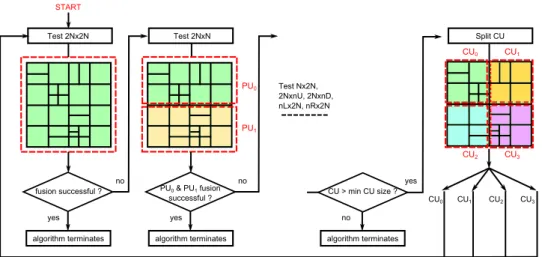
The fusion of a CTU consists in specifying a maximum depth level for CUs and a specific partition for each CU within the CTU. This can be seen as a “fusion” of deeper level CUs, hence its name. The fusion is performed by low complexity processing of AVC decoded information (namely, MVs) and is recursive with respect to the HEVC quadtree structure. More precisely, the fusion of a CTU is described as follows: first, the fusion using a 2N×2N partition is tested. If the fusion is successful (i.e. maximum depth level equals 0), the algorithm terminates and the next CTU is processed. Otherwise, the 2N×N partition is tested. In this case, for the fusion at the CTU level to be successful, the fusion in each of the two PUs must be successful and if so, the algorithm terminates. Otherwise, the N×2N partition is tested, followed by the AMPs: 2N×nU, 2N×nD, nL×2N and nR×2N. If none of the partition sizes leads to a successful fusion, the CTU is split into four CUs and the same algorithm is ran again recursively for each CU until a minimum CU size (the same as the one used in the HEVC encoder) is reached. Figure 4 shows how the fusion algorithm works for one CTU.

Let us assume that a PU covers n AVC MBs, m AVC blocks (m ≥ n since a MB can be split into multiple blocks) and that in this blocks we have k0 and k1 AVC motion vectors,

respectively in the L0 and L1reference lists. For example, in

Figure 4, the 2N×2N PU covers n = 16 MBs, and m = 27 blocks. In a 2N×N partitioning, PU0 covers n = 8 MBs and

m = 13 blocks while PU1 covers n = 8 MBs and m = 14 blocks. We define the motion type of an AVC Inter coded block

b as a scalar whose value equals:

• 0 if the MV of b is in the L0 reference list • 1 if it is in the L1 reference list

• 2 if b has two MVs, one in each list

We also define the similarity metric (s) computed on a set of MVs, as:

s =qσ2 x+ σ

2

y (1)

where σxand σyare respectively the standard deviations of the

horizontal and vertical components of the MVs. For a specific PU, the fusion is considered successful if all the following conditions are met:

1) All n AVC MBs are coded in Inter

2) All m AVC blocks are of the same motion type 3) All kiMVs (i = 0, 1) point to the same reference frame

4) The similarity metrics s0 and s1 computed on the k0

and the k1 MVs respectively are both less than or equal

to a certain threshold T

The threshold value plays a central role in the trade-off between RD performance and transcoding execution time. When the threshold is very high, all the MB of the same motion type and pointing to the same reference, are fused at the LCU level. This limits quite a lot the complexity of the transcoder but risks to generate high coding losses since small CU partitions are never tested. On the contrary, when

T = 0, the AVC partitions are not fused together but are still

used to limit the HEVC quadtree, as shown in the following section. In this case our algorithm has small coding losses but larger execution times, as shown in Section IV-B. In the same section we also give some values of T that are found to work well in practice. However, one could conceive some adaptive threshold adjustment, e.g. in order to control the losses or the execution time by reducing or increasing the threshold as a function of the performance on past frames.

B. Quadtree limitation

After applying our fusion algorithm, the resulting fused AVC quadtree as in Figure 3(c) can be directly compared to that of HEVC (Figure 3(b)). In general, we find that the first is more partitioned than the latter. This is expected since the HEVC encoder encodes already compressed video with smoother content due to the filtering of high frequency com-ponents in the initial AVC encoding stage. Indeed, smoother content can easily be predicted without the need for excessive splits. This phenomenon becomes more frequent as the QP used in the AVC encoding increases. Furthermore, HEVC employs Advanced Motion Vector Prediction (AMVP) to reduce the cost of sending MVs in the bitstream. In HEVC, even if an estimated MV does not yield the best possible

PU0 PU1 fusion successful ? algorithm terminates yes no Test 2Nx2N Test 2NxN PU0 & PU1 fusion successful ? algorithm terminates yes no Test Nx2N, 2NxnU, 2NxnD, nLx2N, nRx2N CU0 CU1 CU2 CU3 CU > min CU size ? algorithm terminates no yes START Split CU CU0 CU1 CU2 CU3

Fig. 4. Proposed fusion algorithm of a CTU

prediction (minimizing the Mean Square Error) for a PU, its reduced coding cost using AMVP can still yield a low overall RD cost. AVC does not employ such a scheme, and hence, the lack of a good Inter prediction of a MB often leads to splitting the MB in four to achieve a more accurate prediction in each of the four sub-blocks.

Consequently, in this paper, we make the following assump-tion on which our work is based:

Assumption 1. An HEVC CU is, at most, as partitioned as

its collocated CU in the fused AVC quadtree

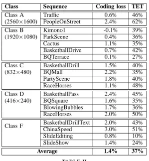
Table I gives the percentage of HEVC CUs where Assump-tion 1 is true for several test sequences. The experimental setting used to obtain these results is described in Section IV-A (we used the random access configuration here and a threshold

T = 1 in the fusion algorithm). We can see from Table I

Class Sequence _{22 27}QP_{32 37} Class A (2560×1600) Traffic 67 74 82 89 PeopleOnStreet 66 70 75 80 Class B (1920×1080) Kimono1 73 78 80 79 ParkScene 66 71 75 77 Cactus 66 70 75 78 BasketballDrive 71 75 78 79 BQTerrace 63 68 72 73 Class C (832×480) BasketballDrill 69 73 80 87 BQMall 70 75 81 87 PartyScene 61 69 75 83 RaceHorses 69 75 81 87 Class D (416×240) BasketballPass 71 74 80 86 BQSquare 54 69 77 85 BlowingBubbles 64 74 82 90 RaceHorses 70 74 81 87 Class F BasketballDrillText 68 70 77 83 ChinaSpeed 72 75 80 86 SlideEditing 86 87 89 93 SlideShow 85 88 90 93 TABLE I

PERCENTAGE OFHEVC CUS WHEREASSUMPTION1IS TRUE

that the assumption seems reasonable. As the QP increases, the decoded AVC video becomes smoother and hence, the HEVC encoder uses larger CUs (and consequently less splits) to code the frames. As the HEVC quadtree becomes coarser,

the assumption failures are bound to decrease as can be seen in Table I. There are indeed some cases where this assumption is false (i.e. an HEVC CU is more partitioned than its collocated CU in the fused AVC quadtree). For instance, AVC compression artifacts may exist in the AVC decoded video. These may lead the HEVC encoder to split the corresponding CUs to account for these artifacts, non-existent at the AVC encoding stage. However, since these cases are rare judging from Table I, if the HEVC quadtree is forced to be limited to the fused AVC one, significant execution time savings can be obtained with a reasonable loss in coding efficiency.

This is precisely what the proposed method does. After fusing the AVC coding structure of F , when coding an HEVC CU in F , the limitation shown in Figure 5 is forced so that the CU cannot be more partitioned than its collocated CU in the fusion map (CUcol).

CUcol Allowed HEVC CU partitions

Fig. 5. Quadtree limitation algorithm

Our limitation algorithm is the following: if CUcol is split or coded in an N×N partition, the HEVC encoder tests all PU sizes and also tries splitting the CU into four smaller CUs, as normally done: No limitation is applied in this case. If CUcolis partitioned in 2N×2N, only 2N×2N modes are tested in HEVC (Merge 2N×2N, Inter 2N×2N, Intra 2N×2N) and the CU split recursion is stopped: the PU is coincident with the CU. If CUcolis partitioned in any way other than 2N×2N,

only the 2N×2N modes and the partition of CUcol into PUs with the same shape as CUcol are tested in HEVC and here also, the split recursion is stopped. Note that the proposed quadtree limitation algorithm is not applied for I slices: the coding of these slices remains unchanged in our method. The reason is that, on one hand, the coding time of I slices is only a very small fraction of the coding time of a GOP, so little can be gained in terms of execution time reduction; on the other hand, reducing quality of the I slices may have a huge impact on the quality of all slices in the GOP, since the latter are predicted from the former. This intuitive reasoning is fully supported by experimental results, as shown in Section IV-C. Also note that the limitation algorithm is inherently different than MVVD, presented in [18], because our method ultimately tries to make the HEVC quadtree similar to what would have been the quadtree coding structure of the AVC frame if CUs and PUs were used instead of MBs, whereas MVVD only analyzes the scene complexity using MVs and offers accordingly a different subset of possible partitions at a time.

C. Motion vector reuse

In the integer motion estimation of HM-13.0, the starting point for the diamond search is the MVP. However, a better starting point can make the search converge more quickly to the best vector. For instance, in Figure 2, choosing directly the green point as starting position instead of the red point (MVP) allows avoiding one whole diamond search iteration. In this paper, we propose to change the starting position of the integer motion estimation in HM-13.0: the MVP, as well as all the MVs covered by the currently tested HEVC PU in the fused AVC quadtree are tested by RDO and the one minimizing an RD cost is selected as the best starting position for the diamond search.

IV. EXPERIMENTAL RESULTS A. Experimental setting

The JM-18.6 [26] reference software for AVC is used to encode the original video. We limit our scenario to the case where the AVC encoder is properly designed and run using a reasonable configuration of parameters. In particular, since our method relies on motion vectors extracted from the AVC bitstream, we assume that the motion estimation process was run with a reasonably effective configuration. We acknowledge the fact that it would be very interesting, for practical applications, to test the proposed transcoder in the case of a poorly designed AVC encoding step. This study would require much more space and will be the subject of future works; we only mention here that in principle it is possible to detect a poorly estimated motion vector field, at least when the AVC encoded sequence has a reasonable PSNR1_{: it suffices to re-estimate MV with a well-configured} ME algorithm and to check if the result is coherent with the AVC motion vector field. However in the following we only consider the case of properly configured AVC encoder.

1_{We note that a bad motion vector field would affect the rate of the encoded}

sequence, not its PSNR that mainly depends on the quantization step.

After AVC decoding, the video is inputted to HM-13.0 where the proposed method is implemented. The trivial transcoder following the “Full Decode-Full Encode” approach is used as anchor for the results presented in this section.

The videos are encoded in two different configurations: a random access configuration (RA-MAIN) with a GOP size of 8 and an Intra period dependent on the sequence, and a low delay configuration (LD-P-MAIN) with four reference frames. Each configuration is used in both JM-18.6 and HM-13.0 encoders (the configuration files used: encoder JM RA B HE.cfg and

encoder random access main.cfg for random access, and en-coder JM LP HE.cfg and enen-coder lowdelay P main.cfg for

low delay, are included in the JM-18.6 and HM-13.0 packages respectively). The maximum and minimum CU sizes are set to 64×64 and 8×8 respectively in HM. Furthermore, the following options are all enabled in HM: fast search (during the motion estimation process), fast encoder decision (FEN), and fast decision for Merge RD cost (FDM). These options allow reducing the encoding execution time by exploiting local sequence characteristics. Hence, it is important to note that our method brings execution time savings over an already “fast” HM encoder.

Four QPs (22, 27, 32, 37) are selected to perform the sim-ulations. The same QP is used in both JM and HM encoders. Coding results have been evaluated using the Bjontegaard Delta Rate (BD-Rate) [27] metric. The rate considered in the computation of this metric is the one reported by the HM encoder. The PSNR considered is evaluated between the output of the HM decoder and the original uncompressed video. Tests have been performed on the sequences of the HEVC dataset. They are divided into six classes, based on either resolution or content (class F contains screen-content sequences with different resolutions). Ten seconds of video have been coded for each sequence. Note that results are not given for class E sequences in the random access configuration, nor for class A sequences in the low delay configuration because random access is not typically used to code video conferencing content (class E), and neither is low delay for high resolution sequences (class A). This is also why contributions to JCT-VC have never reported such values in their experimental results. Finally, the tests have been launched on a cluster of nine machines, four of which use an Intel Xeon X5670 processor with 24 cores while the remaining five use an Intel Xeon E5430 processor with 8 cores2_{. In order to obtain} stable results we obtained time measurements as averages over twenty repetitions.

B. Results of the proposed method

Tables II and III show the results of the proposed method in a random access (RA) and a low delay (LD) configuration respectively. In these tables, TET is the transcoder execution time, expressed as percent of the reference execution time in the case of the trivial (full decode-full encode) transcoder. The threshold T in the fusion algorithm is set empirically

2_{In order to reduce the dependency of our results from the hardware}

configuration, we also run the tests in a single PC scenario, obtaining results very close to those of the cluster.

to 0.5 as this value offers a good tradeoff between execution time savings and coding losses. The method achieves 63% (resp. 56%) execution time savings with an average coding loss of 1.4% (resp. 3.7%) in the RA (resp. LD) configuration. For some screen content sequences, such as SlideEditing and SlideShow, results in LD configuration may be improved by using a smaller threshold: with T = 0, the coding loss passes from 5.6% to 5.0% for SlideEditing and from 7.6% to 6.3% for SlideShow, with the same execution times.

Class Sequence Coding loss TET

Class A (2560×1600) Traffic 0.6% 46% PeopleOnStreet 2.4% 62% Class B (1920×1080) Kimono1 -0.1% 39% ParkScene 0.4% 36% Cactus 1.1% 35% BasketballDrive 0.7% 42% BQTerrace 0.1% 27% Class C (832×480) BasketballDrill 1.5% 40% BQMall 2.2% 35% PartyScene 1.8% 40% RaceHorses 1.1% 48% Class D (416×240) BasketballPass 2.4% 45% BQSquare 1.6% 35% BlowingBubbles 1.7% 36% RaceHorses 2.0% 50% Class F BasketballDrillText 2.0% 43% ChinaSpeed 3.0% 51% SlideEditing 0.8% 10% SlideShow 1.4% 24% Average 1.4% 37% TABLE II

CODING RESULTS AND TRANSCODER EXECUTION TIMES(TET)USING THE PROPOSEDFA+QTL+MVRMETHOD IN ARACONFIGURATION

Class Sequence Coding loss TET

Class B (1920×1080) Kimono1 0.6% 54% ParkScene 2.6% 44% Cactus 3.7% 57% BasketballDrive 2.1% 61% BQTerrace 2.5% 38% Class C (832×480) BasketballDrill 3.7% 50% BQMall 3.9% 49% PartyScene 3.9% 49% RaceHorses 3.2% 53% Class D (416×240) BasketballPass 4.0% 70% BQSquare 5.3% 47% BlowingBubbles 4.3% 66% RaceHorses 4.3% 66% Class E (1280×720) FourPeople 3.7% 26% Johnny 1.9% 22% KristenAndSara 2.3% 31% Class F BasketballDrillText 4.7% 55% ChinaSpeed 4.2% 68% SlideEditing 5.6% 11% SlideShow 7.7% 29% Average 3.7% 44% TABLE III

CODING RESULTS AND TRANSCODER EXECUTION TIMES(TET)USING THE PROPOSEDFA+QTL+MVRMETHOD IN ALDCONFIGURATION

Figure 6 shows, for the two configurations, the average coding results and execution times of the proposed method for various values of the threshold T used in the fusion

algorithm. Note that a threshold of 0 means that no fusion is performed on the AVC MBs. In the RA configuration, varying the threshold beyond 0.5 only increases the coding losses while maintaining the execution time around 38%. We have observed that in the RA configuration, the number of blocks after fusion varies only slightly with the threshold. This explains the little variation in the execution time in Figure 6(a), mainly due to to more or less concurrent CPU load of the machines. For the LD configuration however, we can see that as the threshold increases, the execution times decrease and the coding losses increase. We observed that is due to the fact that in this configuration, the threshold value has a larger impact on the number of blocks after fusion. Hence, an advantage of the proposed method is that in a LD configuration, a new coding loss / execution time savings trade-off can be achieved, depending on the desired application, by simply varying a single threshold value.

1 2 3 4 5 30 35 40 45 50 0 0.5 1 1.5 2 3 5 10 Coding loss Execution time (a) RA 0 5 10 15 20 30 35 40 45 50 0 0.5 1 1.5 2 3 5 10 Coding loss Execution time (b) LD

Fig. 6. Evolution of the coding losses and execution times with the threshold

C. Results of some variants of the proposed method

In order to single out the contributions of the different tools that constitute our technique, we implemented some variation of the proposed method. In a first variation, referred to as FA+QTL, we perform the fusion algorithm and the quadtree limitation, but the motion estimation step is unchanged, that is we use the default motion estimation of the HM software. In opposition to this variant, we refer to the main method (described in Section III) as FA+QTL+MVR. We also consider a version of our transcoder where the quadtree limitation is also performed on Intra slices. This version is referred to as FA+QTLI. Finally, since the main contribution of our technique lies in the fusion and the quad-tree limitation, we also consider a version of the proposed method where these FA and QTL are turned off and only motion vector reuse, as described in Sec. III-C, is employed. This allows us estimating the actual contribution of the most innovative part of the proposed technique. We refer to this last method as MVR.

Variant Coding loss TET

FA+QTL 2.2% 42%

FA+QTLI 4.5% 42%

TABLE IV

AVERAGE CODING RESULTS AND EXECUTION TIMES(TET)OBTAINED USING VARIANTS OF THE PROPOSED METHOD IN ARACONFIGURATION

The results for the first two variants are shown in Table IV for the RA configuration (average coding loss and average

ex-ecution time on the set of test sequences). The same threshold

T = 0.5 as for the main method is used in these variants.

Comparing with the average results of FA+QTL+MVR in Table II, we observe that the MVR technique improves both the execution time (from 42% to 37%) and the coding loss (from 2.2% to 1.4%). We explain this behavior as follows. First, we observed that the FQ+QTL+MVR scheme converges more quickly to the best integer motion vector. On average, we measured a reduction of total number of tested motion vectors of 7% in the RA configuration compared to FA+QTL. In addition, the MVR scheme also allows to converge to a better (RD-wise) final point than what would have been found in the diamond search which uses systematically the MVP as its starting point.

Comparing FA+QTL and FQ+QTLI, we can see that by not applying QTL on I slices (as done in the main method), the coding losses are halved while maintaining the same execution time. This is because, on one hand, I slices only represent, on average, 3% of the total number of slices coded for each sequence and moreover the encoding time of I slices is already small enough to begin with due to the lack of motion estimation. Hence, applying the QTL on these slices does not significatevely reduce the total transcoding time. On the other hand, QTL may reduce the quality of the I slices, and this have a large impact on all the slices of a GOP. This explains why not applying QTL on I slices the reduces the coding losses.

As far as the MVR method is concerned, since no fusion nor quad-tree limitation are performed, it risks to be not very effective: several macroblock may correspond to a single HEVC prediction unit, and so several motion vectors have to undergo the RDO test in order to select the new starting point of the diamond search. In other words, without fusion and quad-tree limitation, MVR may lead to test many MVs. These intuitions have been confirmed by our experiments. In the same experimental conditions as FA+QTL+MVR, the MVR technique leads to a small coding rate increase, but with no transcoding execution time reduction (actually we observed a small transcoding time increase of 2 % with respect to FD-FE). We conclude that MVR works well only when it is used jointly with other methods that effectively reduce the number of MVs to be tested, keeping the “good ones” in the bundle. FA+QTL is effective in this task, since when used with MVR the global performance is improved. On the other hand, this experiment also proved that the most relevant part of the proposed technique is the novel FA+QTL rather than the well known MVR.

Finally consider a further variant of the proposed method with a different MVR scheme (FA and QTL are unchanged), referred to as FA+QTL+MVR2. In this variant, after selecting the best starting position out of the MVP and the AVC MVs covered by the current PU, the diamond search is not performed. The best starting position is directly set as the MV of the PU, so we may expect further time savings but possible coding loss. We also observe that this motion vector reuse technique corresponds to the one used in [18]. The results, in both RA and LD configurations and for a threshold T = 0.5, are given in Tables V and VI.

We observe that FA+QTL+MVR2 is faster than

Class Sequence Coding loss TET

Class A (2560×1600) Traffic 0.9% 42% PeopleOnStreet 2.7% 57% Class B (1920×1080) Kimono1 0.9% 33% ParkScene 0.5% 39% Cactus 1.1% 30% BasketballDrive 0.8% 35% BQTerrace 0.4% 29% Class C (832×480) BasketballDrill 1.6% 33% BQMall 2.2% 34% PartyScene 1.7% 41% RaceHorses 1.9% 38% Class D (416×240) BasketballPass 2.4% 44% BQSquare 1.6% 39% BlowingBubbles 1.8% 35% RaceHorses 2.5% 45% Class F BasketballDrillText 2.0% 40% ChinaSpeed 3.9% 41% SlideEditing 1.1% 10% SlideShow 2.8% 23% Average 1.7% 35% TABLE V

CODING RESULTS AND TRANSCODER EXECUTION TIMES(TET)USING THEFA+QTL+MVR2METHOD IN ARACONFIGURATION

Class Sequence Coding loss TET

Class B (1920×1080) Kimono1 1.1% 44% ParkScene 3.5% 44% Cactus 4.1% 45% BasketballDrive 2.8% 42% BQTerrace 3.4% 39% Class C (832×480) BasketballDrill 4.3% 34% BQMall 4.3% 38% PartyScene 4.6% 52% RaceHorses 4.4% 39% Class D (416×240) BasketballPass 4.7% 45% BQSquare 5.9% 49% BlowingBubbles 4.8% 55% RaceHorses 5.6% 41% Class E (1280×720) FourPeople 4.3% 22% Johnny 2.0% 17% KristenAndSara 2.6% 26% Class F BasketballDrillText 6.0% 38% ChinaSpeed 6.6% 39% SlideEditing 10.1% 9% SlideShow 10.4% 18% Average 4.8% 34% TABLE VI

CODING RESULTS AND TRANSCODER EXECUTION TIMES(TET)USING THEFA+QTL+MVR2METHOD IN ALDCONFIGURATION

FA+QTL+MVR (35% vs. 37% TET in RA and 34% vs. 44% TET in LD) but also higher coding losses (1.7% vs. 1.4% in RA and 4.8% vs 3.7% in LD). In order to explain this, we have measured that with the FA+QTL+MVR2 variant, the number of tested motion vectors is significantly reduced (by 98% in the RA configuration) compared to FA+QTL+MVR, thus explaining the time saving. However, without the refinement, the estimated motion vector will not be as accurate, thus incurring the additional coding losses.

D. Comparison with state-of-the-art methods

We have compared our proposed method to other re-cent transcoding techniques found in the literature. Existing

methods are not consistently tested over all the HEVC test sequences and configurations. Hence, we have evaluated our method in the same testing conditions (coding configuration and sequences) as the ones used for each state-of-the-art technique in order to perform the most fair comparison.

1) Random access configuration: Under a random access

configuration, reference results are only available for three techniques: two of them, MVVD and LDF, have been proposed by Peixoto et al. in [20]; a third one has been introduced by Diaz-Onrubia et al. in [15]. Indeed, the results of the MVRT and RFA transcoders in this configuration are not available in the respective papers. Also, the presented results in [20] are limited to only two sequences: Kimono1 and ParkScene. Table VII compares our method to the two transcoders in [20]. A threshold of 0.5 was selected in the FA. We can see that

Sequence MVVD [20] LDF [20]

FA+QTL+MVR (T=0.5)

Loss TET Loss TET Loss TET

Kimono1 1.6% 52% 3% 40% -0.1% 39% ParkScene 4.3% 44% 4.2% 34% 0.4% 36%

Average 3% 48% 3.6% 37% 0.1% 37.5%

TABLE VII

COMPARISON BETWEEN OUR METHOD AND OTHER TRANSCODERS IN THE

RACONFIGURATION

in a random access configuration, our method is better than MVVD and LDF because it produces lower coding losses for lower (or similar) encoding execution times. Note that as in our method, MVVD and LDF also employ a threshold.

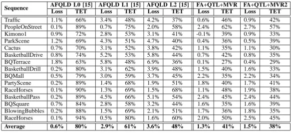
In Tab. VIII we show the comparison of the two variants of our method with AFQLD proposed in [15]. We first observe that AFQLD can be limited to level zero of the HEVC quadtree (L0, first and second column in Tab. VIII). In this case, the transcoding is not very different from the anchor: the TET is on the average 80% of FD-FE and the rate increase is small (0.6%). More interesting results are obtained when AFQLD is run up to levels 1 and 2 (L1 and L2 columns). However, compared to both the two version of our proposed algorithm, AFQLD has larger losses (around twice as ours) for smaller accelerations. We conclude that our method has globally better performance than AFQLD in RA configuration.

2) Low delay configuration: In a low delay configuration,

we can compare our method to four different transcoders: MVRT, MVVD, LDF, and RFA. For MVRT, results are presented in [18] for three sequences only: BasketballDrill, BQMall and RaceHorses (results are also given for the Vidyo sequence, but this sequence was not considered in our experiments because it is not in the current HEVC test set). For MVVD, results are provided for five sequences: BasketballDrill, BQMall, RaceHorses (in [18]), Kimono1 and ParkScene (in [20]). For LDF, results for only two sequences are given in [20]: Kimono1 and ParkScene. Finally, for RFA, results are given for classes B to E in [19]. Tables IX, X, XI, and XII compare our method to these four transcoders. Note that in those experiments, the threshold in the fusion algorithm was set with an aim to achieve the same average execution time as the technique to compare to, and thus be able to fairly compare coding losses. This, however, was not possible when

comparing with LDF and RFA (Tables XI and XII) because no threshold used in the fusion algorithm can match the TET values achieved with these two state-of-the-art transcoders. Indeed, varying the threshold only gives us a limited range of possible TET values as the TETs begin to saturate past a certain threshold value.

Sequence MVRT [18] FA+QTL+MVR (T=0.5)

Loss TET Loss TET

BasketballDrill 2.8% 71% 3.7% 50%

BQMall 3.2% 64% 3.9% 49%

RaceHorses 7.7% 56% 3.2% 53%

Average 4.6% 64% 3.6% 51%

TABLE IX

COMPARISON BETWEEN OUR METHOD ANDMVRTIN THELD

CONFIGURATION

Sequence MVVD [18], [20] FA+QTL+MVR (T=1.5)

Loss TET Loss TET

BasketballDrill 6.3% 39% 4.4% 46% BQMall 7.8% 43% 7.5% 45% RaceHorses 4.7% 56% 4.9% 54% Kimono1 3.0% 46% 1.7% 41% ParkScene 9.8% 34% 5.6% 39% Average 6.3% 44% 4.8% 45% TABLE X

COMPARISON BETWEEN OUR METHOD ANDMVVDIN THELD

CONFIGURATION

Sequence _LossLDF [20]_TET FA+QTL+MVR (T=1.5)_{Loss TET}

Kimono1 3.8% 37% 1.7% 41%

ParkScene 4.4% 33% 5.6% 39%

Average 4.1% 35% 3.7% 40%

TABLE XI

COMPARISON BETWEEN OUR METHOD ANDLDFIN THELD

CONFIGURATION

Sequence _LossRFA [19]_TET FA+QTL+MVR (T=0.5)_{Loss TET}

Kimono1 0.0% 50% 0.6% 54% ParkScene 0.6% 52% 2.6% 44% Cactus 0.1% 53% 3.7% 57% BQTerrace 2.1% 52% 2.5% 38% BasketballDrive 0.0% 50% 2.1% 61% FourPeople 0.2% 51% 3.7% 26% Johnny 4.3% 51% 1.9% 22% KristenAndSara 1.8% 51% 2.3% 31% RaceHorses (class C) 0.7% 50% 3.2% 53% BQMall 0.9% 52% 3.9% 49% PartyScene 3.5% 55% 3.9% 49% BasketballDrill 0.0% 51% 3.7% 50% RaceHorses (class D) 2.8% 50% 4.3% 66% BQSquare 4.6% 56% 5.3% 47% BlowingBubbles 4.4% 58% 4.3% 66% BasketballPass 1.9% 50% 4.0% 70% Average 1.7% 52% 3.2% 46% TABLE XII

COMPARISON BETWEEN OUR METHOD ANDRFAIN THELD

Sequence AFQLD L0 [15] AFQLD L1 [15] AFQLD L2 [15] FA+QTL+MVR FA+QTL+MVR2

Loss TET Loss TET Loss TET Loss TET Loss TET

Traffic 1.1% 66% 3.4% 48% 4.2% 37% 0.6% 46% 0.9% 42% PeopleOnStreet 0.1% 89% 0.7% 75% 2.0% 58% 2.4% 62% 2.7% 57% Kimono1 0.9% 72% 2.8% 53% 3.1% 41% -0.1% 39% 0.9% 33% ParkScene 1.2% 69% 4.3% 51% 4.7% 40% 0.4% 36% 0.5% 39% Cactus 0.7% 70% 3.1% 52% 3.8% 42% 1.1% 35% 1.1% 30% BasketballDrive 0.8% 74% 5.2% 53% 5.8% 44% 0.7% 42% 0.8% 35% BQTerrace 1.8% 63% 5.8% 48% 6.9% 36% 0.1% 27% 0.4% 29% BasketballDrill 0.2% 80% 3.1% 62% 3.9% 48% 1.5% 40% 1.6% 33% BQMall 0.5% 79% 3.0% 59% 3.7% 45% 2.2% 35% 2.2% 34% PartyScene 0.2% 89% 1.4% 68% 1.9% 51% 1.8% 40% 1.7% 41% RaceHorses 0.1% 90% 1.3% 69% 1.5% 68% 1.1% 48% 1.9% 38% BasketballPass 0.2% 89% 4.5% 66% 5.1% 54% 2.4% 45% 2.4% 44% BQSquare 0.7% 84% 2.8% 58% 3.2% 44% 1.6% 35% 1.6% 39% BlowingBubbles 0.2% 88% 1.5% 69% 2.1% 51% 1.7% 36% 1.8% 35% RaceHorses 0.1% 94% 0.5% 80% 1.6% 60% 2.0% 50% 2.5% 45% Average 0.6% 80% 2.9% 61% 3.6% 48% 1.3% 41% 1.5% 38% TABLE VIII

COMPARISON BETWEEN OUR METHOD ANDAFQLD [15]IN THERACONFIGURATION

.

Tables IX and X show that our method is better than MVRT and MVVD in a LD configuration, because our method produces lower coding losses at lower or comparable execution times. Table XI shows that our method produces a different coding loss / execution time trade-off than LDF. While LDF achieves more execution time savings, our method achieves lower coding losses. Two sequences may be insufficient to choose a clear winner between our method and LDF, and results on other sequences are unfortunately not reported in [20]. Our method is however better than LDF in a RA configuration as shown in Table VII.

Table XII shows that the RFA transcoder produces lower losses than our method (1.7% vs. 3.2%), but it is slower (RFA takes 12% more time in the average than ours). Therefore, we cannot conclude that our method is better than RFA, but that it provides a time-quality trade-off that is not achievable by RFA. This trade-off may be more valuable than the RFA’s one for two reasons. First, in LD configurations, the focus is typically on speed rather than on quality, otherwise one would choose an RA configuration and in this case our technique outperforms the state of the art; second, a typical application requiring a low delay is video-conference: for this kind of content (class E sequences), our techniques is much faster than RFA (26% of FD-FE vs. 51%, practically twice faster) with very close rate increases (2.6% vs. 2.3%).

In summary, our technique provides operational points that are not achievable by RFA; in addition, for the applications and the content where the LD configuration is more relevant, our technique is faster or much faster, with small (general content) to negligible (video conference content) rate losses. Our conclusion is that our technique is a valuable alternative to the state of the art, and that for video conference contents and applications (most relevant for LD), it seems more fit that the state of the art (twice faster with practically no losses).

Considering the RFA algorithm, we observe that it includes several steps: coding complexity region segmentation, adap-tive searching depth range decision of CTU, motion vector de-noise filter, motion vector clustering, adaptive minimum

searching depth and PU partitions selection, and optimization of motion vector predictor and search window size. This results in a complex algorithm which requires a one-frame preprocessing delay, whereas ours only has a one-CTU prepro-cessing delay (the encoding of the first CTU can be performed in parallel with the fusion of the second). Comparing the two techniques, ours is more adapted to the LD configurations in the sense that it requires only one CTU pre-processing delay, in opposition to one full image delay for RFA. Finally, in light of the various steps performed in RFA, we believe that our algorithm could be more easily adapted to hardware implementation, and that, in conclusion, it is suited to cases where RFA would be too slow or introduce too much delay.

FMD-FME [13] FMD-FME [14] FA+QTL+MVR

Loss TET Loss TET Loss TET

1.2% 60% 1.3% 59% 3.3% 45%

TABLE XIII

COMPARISON BETWEEN OUR METHOD ANDFMD-FME [13]AND[14]IN THELDCONFIGURATION,AVERAGE ONCLASSB, C & DSEQUENCES

In Tab. XIII we compare FA+QTL+MVR to FMD-FME [13] and [14]. For brevity, we report here only the average of the transcoding results, which were obtained on the sequences of classes B, C and D. As for the RFA case, we observe that the proposed method is faster than references even though it provides a larger coding rate. This result is relevant for low-delay application, where the processing time is arguably preeminent.

Finally, in Tab. XIV, we compare the proposed method with AFQLD in LD-P configuration. As for the RA case, we report the results of AFQLD for the three levels L0, L1 and L2. As for the RA configuration, the L0 level is not very relevant. For the L1 and L2 levels, we observe again that AFQLD has both larger BD-Rate losses and larger execution times than FA+QTL+MVR. Compared to FA+QTL+MVR2, AFQLD has similar or larger losses and definitely larger execution times. We conclude that also for the LD configuration the proposed

Sequence AFQLD L0 [15] AFQLD L1 [15] AFQLD L2 [15] FA+QTL+MVR FA+QTL+MVR2

Loss TET Loss TET Loss TET Loss TET Loss TET

Kimono1 0.4% 83% 2.6% 61% 3.0% 43% 0.6% 54% 1.1% 44% ParkScene 0.4% 81% 5.7% 57% 6.4% 44% 2.6% 44% 3.5% 44% Cactus 0.3% 79% 2.8% 65% 4.2% 50% 3.7% 57% 4.1% 45% BasketballDrive 0.1% 86% 3.6% 63% 4.5% 50% 2.1% 61% 2.8% 42% BQTerrace 0.4% 76% 9.5% 55% 10.2% 44% 2.5% 38% 3.4% 39% BasketballDrill 0.0% 86% 1.7% 69% 3.3% 52% 3.7% 50% 4.3% 34% BQMall 0.2% 88% 1.1% 75% 2.4% 53% 3.9% 49% 4.3% 38% PartyScene 0.0% 93% 0.5% 79% 1.5% 60% 3.9% 49% 4.6% 52% RaceHorses 0.0% 93% 0.6% 79% 1.3% 63% 3.2% 53% 4.4% 39% BasketballPass 0.0% 92% 1.3% 75% 2.2% 61% 4.0% 70% 4.7% 45% BQSquare 0.1% 93% 2.3% 70% 3.0% 56% 5.3% 47% 5.9% 49% BlowingBubbles 0.0% 94% 0.3% 82% 1.5% 61% 4.3% 66% 4.8% 55% RaceHorses 0.1% 94% 0.5% 81% 1.3% 66% 4.3% 66% 5.6% 41% FourPeople 1.7% 52% 7.2% 39% 7.5% 30% 3.7% 26% 4.3% 22% Johnny 5.6% 61% 13.4% 29% 11.9% 23% 1.9% 22% 2.0% 17% KristenAndSara 3.7% 47% 9.4% 36% 10.0% 27% 2.3% 31% 2.6% 26% Average 0.8% 81% 3.9% 63% 4.6% 49% 3.3% 48% 3.9% 39% TABLE XIV

COMPARISON BETWEEN OUR METHOD ANDAFQLD [15]IN THELDCONFIGURATION

algorithms outperform AFQLD. V. CONCLUSION

In this paper, we have presented a novel AVC to HEVC transcoder based on quadtree limitation. AVC blocks are first fused using a fusion algorithm in order to translate the AVC coding structure into one comparable to that of HEVC. The HEVC quadtree is then limited to the fused AVC one. The method is coupled with a motion vector reuse scheme to further bring execution time savings. The proposed method brings 63% execution time savings with only a 1.4% coding loss in a random access configuration. It offers also other advantages: the fusion algorithm can be executed in parallel on multiple CTUs at once, hence allowing an efficient hardware implementation of the method. Also, the trade-off between coding losses and execution time savings can be fine-tuned using a single threshold value. Compared to other state-of-the-art transcoders, the proposed method is better in a random access configuration. In a low delay configuration, it offers better or similar performance, especially on video conferencing content at which low delay coding configurations are typically aimed.

The limitations of the present work lie in the following issues. First, only a subset of the available information of the H.264/AVC stream was exploited in our technique: in the future, additional information from the AVC bitstream can be used to further increase execution time savings. The energy of the residuals, the number of non-zero DCT coefficients, and the Intra directions are some examples of such AVC information. These can be used to further reduce execution time in other parts of the HEVC encoding process, such as Intra tests, transform size selection, and entropy coding. Second, the selection of the optimal threshold value T = 1 has been performed on a quite complete test set, but for a specific content or application other values may give better results. An adaptive threshold selection technique will be investigated in the future. Third, we did not take into account the effects of a bad configuration of the H.264 encoder, neither

its specific artifacts. Finally, we have not considered the effect of transmission on lossy channels. These relevant issues will be the subject of future works.

VI. ACKNOWLEDGEMENTS

This work has been performed in the framework of the Eurostars-Eureka Project E! 8307 - Transcoders Of the Future TeleVision (TOFuTV).

REFERENCES

[1] G. Sullivan, J. Ohm, W.-J. Han, and T. Wiegand, “Overview of the High Efficiency Video Coding (HEVC) standard,” IEEE Transactions on

Circuits and Systems for Video Technology, vol. 22, no. 12, pp. 1649–

1668, Dec 2012.

[2] T. Wiegand, G. Sullivan, G. Bjontegaard, and A. Luthra, “Overview of the H.264/AVC video coding standard,” IEEE Transactions on Circuits

and Systems for Video Technology, vol. 13, no. 7, pp. 560–576, July

2003.

[3] C. Simpson, “Samsung’s Galaxy S4 has a next-gen video codec,” PC

world, March 2013. [Online]. Available: http://bit.ly/1lq95u5

[4] I. Ahmad, X. Wei, Y. Sun, and Y.-Q. Zhang, “Video transcoding: an overview of various techniques and research issues,” IEEE Transactions

on Multimedia, vol. 7, no. 5, pp. 793–804, Oct 2005.

[5] J. Xin, C.-W. Lin, and M.-T. Sun, “Digital video transcoding,”

Proceed-ings of the IEEE, vol. 93, no. 1, pp. 84–97, Jan 2005.

[6] A. Vetro, C. Christopoulos, and H. Sun, “Video transcoding architec-tures and techniques: an overview,” IEEE Signal Processing Magazine, vol. 20, no. 2, pp. 18–29, Mar 2003.

[7] R. Garrido-Cantos, J. De Cock, J. L. Mart´ınez, S. Van Leuven, and A. Garrido, “Video transcoding for mobile digital television,”

Telecom-munication Systems, vol. 52, no. 4, pp. 2655–2666, 2013.

[8] S. Kaware and S. Jagtap, “A survey: Heterogeneous video transcoder for H.264/AVC to HEVC,” in International Conference on Pervasive

Computing (ICPC), 2015.

[9] W.-J. Han, J. Min, I.-K. Kim, E. Alshina, A. Alshin, T. Lee, J. Chen, V. Seregin, S. Lee, Y. M. Hong, M.-S. Cheon, N. Shlyakhov, K. McCann, T. Davies, and J.-H. Park, “Improved video compression efficiency through flexible unit representation and corresponding extension of coding tools,” IEEE Transactions on Circuits and Systems for Video

Technology, vol. 20, no. 12, pp. 1709 –1720, December 2010.

[10] F. Bossen. HM-13.0 reference software. [Online]. Available: https://hevc.hhi.fraunhofer.de/trac/hevc/browser/tags/HM-13.0

[11] P. Xing, Y. Tian, X. Zhang, Y. Wang, and T. Huang, “A coding unit classification based AVC-to-HEVC transcoding with background modeling for surveillance videos,” in Visual Communications and Image

[12] E. Peixoto, B. Macchiavello, E. M. Hung, A. Zaghetto, T. Shanableh, and E. Izquierdo, “An H.264/AVC to HEVC video transcoder based on mode mapping,” in Image Processing (ICIP), 2013 20th IEEE International

Conference on. IEEE, 2013, pp. 1972–1976.

[13] Z. Chen, C. Tseng, and P. Chang, “Fast inter prediction for H.264 to HEVC transcoding,” in Proc. of the 3rd International Conference in

Multimedia Technology (ICMT). Guangzhou, China: Atlantis Press, nov 2013, pp. 1301–1308.

[14] Z. Chen, J. Fang, T. Liao, and P. Chang, “Efficient PU mode decision and motion estimation for H.264/AVC to HEVC transcoder,” Signal and

Image Processing: An International Journal, vol. 5, no. 2, pp. 81–93,

apr 2014, dOI: 10.5121/sipij.2014.5208.

[15] A. J. Diaz-Honrubia, J. L. Martinez, P. Cuenca, J. A. Gamez, and J. M. Puerta, “Adaptive fast quadtree level decision algorithm for h. 264/hevc video transcoding,” IEEE Transactions on Circuits and Systems for Video

Technology, vol. 26, no. 1, pp. 154–168, jan 2016.

[16] T. Shen, Y. Lu, Z. Wen, L. Zou, Y. Chen, and J. Wen, “Ultra fast H.264/AVC to HEVC transcoder,” in Data Compression Conference

(DCC), March 2013, pp. 241–250.

[17] D. Zhang, B. Li, J. Xu, and H. Li, “Fast transcoding from H.264 AVC to High Efficiency Video Coding,” in IEEE International Conference on

Multimedia and Expo (ICME), July 2012, pp. 651–656.

[18] E. Peixoto and E. Izquierdo, “A complexity-scalable transcoder from H.264/AVC to the new HEVC codec,” in 19th IEEE International

Conference on Image Processing (ICIP), Sept 2012, pp. 737–740.

[19] W. Jiang, Y. Chen, and X. Tian, “Fast transcoding from H.264 to HEVC based on region feature analysis,” Multimedia Tools and Applications, pp. 1–22, 2013.

[20] E. Peixoto, T. Shanableh, and E. Izquierdo, “H.264/AVC to HEVC video transcoder based on dynamic thresholding and content modeling,” IEEE

Transactions on Circuits and Systems for Video Technology, vol. 24,

no. 1, pp. 99–112, Jan 2014.

[21] E. Mora, J. Jung, M. Cagnazzo, and B. Pesquet-Popescu, “Initialization, limitation, and predictive coding of the depth and texture quadtree in 3D-HEVC,” IEEE Transactions on Circuits and Systems for Video

Technology, vol. 24, no. 9, pp. 1554–1565, Sept 2014.

[22] P. Helle, S. Oudin, B. Bross, D. Marpe, M. Bici, K. Ugur, J. Jung, G. Clare, and T. Wiegand, “Block merging for quadtree-based partition-ing in HEVC,” IEEE Transactions on Circuits and Systems for Video

Technology, vol. 22, no. 12, pp. 1720–1731, dec 2012.

[23] X. Li, R. Wang, W. Wang, Z. Wang, and S. Dong, “Fast motion estimation methods for HEVC,” in IEEE International Symposium on

Broadband Multimedia Systems and Broadcasting (BMSB), June 2014,

pp. 1–4.

[24] A. J. Diaz-Honrubia, J. L. Martinez, and P. Cuenca, “Multiple reference frame transcoding from H.264/AVC to HEVC,” in Proc. Int. Conf.

Multimedia Model. (MMM), Dublin, Ireland, jan 2014, pp. 593–604.

[25] A. J. Diaz-Honrubia, J. L. Martinez, J. M. Puerta, J. A. G´amez, J. De Cock, and P. Cuenca, “Fast quadtree level decision algorithm for H.264/HEVC transcoder,” in Image Processing (ICIP), 2014 IEEE

International Conference on. IEEE, 2014, pp. 2497–2501.

[26] ITU-T. JM-18.6 reference software. [Online]. Available: http://iphome.hhi.de/suehring/tml/download/

[27] G. Bjontegaard, “Calculation of average PSNR differences between RD-curves,” in VCEG Meeting, Austin, USA, April 2001.