Perceptual Texture Similarity for Machine Intelligence Applications

HAL Id: hal-01645011

https://hal.archives-ouvertes.fr/hal-01645011

Submitted on 22 Nov 2017

HAL is a multi-disciplinary open access

archive for the deposit and dissemination of

sci-entific research documents, whether they are

pub-lished or not. The documents may come from

teaching and research institutions in France or

abroad, or from public or private research centers.

L’archive ouverte pluridisciplinaire HAL, est

destinée au dépôt et à la diffusion de documents

scientifiques de niveau recherche, publiés ou non,

émanant des établissements d’enseignement et de

recherche français ou étrangers, des laboratoires

publics ou privés.

Applications

Karam Naser, Vincent Ricordel, Patrick Le Callet

To cite this version:

Karam Naser, Vincent Ricordel, Patrick Le Callet. Perceptual Texture Similarity for Machine

In-telligence Applications. Visual Content Indexing and Retrieval with Psycho-Visual Models, 2017.

�hal-01645011�

Abstract Textures are homogeneous visual phenomena commonly appearing in the visual scene. They are usually characterized by randomness with some stationar-ity. They have been well studied in different domains, such as neuroscience, vision science and computer vision, and showed an excellent performance in many applica-tions for machine intelligence. This book chapter focuses on a special analysis task of textures for expressing texture similarity. This is quite a challenging task, because the similarity highly deviates from point-wise comparison. Texture similarity is key tool for many machine intelligence applications, such as recognition, classification, synthesis and etc. The chapter review the theories of texture perception, and pro-vides a survey about the up-to-date approaches for both static and dynamic textures similarity. The chapter focuses also on the special application of texture similarity in image and video compression, providing the state of the art and prospects

1 Introduction

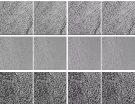
Textures are fundamental part of the visual scene. They are random structures often characterized by homogeneous properties, such as color, orientation, regularity and etc. They can appear both as static or dynamic, where static textures are limited to spatial domain (like texture images shown in Fig. 1), while dynamic textures involves both the spatial and temporal domain Fig. 2.

Research on texture perception and analysis is known since quite a long time. There exist many approaches to model the human perception of textures, and also many tools to characterize texture. They have been used in several applications such

University of Nantes, LS2N UMR CNRS 6004 Polytech Nantes Rue Christian Pauc BP 50609 44306 Nantes Cedex 3, France,

e-mail: {karam.naser; vincent.ricordel; patrick.le-callet}@univ-nantes.fr

Fig. 1: Example of texture images from VisTex Dataset

Fig. 2: Example of dynamic textures from DynTex Dataset [1]. First row represents the first frame, and next rows are frames after respectively 2 seconds

as scene analysis and understanding, multimedia content recognition and retrieval, saliency estimation and image/video compression systems.

There exists a large body of reviews on texture analysis and perception. For ex-ample, the review of Landy [2][3] as well as the one from Rosenholtz [4] give a detailed overview of texture perception. Besides, the review of Tuceryan et al. in [5] covers most aspects of texture analysis for computer vision applications, such as material inspection, medical image analysis, texture synthesis and segmentation. On the other hand, the book Haindl et al. [6] gives an excellent review about modeling both static and dynamic textures. A long with this, there are also other reviews that cover certain scope of texture analysis and perception, such as [7, 8, 9, 10, 11].

This chapter reviews an important aspect of texture analysis, which is texture similarity. This is because it is the fundamental tool for different machine intelli-gence applications. Unlike most of the other reviews, this covers both static and dynamic textures. A special focus is put on the use of texture similarity concept in data compression.

2 What is Texture

Linguistically, the word texture significantly deviates from the technical meaning in computer vision and image processing. According to Oxford dictionary [12], the word refers to one of the followings:

1. The way a surface, substance or piece of cloth feels when you touch it 2. The way food or drink tastes or feels in your mouth

3. The way that different parts of a piece of music or literature are combined to create a final impression

However, technically, the visual texture has many other definitions, for example: • We may regard texture as what constitute a macroscopic region. Its structure is simply attributed to pre-attentive patterns in which elements or primitives are arranged according to placement order [13].

• Texture refers to the arrangement of the basic constituents of a material. In a digital image, texture is depicted by spatial interrelationships between, and/or spatial arrangement of the image pixels [14].

• Texture is a property that is statistically defined. A uniformly textured region might be described as predominantly vertically oriented, predominantly small in scale, wavy, stubbly, like wood grain or like water [2].

• We regard image texture as a two-dimensional phenomenon characterized by two orthogonal properties: spatial structure (pattern) and contrast (the amount of local image structure) [15].

• Images of real objects often do not exhibit regions of uniform and smooth inten-sities, but variations of intensities with certain repeated structures or patterns, referred to as visual texture [16].

• Textures, in turn, are characterized by the fact that the local dependencies be-tween pixels are location invariant. Hence the neighborhood system and the ac-companying conditional probabilities do not differ (much) between various im-age loci, resulting in a stochastic pattern or texture [17].

• Texture images can be seen as a set of basic repetitive primitives characterized by their spatial homogeneity [18].

• Texture images are specially homogeneous and consist of repeated elements, of-ten subject to some randomization in their location, size, color, orientation [19]. • Texture refers to class of imagery that can be characterized as a portion of infinite

• Textures are usually referred to as visual or tactile surfaces composed of re-peating patterns, such as a fabric [7].

The above definitions cover mostly the static textures, or spatial textures. How-ever, the dynamic textures, unlike static ones, have no strict definition. The naming terminology changes a lot in the literature. The following names and definitions are summary of what’s defined in research:

• Temporal Textures:

1. They are class of image motions, common in scene of natural environment, that is characterized by structural or statistical self similarity [21]

2. They are objects possessing characteristic motion with indeterminate spatial and temporal extent[22]

3. They are textures evolving over time and their motion are characterized by temporal periodicity or regularity[23].

• Dynamic Textures:

1. They are sequence of images of moving scene that exhibit certain stationarity properties in time [24][9].

2. Dynamic textures (DT) are video sequences of non-rigid dynamical objects that constantly change their shape and appearance over time[25].

3. Dynamic texture is used with reference to image sequences of various natural processes that exhibit stochastic dynamics [26].

4. Dynamic, or temporal, texture is a spatially repetitive, time-varying visual pattern that forms an image sequence with certain temporal stationarity [27]. 5. Dynamic textures are spatially and temporally repetitive patterns like trees

waving in the wind, water flows, fire, smoke phenomena, rotational motions [28].

• Spacetime Textures:

1. The term spacetime texture is taken to refer to patterns in visual spacetime that primarily are characterized by the aggregate dynamic properties of elements or local measurements accumulated over a region of spatiotemporal support, rather than in terms of the dynamics of individual constituents [29].

• Motion Texture:

1. Motion textures designate video contents similar to those named temporal or dynamic textures. Mostly, they refer to dynamic video contents displayed by natural scene elements such as flowing rivers, wavy water, falling snow, rising bubbles, spurting foun- tains, expanding smoke, blowing foliage or grass, and swaying flame [30].

• Texture Movie:

1. Texture movies are obtained by filming a static texture with a moving camera [31].

arity properties with regularity exhibiting in both time and space [33]. It is worth also mentioning that in the context of component based video coding, the textures are usually considered as details irrelevant regions, or more specifically, the region which is not noticed by the observers when it is synthesized [34] [35] [36].

As seen, there is no universal definition of the visual phenomena of textures, and there is a large dispute between static and dynamic textures. Thus, for this work, we consider the visual texture as:

A visual phenomenon, that covers both spatial and temporal textures. Where spa-tial textures refer to us as homogeneous regions of the scene composed of small ele-ments (texels) arranged in a certain order, they might exhibit simple motion such as translation, rotation and zooming. In the other hand, temporal textures are textures that evolve over time, allowing both motion and deformation, with certain station-arity in space and time.

3 Studies on Texture perception

3.1 Static Texture Perception

Static texture perception has attracted the attention of researchers since decades. There exists a bunch of research papers dealing with this problem. Most of the studies attempt to understand how two textures can be visually discriminated, in an effortless cognitive action known as pre-attentive texture segregation.

Julesz extensively studied this problem. In his initial work in [37, 38], he posed a question if the human visual system is able to discriminate textures, generated by a statistical model, based on the kth_{order statistics, and what is the minimum value}

of k that beyond which the pre-attentive discrimination is not possible any more. The order of statistics refers to the probability distribution of the of pixels values, in which the 1st _{order measures how often a pixel has certain color (or luminance}

value), while the 2nd_{order measures the probability of obtaining a combination of}

two pixels (with a given distance) colors, and the same can be generalized for higher order statistics.

First, Julesz conjectured that the pre-attentive textures generated side-by-side, having identical 2nd _{order statistics but different 3}rd _{order and higher, cannot be}

discriminated without scrutiny. In other words, textures having difference in the 1st

and/or 2nd _{order statistics can be easily discriminated. This can be easily verified}

with the textures given in Fig. 3. The textures are generated by a small texture ele-ment (letter L) in three manners. First, to have different the 1st_{order statistics, where}

the probability of black and while pixels is altered in Fig. 3a (different sizes of L). Second, to have difference in 2nd_{order statistics (with identical 1}st _{order statistics)}

by relatively rotating one texture to the other. Third, to have difference in 3rd _order

statistics (with identical 1st_{and 2nd}st_{order statistics) by using a mirror copy of the}

texture element (L). One can easily observe that conjecture holds here, as we just observe the differences pre-attentively when the difference is below the 2nd _order

statistics. Several other examples can be found in [38] to support this conjecture.

(a) different 1st_{order statistics (b) different 2}nd_{order statistics (c) different 3}rd_{order statistics}

Fig. 3: Examples of pre-attentive textures discrimination. Each image is composed of two textures side-by-side. (a) and (b) are easily distinguishable textures because of the difference in the 1st _{and the 2}nd_{order statistics (resp.), while (c), which has}

identical 1st_{and the 2}nd_{but different 3}rd_{order statistics, is not. Images were copied}

from [39, 37].

However, it was realized then it is possible to generate other textures having iden-tical 3rd _{order statistics, and yet pre-attentively discriminable [40]. This is shown in}

Fig. 4, in which the left texture has an even number of black blocks in each of its 2x2 squares, whereas the left one has an odd number. This lead to the modified Julesz conjecture and the introduction of the texton theory [39]. The theory pro-poses that the pre-attentive texture discrimination system cannot globally process third or higher order statistics, and that discrimination is the results of few local conspicuous features, called textons. This has been previously highlighted by Beck [41], where he proposed that the descrimination is a result of difference in first order statistics of local local features (color, brightness, size and etc.).

On the other side, with the evolution of the neurophysiological studies in the vision science, the research on texture perception has envovled, and several neu-ral models of human visual system (HVS) were proposed. The functionality of the visual receptive field in [42], has shown that HVS, or more specifically the visual

Fig. 4: Example of 2 textures (side-by-side) having identical 3rd_{order statistics, yet}

pre-attentively distinguishable.

cortex, analysis the input signal by a set of narrow frequency channels, resembling to some extent the Gaborian filtering [43]. According, different models of texture dis-crimination have been developped, based on Gabor filtering [44, 45], or difference of offset Gaussians [46], etc. These models are generally performing the following steps:

1. Multi-channel filtering 2. Non linearity stage

3. Statistics in the resulting space

The texture perception models based on the multi-channel filtering approach is known as back-pocket model (according to Landy [2, 3]). This model, shown in Fig. 5, consists of three fundamental stages: linear, non-linear, linear (LNL). The first linear stage accounts for the linear filtering of the multi-channel approach. This is followed then by a non-linear stage, which is often rectification. This stage is required to avoid the problem of equal luminance value which will on average cancel out the response of the filters (as the filters are usually with zero mean). The last stage refers to us as pooling, where a simple sum can give an attribute for a region such that it can be easily segmented or attached to neighboring region. The LNL model is also occasionally called filter-rectify-filter (FRF) as how is performs the segregation [4].

Fig. 5: The Back-pocket perceptual texture segregation model [3]

.

3.2 Motion Perception

Texture videos, as compared to texture images, add the temporal dimension to the perceptual space. Thus, it is important to include the temporal properties of the visual system in order to understand its perception. For this reason, the subsection provides an overview of studies on motion perception.

The main unit responsible for motion perception is the visual cortex [47]. Gen-erally, the functional units of the visual cortex, which are responsible for motion processing, can be grouped into two stages:

1. Motion Detectors

The motion detectors are the visual neurons whose firing rate increases when an object moves in front of the eye, especially within the foveal region. Several studies have shown that the primary visual cortex area (V1) is place where the motion detection happens [48, 49, 50, 51]. In V1, simple cells neurons are often modeled as a spatio-temporal filter that are tuned to a specific spatial frequency and orientation and speed. On the other hand, complex cells perform some non-linearity on top of the simple cells (half/full wave rectification and etc.). The neurons of V1 are only responsive to signal having the preferred frequency-orientation-speed combination. Thus, there is still a lack of the motion integration from all neurons. Besides, the filter response cannot cope with the aperture prob-lem. As shown in Fig. 6, the example of the signal in the middle of the figure shows a moving signal with a certain frequency detected to be moving up, while it could actually be moving up-right or up-left. This is also true for the other signals in the figure.

Fig. 6: Examples of the aperture problem: Solid arrow is the detected direction, and the dotted arrow is the other possible directions.

The motion integration and aperture problem are solved at a higher level of the visual cortex, namely inside the extra-striate middle temporal (MT) area. It is generally assumed that the output of V1 is directly processed in MT in a feed-forward network of neurons [48, 52, 53, 49]. The velocity vectors computation in the MT cells can be implemented in different strategies. First, the intersection of constraints, where the velocity vectors will be the ones that are agreed by the majority of individual motion detectors [48][54][55]. Other than that, one can consider a maximum likelihood estimation, or a learning based model if the ground truth is available. An example of this could be MT response measured by physiological studies [49], or ground truth motion fields such as [56, 57]. It is worth also mentioning that there are other cells responsible for motion per-ception. For example, the medial superior temporal (MST) area of the visual cortex is motion perception during eye pursuit or headings [58, 59]. Another thing, the above review is concerning the motion caused by a luminance traveling over time, which is known as the first order motion. However, there exist the second and third order motion which is due to contrast moving and feature motion (resp.). These are outside the scope of this chapter, as they are not directly related to the texture perception.

3.3 Generalized Texture Perception

Up to our knowledge, a perceptual model that governs both static and dynamic tex-tures doesn’t not exist. The main issue is that although extensive perceptual studies on texture images exist, the texture videos have not been yet explored.

Looking at the hierarchy of the visual system in Fig. 7, we can differentiate two pathways after V1. The above is called the dorsal stream, while the lower is called the ventral stream. The dorsal stream is responsible for the motion analysis, while the ventral stream is mainly concerned about the shape analysis. For this reason, the dorsal stream is known as the ”where” stream, while the ventral is known as the ”what” stream [47].

One plausible assumption about texture perception is that texture has no shape. This means that visual texture processing is not in the ventral stream. Beside this, one can also assume that the type of motion is not a structured motion. Thus, it is not processed by the dorsal stream. Accordingly, the resulting texture perception model is only due to V1 processing. That is, the perceptual space is composed of proper modeling of V1 filters along with their non-linearity process. We consider this type of modeling asBottom-Up Modeling.

On the other hand, another assumption about the texture perception can be made. Similar to Julesz conjectures (Sec. 3.1), one can study different statistical models for understanding texture discrimination. This includes either higher order models, or same order at different spaces. One can also redefine what is texton. These models impose different properties about the human visual system that don’t consider the actual neural processing. We consider this type of modeling asTop-Down Model-ing.

Fig. 7: Hierarchy of the visual system [60]

4 Models for Texture Similarity

Texture similarity is a very special problem that requires a specific analysis of the texture signal. This is because two textures can look very similar even if there is a large pixel-wise difference. As shown in Fig. 8, each group of three textures has overall similar textures, but there is still a large difference if one makes a point by point comparison. Thus, the human visual system does not compute similarity using pixel comparison, but rather considers the overall difference in the semantics. For

Fig. 8: Three examples of similar textures, having a large pixel-wise differences. These images were cropped from dynamic texture videos in DynTex dataset [1].

This is even more difficult in the case of dynamic textures, because there exists a lot of change in details over time, the point-wise comparison would fail to express the visual difference. In the following subsections, a review of the existing texture similarity models is provided, covering both static and dynamic textures.

4.1 Transform Based Modeling

Transform based modeling has gained lots of attention in several classical as well as recent approaches of texture similarity. This is because of the direct link with the neural processing in the visual perception. As explained in Sec. 3, both neural mechanisms of static texture and motion perception involve kind of subband filtering process.

One of the first early approaches for texture similarity was proposed by Manju-nath et. al. [61], in which the mean and standard deviation of the texture subbands (using Gabor filtering) are compared and the similarity is assessed accordingly. Fol-lowing this approach, many other similarity metrics are defined in a similar way, using different filtering methods or different statistical measures. For example, the

Kullback Leiber divergence is used in [62] and [63]. Other approach is by using the steerable pyramid filter [64] and considering the dominant orientation and scale [18].

Knowing the importance of subband statistics, Heeger et al. proposed to size textures by matching the histogram of each subband of the original and synthe-sized textures. To overcome the problem of irreversibility of Gabor filtering, they used the steerable pyramid filter [64]. The resulting synthesized textures were con-siderably similar to the original, especially for the case of highly stochastic textures. The concept has also been extended by Portilla et al. [19], where larger number of features defined in the subband domain are matched, resulting in a better quality of synthesis.

The significance of the subband statistics has led more investigation of texture similarity in that domain. Recently, a new class of similarity metrics, known as structural similarity, has been introduced. The structural texture similarity metric (STSIM) was first introduced in [65], then it was enhanced and further developed in [66], [67] and [68]. The basic idea behind them is to decompose the texture, using the steerable pyramid filter, and measure statistical features in that domain. The set of statistics of each subband contains the mean and variance. Besides, the cross correlation between subbands is also considered. Finally, these features were fused to form a metric, that showed a high performance in texture retrieval.

The filter-bank approach, which was applied for static textures, has been also used in dynamic texture modeling by several studies. However, the concept was used in a much smaller scope compared to static textures. In [69], three dimen-sional wavelet energies were used as features for textures. A comparison of different wavelet filtering based approaches, that includes purely spatial, purely temporal and spatio-temporal wavelet filtering, is given in[28].

A relatively new study on using energies of Gabor filtering is found in [70]. The work is claimed to be inspired by the human visual system, where it resembles to some extent the V1 cortical processing (Sec. 3).

Beside this, there exist also other series of papers, by Konstantinos et. al. [29, 26], employed another type of subband filtering, which is the third Gaussian derivatives tuned to certain scale and orientation (in 3D space). The approach was used for textures representation recognition and also for dynamic scene understanding and action recognition [71].

4.2 Auto-regressive Modeling

The auto-regressive (AR) model has been widely used to model both static and dynamic textures, especially for texture synthesis purposes. In its simplistic form, AR can be expressed in this form:

s(x,y,t) =

Â

i=1

The auto-regressive moving average (ARMA) model is an extension of the sim-ple AR model that is elegantly suited for dynamic textures. It was first introduced by Soatto and Dorreto [24, 9] for the purpose of dynamic texture recognition. The ARMA model is mathematically expressed in this equation:

x(t + 1) = Ax(t) + v(t)

y(t) =fx(t) + w(t) (2) Where x(t) is a hidden state and y(t) is the output state, v(t) and w(t) are system noise (normally distributed) and A,f are the model weights as in AR. Typically, the output state is the original frames of the image sequence. Comparing Eqn. 2 with Eqn. 1, it is clear that the model assumes that the hidden state x(t) is modeled as an AR process, and the observed state is weighted version of the hidden state with some added noise.

Both AR and ARMA can be directly used to measure texture similarity by com-paring the model parameters. In other words, the parameters can be considered as visual features to compare textures and express the similarity. This has been used in texture recognition, classification, segmentation and editing [75, 76]. Other than that, it has been extended by several studies to synthesize similar textures. For ex-ample, by using Fourier domain [77], by including several ARMA models with tran-sition probability [78], using higher order decompotran-sition [79] and others [80, 81].

Although there is no direct link between the texture perception and the auto-regressive models, we can still interpret its performance in terms of Julesz conjec-tures (Sec. 3.1). The assumption behind these models is that texconjec-tures would look similar if they are generated by the same statistical model with a fixed set of param-eters. While Julesz has conjectured that the textures look similar if they have the same first and second order statistics. Thus, it can be understood that these models are an extension of the conjecture, in which the condition for similarity is better stated.

4.3 Texton Based Modeling

Recalling that textons are local conspicuous features (Sec. 3.1), a large body of research has been put to define some local features that can be used to measure the texture similarity. One of the first approaches, and still very widely used, is the local

binary pattern approach (LBP) [15]. This approach is simply comparing each pixel with each of its circular neighborhood, and give a binary number (0-1) if the value is bigger/smaller than the center value. The resulting binary numbers are gathered in a histogram, and any histogram based distance metric can be used.

The approach has gained a lot of attention due to its simplicity and high per-formance. It was directly adopted for dynamic textures in two manners [82]. First, by considering the neighborhood to be a cylindrical instead of circular in the case of Volume Local Binary Pattern (V-LBP). Second, by performing three orthogonal LBP on the xy, xt and yt planes, which is therefore called Three Orthogonal Planes LBP (LBP-TOP).

Several extensions of the basic LBP model have been proposed. For example, a similarity metric for static textures known as local radius index (LRI)[83, 84], which incorporates LBP along with other pixel to neighbors relationship. Besides, there is another method that utilizes the Weber law of sensation, that is known as Weber Local Descriptor (WLD) [85].

Rather than restricting the neighborhood relationship to binary descriptors, other studies have introduced also s trinary number [86, 87, 88] and introducing what is known as texture spectrum.

It is worth also mentioning that some studies consider the textons as the results of frequency analysis of texture patches. The study of Liu et al. [89] considered the marginal distribution of the filter bank response as the ”quantitative definition” of texton. In contrast, textons are defined [90] as the representation that results from codebook generation of a frequency histogram.

4.4 Motion Based Modeling

The motion based analysis and modeling of dynamic textures has been in large body of studies. This is because motion can be considered as a very important visual cue, and also because the dynamic texture signal is mostly governed by motion statistics. To elaborate on motion analysis, let’s start with basic assumption that we have an image patch I(x,y,t) in a spatial position (x,y) and at time (t), and this patch would appear in the next frame, shifted by (Dx,Dy). Mathematically:

I(x,y,t) = I(x +Dx,y + Dy,t + 1) (3) This Eqn. is known as Brightness Constancy Equation, as it states that the bright-ness doesn’t change from one frame to another. The Eqn. can be simplified by em-ploying the Taylor expansion as follows (removing the spatial and temporal indexes for simplicity): I =

Â

constraints is the smoothness, in which a patch is assumed to move with the same direction and speed between two frames. This is not usually the case for dynamic texture, in which the content could possibly change a lot in a short time instant. Accordingly, there exists also another formulation of the brightness constancy as-sumption, that doesn’t require the analytical solution. This is known as the normal flow. It is a vector of flow, that is normal to the spatial contours (parallel to the spatial gradient), and its amplitude is proportional to the temporal derivative. Math-ematically, it is expressed as:

NF =q It Ix2+Iy2

N (6)

whereN is a unit vector in the direction of the gradient.

The normal flow, as compared to the optical flow, is easy to compute. It needs only the image derivatives in the three dimensions (x,y,t), and no computation of the flow speed is needed. One drawback of normal flow is that it can be very noisy (especially for low detailed region) when the spatial derivatives are low. For this reason, a threshold is usually set before evaluating any statistical property of the normal flow.

The motion based modeling of dynamic textures was pioneered by Nelson and Palonan in [21], where they used normal flow statistics for dynamic textures clas-sification. This model has been extended in [91] to include both the normal flow and some static texture features (coarseness, directionality and contrast). Other than that, Peteri et. al. [92] have augmented the normal flow with a regularity measure, computed from correlation function.

The optical flow has been also used in dynamic texture analysis. In [93], the authors compared different optical flow approaches to normal flow, and showed that the recognition rate can be significantly enhanced by optical flow.

Similar to the concept of co-occurrence matrix, Rahman et. al. have developed the concept of motion co-occurrence [94], in which they compute the statistics of occurrence of a motion field with another one for a given length.

It is worth also mentioning here there are other approaches beyond the concept of brightness constancy. Since dynamic textures can change their appearance over time, it is more logical to move towards brightness conservation assumption. It can be mathematically expressed as [95, 96]:

WhereDxxandDyyare the partial derivatives of the shifts in x and y.

Compar-ing this equation to Eqn. 3, the model allows the brightness I to change over time to better cover the dynamic change inherited in the dynamic textures. The model has been used for detecting dynamic textures [95], in which regions satisfying this assumption are considered as dynamic textures. However, further extensions of this ideas were not found.

4.5 Others

Along with other aforementioned models, there exist other approaches that cannot be straightforwardly put in one category. This is because the research on texture similarity is quite matured, but still very active.

One major approach for modeling texture and expressing similarity is by using the fractal analysis. It can be simply understood as an analysis of measurements at different scales, which in turn reveals the relationship between them. For images, this can be implemented by measuring the energies of a gaussian filter at different scales. The relationship is expressed in terms of the fractional dimension. Recent approaches of fractal analysis can be found in [97, 98, 99].

Another notable way is to use the self avoiding walks. In this, a traveler walks through the video pixel using a specified rule and memory to store the last steps. A histogram of walks is then computed and considered as features for characterizing the texture (cf. [100, 101]).

Beside these, there exist also other models that are based on the physical behavior of textures (especially dynamic textures). This includes models for fire [102], smoke [103] and water [104].

Although these models suit very well specific textural phenomenon, they cannot be considered as perceptual ones. This is because they are not meant to mimic the visual processing, but rather the physical source. For this reason, these are out of scope of this book chapter.

5 Benchmarking and Comparison

After viewing several approaches for assessing the texture similarity (Sec. 4), the fundamental question here is how to compare these approaches, and to establish a benchmark platform in order to differentiate the behavior of each approach. This is of course not a straightforward method, and a reasonable construction of ground truth data is required.

Broadly speaking, comparison can either be performed subjectively or objec-tively. In other words, either by involving observers in a kind of psycho-physical test, or by testing the similarity approaches performance on a a pre-labeled dataset. Both have advantages and disadvantages, which are explained here.

would result in a limited testing material. Thus, it is practically unfeasible to perform a large scale comparison with subjective testing.

Accordingly, there exist few studies on the subjective evaluation of texture sim-ilarity models. For example, the subjective quality of the synthesized textures were assessed and predicted in [105] [33], and adaptive selection among the synthesis algorithms was provided in [106]. The similarity metrics correlation with subjective evaluation was also assessed in [107, 108].

As explained earlier, subjective evaluation suffer from test accuracy and budget time-limitation. One can also add the problem of irreproducibility, in which the subjective test results cannot be retained after repeating the subjective test. There is also a certain amount of uncertainty with the results, which is usually reported in terms of confidence levels. To encounter this, research in computer vision is usually leaded by objective evaluations.

One the commonly used benchmarking procedure is to test the performance on recognition task. For static textures, two large datasets of 425 and 61 homogeneous texture images are cropped into 128x128 images with substantial point-wise differ-ences [67]. The common test is to perform a retrieval test, in which for a test image if the retrieved image is from the correct image source then it is considered as correct retrieval. This is performed for all of the images in the dataset, and the retrieval rate is considered as the criteria to compare different similarity measure approaches. For example, Table 1 provides the information about the performance of different met-rics. In this table, one can easily observe that simple point-wise comparison metric like the Peak Signal to Noise Ratio (PSNR) provides the worst performance.

Metric Retrieval rate (%)

PSNR 4 LBP 90 Wavelet Features [62] 84 Gabor Features [61] 92 STSIM 96 LRI 99

Table 1: Retrieval rate as a benchmark tool for different texture similarity metrics. Results obtained from [83, 67].

For dynamic textures, similar task is defined. Commonly, the task consists of classification of three datasets. These are the UCLA [109], DynTex [1] and

Dyn-Tex++ [110] datasets. For each dataset, the same test conditions are commonly used. For example, DynTex++ contains 36 classes, each of 100 exemplar sequences. The test condition is to randomly assign 50% of the data for training and the rest for testing. The train data are used for training the models, and the recognition rate is reported for the test data. The procedure is repeated 20 times and the average value is retained. This is shown in Table 2.

Metric recognition rate (%) VLBP 94.98 LBP-TOP 94.05 WLBPC [111] 95.01 CVLBP [112] 96.28 MEWLSP [113] 98.48

Table 2: Recognition rate on the DynTex++ as a benchmark tool for different texture similarity metrics. Results obtained from [112, 113].

6 Texture Similarity for Perceptual Image and Video

Compression

Image/Video compression is the key technology that enables several applications related to storage and transmission. For video, the amount of data is increasingly huge, and research on better compression is always growing.

In the context of compression, texture is usually referred to homogeneous regions of high spatial and/or temporal activities with mostly irrelevant details. According to this, textures would usually consume high amount of bitrate for unnecessary details. Thus, a proper compression of texture signal is needed. In the following subsections, an overview of different approaches for texture similarity in video compression is provided.

6.1 Bottom-Up Approaches

As mention in Sec. 3.3, bottom up approaches try to perform the same neural pro-cessing of the human visual system. We have seen many transform based models (Sec. 4.1) that showed good performance for measuring the texture similarity. These models can be also used in image/video compression scenario, such that the com-pression algorithm is tuned to provide the best rate-similarity trade-off instead of rate-distortion. By doing so, the compression is relying more on a perceptual

sim-software [118]). The measured distortion is used to select the prediction mode and the block splitting. Examples of the results are shown in Fig. 9.

Fig. 9: Examples of decoded textures using the same QP. From left to right: Original texture, compressed using HEVC with default metrics, with STSIM and with LRI.

The visual comparison between the compression artifacts of the default HEVC versus texture similarity metrics based optimization shows that clearly show that structural information are better preserved. We can also clearly see the point-wise differences, when using texture metrics, but the overall visual similarity is much higher. We have also performed objective evaluation for comparing the rate-similarity performance at different compression levels. For this, we used another metric [61] that is based on comparing the standard deviations of the Gabor sub-bands. The results shown in Fig. 10 indicate that both LRI and STSIM outperform HEVC default metrics, especially for the case of high compression (low bitrate).

Fig. 10: Rate Distortion (using Gabor distance metric [61]) of the textures shown in Fig. 9. x-axes: Bytes used to encode the texture, y-axes: distance to the original texture.

Beside this, Jin et al. presented another method for using STSIM in image com-pression. They developed an algorithm for structurally lossless compression known as Matched-Texture Coding [119]. In this algorithm, a texture patch is copied from another patch of the image, if the similarity score, measured by STSIM, is above a certain threshold. By doing this, higher compression is achieved as it is not neces-sary to encode the patch but rather its copy index. The visual comparison showed some point-wise difference, but high overall similarity.

6.2 Top-Down Approaches

In contrast to Bottom-Up approaches, Top-Down approaches do not try to model the neural processing of the human visual system, but rather to formulate a hypothesis about human vision properties, and validate it with some examples (Sec. 3.3). In the context of image/video compression, the common hypothesis is that original and synthesized textures would look similar, if a good synthesis algorithm is used. By synthesizing the textures, there is no need to encode them, but rather to encode the synthesis parameters, which need to be significantly easier to encode in order to provide an improved compression ratio.

One of the first approaches for synthesis based coding was introduced by Nd-jikiNya et al. in [120][121]. The proposed algorithm consists of two main func-tions: texture analyzer (TA) and texture synthesizer (TS). The TA is responsible of detecting regions of details irrelevant textures, via spatial segmentation and tempo-ral grouping of segmented textures. The TS, on the other hand, is responsible of reproducing the removed parts in the decoder side. TS contains two types of syn-thesizers, one employs image warping, which is used to warp texture with simple motion (camera motion mostly), the other one is based on Markov Random Fields and is responsible for synthesizing textures containing internal motion. This algo-rithm was implemented in the video coding standard, in which irrelevant texture signals are skipped by the encoder, and only the synthesis parameters is sent to the decoder as a side information.

removal algorithms varying in their compression capability, complexity, synthesis algorithm and distortion measure. Interested reader may refer to [34] and [36]. For HEVC, there exist also initial investigations about the pyramid based synthesis [124] and motion based synthesis for dynamic textures [125].

Recently, as a part of study on texture synthesis for video compression, a new approach for texture synthesis has been proposed by Thakur et al. in [126]. In this approach, half of the frames are encoded, and the rest are synthesized based on sub-band linear phase interpolation. This is shown in Fig. 11, where each intermediate frame is skipped at the encoder side, and synthesized at the decoder side after recon-structing the previous and next frames. With this approach, the half of the frames are encoded, and the rest is synthesized.

Fig. 11: Dynamic texture synthesis approach for alternative frames [126]. E is a decoded picture and S is synthesized one.

Visually, the synthesized frames as compared to the compressed frames, at a similar bitrate, are in much better quality (Fig. 12). There is significant reduction of the blocking artifacts. The results has been verified with a subjective testing, and it was shown that observers tend to prefer the synthesis based model against the default compression, for the same bitrate.

One problem of the synthesis based approaches is the necessity of altering the existing standard by modifying the decoder side. This is certainly undesired as it required changing the users software and/or hardware, and thus could negatively impact the user experience. To encounter this problem, Dumitras et al. in [127] proposed a ”texture replacement” method at the encoder, in which the encoder syn-thesize some texture areas in a way that it is simpler to encode. In doing this, the encoded image/video would be the simplified synthetic signal, which would have a similar look to the original one. Accordingly, it is only a pre-processing step, that doesn’t require any further modification of the encoder and decoder. However, the approach was only limited to background texture with simple camera motion.

Fig. 12: An example of visual comparison between default compression and pro-posed method in [126]. Left: original frame, middle: is compressed frame with HEVC and right: synthesized frame at the decoder side.

In one of our studies, we presented a new online synthesis algorithm that is fully compatible with HEVC. It is named as Local Texture Synthesis (LTS [128]). The algorithm, as describe in 13, generates for each block to be encoded B a set of synthetic blocks B containing n blocks (B1, B2, ..., Bn) that are visually similar to B. A subset B0_{out of B that has a good match with the given context is only maintained.}

Then, the encoder tries encoding block by replacing its content by the contents in B0_,

and will then select the block B j such that B j has the minimum rate and distortion. Thus, the algorithm tries to replace the contents while encoding, by visually similar ones, such that the contents will be easier to encode.

An example for comparing the behavior of LTS against HEVC is shown in Fig 14. Due to the simplification procedure of the contents in LTS, one can achieve about 10% bitrate saving. On the other hand, there is also some visual artifacts due to this simplification. By carefully examining the differences in Fig. 14, we can see that some of the wall boundaries are eliminated by LTS. This is because encoding an edge costs more than a flat area, and thus LTS would choose to replace this edge by another possible synthesis that is easier to encode.

6.3 Indirect Approaches

Instead of relying on the existing metrics of texture similarity for improving the compression quality (Sec. 6.1), we have also conducted a psycho-physical experi-ment to evaluate the perceived differences (or dis-similarity) due to HEVC compres-sion on dynamic textures [129]. The maximum likelihood difference scaling (MLDS [130]) was used for this task. The results of this test are shown in Fig. 15, in which perceived differences for two sequences are plotted against the HEVC compres-sion distortions measured in terms of mean squared error (MSE-YUV). The figure presents two interesting scenarios. First, on the left, the computed distortion

(MSE-Fig. 13: Algorithmic overview of the local texture synthesis approach in [128].

YUV) highly deviates from the perceived difference, whereas in the second (right), the computed distortion is mostly linearly proportional to the perceived difference.

In the same manner as for STSIM and LRI, a dissimilarity metric is defined as a mapping function from the computed distortion (MSE) to perceived difference. It was used inside the HEVC reference software. A subjective test was used to verify the performance of the proposed metric, and it was shown to achieve significant bi-trate saving. An extension of this work is given in [131], in which a machine learn-ing based estimation of the curve is performed, and used to provide an improved compression results.

The other indirect use of texture similarity measure is to exploit the analysis tools and features from that domain in image and video compression. For example, In [132], the visual redundancies of dynamic textures can be easily predicted by a set of features, such as normal flow and gray level co-occurrence matrix. Similarity, the

Fig. 14: Compressed texture with QP=27. Left: default encoder, right: LTS. Bitrate saving=9.756%.

Fig. 15: Subjective test results of MLDS for 2 sequences.

optimal rate-distortion parameter (Lagrangian multiplier) can be predicted similarly [133].

Beside texture synthesis based coding, there also exist several studies on percep-tually optimizing the encoder based on texture properties. These studies fall gener-ally into the category of noise shaping, where the coding noise (compression arti-fact) is distributed to minimize the perceived distortions. Examples can be found in [134, 135, 136, 137, 138]. Besides, textures are considered as non-salient areas, and less bitrate is consumed there [139, 140].

on textures, and summarize different approaches for texture similarity. Common benchmarking tests are also provided, with a highlight on the difference between objective and subjective evaluation. The chapter also includes a review about the use of texture similarity in the special context of image and video compression, showing its promising results and outcome.

As it is shown, static textures, or texture images, have been extensively studied in different disciplines. There exists a large scale knowledge about their perception and analysis. In contrast, studies on dynamic textures (or video textures) are relatively newer. The literature covered in this chapter showed that there is no clear definition for them. More importantly, there are many computational models for measuring similarity, but they don’t follow a perceptual/neural model. They mostly formulate a high level hypothesis about the visual similarity and design the model accordingly (Top-down approach).

The existing models can be classified into different categories (Sec. 4). They have proved excellent performance in different applications, such as multimedia retrieval, classification and recognition. They have also shown a successful synthesis results. However, large scale visual comparison, in terms of subjective testing, for differentiating the performance of different models is unfeasible to be performed. Thus, it is still unclear which one provides the best outcome.

Due to the success of the texture similarity models, different studies have em-ployed these models in the context of image and video compression. The chap-ter provided an overview of two main approaches: Bottom-up (similarity-based) and Top-down (synthesis-based). Both have shown an improved rate-quality perfor-mance over the existing coding standards. However, the compatibility issue could be the main factor preventing the deployment of such approaches.

Acknowledgements This work was supported by the Marie Sktodowska-Curie under the PROVI-SION (PeRceptually Optimized VIdeo CompresPROVI-SION) project bearing Grant Number 608231 and Call Identifier: FP7-PEOPLE-2013-ITN.

References

1. R. P´eteri, S. Fazekas, and M. J. Huiskes, “Dyntex: A comprehensive database of dynamic textures,” Pattern Recognition Letters, vol. 31, no. 12, pp. 1627–1632, 2010.

2. M. S. Landy and N. Graham, “Visual perception of texture,” The visual neurosciences, vol. 2, pp. 1106–1118, 2004.

3. M. S. Landy, “Texture analysis and perception,” The new visual neurosciences, MIT Press, Cambridge, Mass, pp. 639–652, 2013.

4. R. Rosenholtz, “Texture perception,” The Oxford handbook of perceptual organization, 2014. 5. Tuceryan, Mihran and Jain, Anil K, “Texture analysis,” The handbook of pattern recognition

and computer vision, vol. 2, pp. 207–248, 1998.

6. M. Haindl and J. Filip, Visual texture: Accurate material appearance measurement, repre-sentation and modeling. Springer Science & Business Media, 2013.

7. L.-Y. Wei, S. Lefebvre, V. Kwatra, and G. Turk, “State of the art in example-based texture synthesis,” in Eurographics 2009, State of the Art Report, EG-STAR. Eurographics Associ-ation, 2009, pp. 93–117.

8. J. Zhang and T. Tan, “Brief review of invariant texture analysis methods,” Pattern recogni-tion, vol. 35, no. 3, pp. 735–747, 2002.

9. G. Doretto, A. Chiuso, Y. N. Wu, and S. Soatto, “Dynamic textures,” International Journal of Computer Vision, vol. 51, no. 2, pp. 91–109, 2003.

10. Pappas, Thrasyvoulos N and Neuhoff, David L and de Ridder, Huib and Zujovic, Jana, “Im-age analysis: Focus on texture similarity,” Proceedings of the IEEE, vol. 101, no. 9, pp. 2044–2057, 2013.

11. L. Liu, P. Fieguth, Y. Guo, X. Wang, and M. Pietik¨ainen, “Local binary features for texture classification: Taxonomy and experimental study,” Pattern Recognition, vol. 62, pp. 135–160, 2017.

12. “Oxford Dictionaries.” [Online]. Available: http://www.oxforddictionaries.com

13. H. Tamura, S. Mori, and T. Yamawaki, “Textural features corresponding to visual percep-tion,” Systems, Man and Cybernetics, IEEE Transactions on, vol. 8, no. 6, pp. 460–473, 1978.

14. M. Amadasun and R. King, “Textural features corresponding to textural properties,” Systems, Man and Cybernetics, IEEE Transactions on, vol. 19, no. 5, pp. 1264–1274, 1989. 15. T. Ojala, M. Pietikainen, and T. Maenpaa, “Multiresolution gray-scale and rotation invariant

texture classification with local binary patterns,” Pattern Analysis and Machine Intelligence, IEEE Transactions on, vol. 24, no. 7, pp. 971–987, 2002.

16. G. Fan and X.-G. Xia, “Wavelet-based texture analysis and synthesis using hidden markov models,” Circuits and Systems I: Fundamental Theory and Applications, IEEE Transactions on, vol. 50, no. 1, pp. 106–120, 2003.

17. G. Caenen and L. Van Gool, “Maximum response filters for texture analysis,” in Computer Vision and Pattern Recognition Workshop, 2004. CVPRW’04. Conference on. IEEE, 2004, pp. 58–58.

18. J. A. Montoya-Zegarra, N. J. Leite, and R. da S Torres, “Rotation-invariant and scale-invariant steerable pyramid decomposition for texture image retrieval,” in Computer Graph-ics and Image Processing, 2007. SIBGRAPI 2007. XX Brazilian Symposium on. IEEE, 2007, pp. 121–128.

19. J. Portilla and E. P. Simoncelli, “A parametric texture model based on joint statistics of com-plex wavelet coefficients,” International Journal of Computer Vision, vol. 40, no. 1, pp. 49– 70, 2000.

20. V. Kwatra, I. Essa, A. Bobick, and N. Kwatra, “Texture optimization for example-based synthesis,” in ACM Transactions on Graphics (TOG), vol. 24, no. 3. ACM, 2005, pp. 795– 802.

21. R. C. Nelson and R. Polana, “Qualitative recognition of motion using temporal texture,” CVGIP: Image understanding, vol. 56, no. 1, pp. 78–89, 1992.

22. A. Rahman and M. Murshed, “A motion-based approach for temporal texture synthesis,” in TENCON 2005 IEEE Region 10. IEEE, 2005, pp. 1–4.

23. W.-H. Chang, N.-C. Yang, C.-M. Kuo, Y.-J. Chen et al., “An efficient temporal texture de-scriptor for video retrieval,” in Proceedings of the 6th WSEAS International Conference on Signal Processing, Computational Geometry & Artificial Vision. World Scientific and En-gineering Academy and Society (WSEAS), 2006, pp. 107–112.

27. D. Chetverikov and R. P´eteri, “A brief survey of dynamic texture description and recogni-tion,” in Computer Recognition Systems. Springer, 2005, pp. 17–26.

28. S. Dubois, R. P´eteri, and M. M´enard, “A comparison of wavelet based spatio-temporal de-composition methods for dynamic texture recognition,” in Pattern Recognition and Image Analysis. Springer, 2009, pp. 314–321.

29. K. G. Derpanis and R. P. Wildes, “Spacetime texture representation and recognition based on a spatiotemporal orientation analysis,” Pattern Analysis and Machine Intelligence, IEEE Transactions on, vol. 34, no. 6, pp. 1193–1205, 2012.

30. T. Crivelli, B. Cernuschi-Frias, P. Bouthemy, and J.-F. Yao, “Motion textures: Modeling, classification, and segmentation using mixed-state markov random fields,” SIAM Journal on Imaging Sciences, vol. 6, no. 4, pp. 2484–2520, 2013.

31. S. Valaeys, G. Menegaz, F. Ziliani, and J. Reichel, “Modeling of 2d+ 1 texture movies for video coding,” Image and Vision Computing, vol. 21, no. 1, pp. 49–59, 2003.

32. Y. Wang and S.-C. Zhu, “Modeling textured motion: Particle, wave and sketch,” in Computer Vision, 2003. Proceedings. Ninth IEEE International Conference on. IEEE, 2003, pp. 213– 220.

33. Y. Guo, G. Zhao, Z. Zhou, and M. Pietikainen, “Video texture synthesis with multi-frame lbp-top and diffeomorphic growth model,” Image Processing, IEEE Transactions on, vol. 22, no. 10, pp. 3879–3891, 2013.

34. M. Bosch, F. Zhu, and E. J. Delp, “An overview of texture and motion based video coding at purdue university,” in Picture Coding Symposium, 2009. PCS 2009. IEEE, 2009, pp. 1–4. 35. X. Sun, B. Yin, and Y. Shi, “A low cost video coding scheme using texture synthesis,” in

Image and Signal Processing, 2009. CISP’09. 2nd International Congress on. IEEE, 2009, pp. 1–5.

36. F. Zhang and D. R. Bull, “A parametric framework for video compression using region-based texture models,” Selected Topics in Signal Processing, IEEE Journal of, vol. 5, no. 7, pp. 1378–1392, 2011.

37. B. Julesz, “Visual pattern discrimination,” IRE transactions on Information Theory, vol. 8, no. 2, pp. 84–92, 1962.

38. B. Jul´esz, E. Gilbert, L. Shepp, and H. Frisch, “Inability of humans to discriminate between visual textures that agree in second-order statistics-revisited,” Perception, vol. 2, no. 4, pp. 391–405, 1973.

39. B. Julesz, “Textons, the elements of texture perception, and their interactions,” Nature, vol. 290, no. 5802, pp. 91–97, 1981.

40. B. Julesz, E. Gilbert, and J. D. Victor, “Visual discrimination of textures with identical third-order statistics,” Biological Cybernetics, vol. 31, no. 3, pp. 137–140, 1978.

41. J. Beck, “Textural segmentation, second-order statistics, and textural elements,” Biological Cybernetics, vol. 48, no. 2, pp. 125–130, 1983.

42. D. H. Hubel and T. N. Wiesel, “Receptive fields and functional architecture of monkey striate cortex,” The Journal of physiology, vol. 195, no. 1, pp. 215–243, 1968.

43. D. A. Pollen and S. F. Ronner, “Visual cortical neurons as localized spatial frequency filters,” Systems, Man and Cybernetics, IEEE Transactions on, no. 5, pp. 907–916, 1983.

44. M. R. Turner, “Texture discrimination by gabor functions,” Biological cybernetics, vol. 55, no. 2-3, pp. 71–82, 1986.

45. J. Ontrup, H. Wersing, and H. Ritter, “A computational feature binding model of human texture perception,” Cognitive Processing, vol. 5, no. 1, pp. 31–44, 2004.

46. J. Malik and P. Perona, “Preattentive texture discrimination with early vision mechanisms,” JOSA A, vol. 7, no. 5, pp. 923–932, 1990.

47. K. Grill-Spector and R. Malach, “The human visual cortex,” Annu. Rev. Neurosci., vol. 27, pp. 649–677, 2004.

48. E. P. Simoncelli and D. J. Heeger, “A model of neuronal responses in visual area mt,” Vision research, vol. 38, no. 5, pp. 743–761, 1998.

49. S. Nishimoto and J. L. Gallant, “A three-dimensional spatiotemporal receptive field model explains responses of area mt neurons to naturalistic movies,” The Journal of Neuroscience, vol. 31, no. 41, pp. 14 551–14 564, 2011.

50. E. Tlapale, P. Kornprobst, G. S. Masson, and O. Faugeras, “A neural field model for motion estimation,” in Mathematical image processing. Springer, 2011, pp. 159–179.

51. S. V. David, W. E. Vinje, and J. L. Gallant, “Natural stimulus statistics alter the receptive field structure of v1 neurons,” The Journal of Neuroscience, vol. 24, no. 31, pp. 6991–7006, 2004.

52. J. A. Perrone, “A visual motion sensor based on the properties of v1 and mt neurons,” Vision research, vol. 44, no. 15, pp. 1733–1755, 2004.

53. N. C. Rust, V. Mante, E. P. Simoncelli, and J. A. Movshon, “How mt cells analyze the motion of visual patterns,” Nature neuroscience, vol. 9, no. 11, pp. 1421–1431, 2006.

54. D. C. Bradley and M. S. Goyal, “Velocity computation in the primate visual system,” Nature Reviews Neuroscience, vol. 9, no. 9, pp. 686–695, 2008.

55. F. Solari, M. Chessa, N. K. Medathati, and P. Kornprobst, “What can we expect from a v1-mt feedforward architecture for optical flow estimation?” Signal Processing: Image Communi-cation, vol. 39, pp. 342–354, 2015.

56. N. K. Medathati, M. Chessa, G. Masson, P. Kornprobst, and F. Solari, “Decoding mt motion response for optical flow estimation: An experimental evaluation,” Ph.D. dissertation, IN-RIA Sophia-Antipolis, France; University of Genoa, Genoa, Italy; INT la Timone, Marseille, France; INRIA, 2015.

57. M. Chessa, S. P. Sabatini, and F. Solari, “A systematic analysis of a v1–mt neural model for motion estimation,” Neurocomputing, vol. 173, pp. 1811–1823, 2016.

58. C. Pack, S. Grossberg, and E. Mingolla, “A neural model of smooth pursuit control and motion perception by cortical area mst,” Journal of Cognitive Neuroscience, vol. 13, no. 1, pp. 102–120, 2001.

59. S. Grossberg, E. Mingolla, and C. Pack, “A neural model of motion processing and visual navigation by cortical area mst,” Cerebral Cortex, vol. 9, no. 8, pp. 878–895, 1999. 60. C. J. Perry and M. Fallah, “Feature integration and object representations along the dorsal

stream visual hierarchy,” Frontiers in computational neuroscience, vol. 8, p. 84, 2014. 61. B. S. Manjunath and W.-Y. Ma, “Texture features for browsing and retrieval of image data,”

Pattern Analysis and Machine Intelligence, IEEE Transactions on, vol. 18, no. 8, pp. 837– 842, 1996.

62. M. N. Do and M. Vetterli, “Texture similarity measurement using kullback-leibler distance on wavelet subbands,” in Image Processing, 2000. Proceedings. 2000 International Conference on, vol. 3. IEEE, 2000, pp. 730–733.

63. ——, “Wavelet-based texture retrieval using generalized gaussian density and kullback-leibler distance,” Image Processing, IEEE Transactions on, vol. 11, no. 2, pp. 146–158, 2002. 64. E. P. Simoncelli, W. T. Freeman, E. H. Adelson, and D. J. Heeger, “Shiftable multiscale transforms,” Information Theory, IEEE Transactions on, vol. 38, no. 2, pp. 587–607, 1992. 65. X. Zhao, M. G. Reyes, T. N. Pappas, and D. L. Neuhoff, “Structural texture similarity metrics

for retrieval applications,” in Image Processing, 2008. ICIP 2008. 15th IEEE International Conference on. IEEE, 2008, pp. 1196–1199.

66. J. Zujovic, T. N. Pappas, and D. L. Neuhoff, “Structural similarity metrics for texture analysis and retrieval,” in Image Processing (ICIP), 2009 16th IEEE International Conference on. IEEE, 2009, pp. 2225–2228.

67. ——, “Structural texture similarity metrics for image analysis and retrieval,” Image Process-ing, IEEE Transactions on, vol. 22, no. 7, pp. 2545–2558, 2013.

nition based on a spatiotemporal orientation analysis,” Pattern Analysis and Machine Intelli-gence, IEEE Transactions on, vol. 35, no. 3, pp. 527–540, 2013.

72. Z. Bao, C. Xu, and C. Wang, “Perceptual auto-regressive texture synthesis for video coding,” Multimedia tools and applications, vol. 64, no. 3, pp. 535–547, 2013.

73. N. Campbell, C. Dalton, D. Gibson, D. Oziem, and B. Thomas, “Practical generation of video textures using the auto-regressive process,” Image and Vision Computing, vol. 22, no. 10, pp. 819–827, 2004.

74. A. Khandelia, S. Gorecha, B. Lall, S. Chaudhury, and M. Mathur, “Parametric video com-pression scheme using ar based texture synthesis,” in Computer Vision, Graphics & Image Processing, 2008. ICVGIP’08. Sixth Indian Conference on. IEEE, 2008, pp. 219–225. 75. G. Doretto and S. Soatto, “Modeling dynamic scenes: An overview of dynamic textures,” in

Handbook of Mathematical Models in Computer Vision. Springer, 2006, pp. 341–355. 76. ——, “Editable dynamic textures,” in Computer Vision and Pattern Recognition, 2003.

Pro-ceedings. 2003 IEEE Computer Society Conference on, vol. 2. IEEE, 2003, pp. II–137. 77. B. Abraham, O. I. Camps, and M. Sznaier, “Dynamic texture with fourier descriptors,” in

Proceedings of the 4th nternational Workshop on Texture Analysisand Synthesis, 2005, pp. 53–58.

78. Y. Li, T. Wang, and H.-Y. Shum, “Motion texture: a two-level statistical model for character motion synthesis,” in ACM Transactions on Graphics (ToG), vol. 21, no. 3. ACM, 2002, pp. 465–472.

79. R. Costantini, L. Sbaiz, and S. S¨usstrunk, “Higher order svd analysis for dynamic texture synthesis,” Image Processing, IEEE Transactions on, vol. 17, no. 1, pp. 42–52, 2008. 80. L. Yuan, F. Wen, C. Liu, and H.-Y. Shum, “Synthesizing dynamic texture with closed-loop

linear dynamic system,” in Computer Vision-ECCV 2004. Springer, 2004, pp. 603–616. 81. P. Ghadekar and N. Chopade, “Nonlinear dynamic texture analysis and synthesis model,” Int.

J. of Recent Trends in Engineering & Technology, vol. 11, 2014.

82. G. Zhao and M. Pietikainen, “Dynamic texture recognition using local binary patterns with an application to facial expressions,” Pattern Analysis and Machine Intelligence, IEEE Trans-actions on, vol. 29, no. 6, pp. 915–928, 2007.

83. Y. Zhai, D. L. Neuhoff, and T. N. Pappas, “Local radius index-a new texture similarity fea-ture,” in Acoustics, Speech and Signal Processing (ICASSP), 2013 IEEE International Con-ference on. IEEE, 2013, pp. 1434–1438.

84. Y. Zhai and D. L. Neuhoff, “Rotation-invariant local radius index: A compact texture similar-ity feature for classification,” in 2014 IEEE International Conference on Image Processing (ICIP). IEEE, 2014, pp. 5711–5715.

85. J. Chen, S. Shan, C. He, G. Zhao, M. Pietikainen, X. Chen, and W. Gao, “Wld: A robust local image descriptor,” Pattern Analysis and Machine Intelligence, IEEE Transactions on, vol. 32, no. 9, pp. 1705–1720, 2010.

86. D.-C. He and L. Wang, “Texture unit, texture spectrum, and texture analysis,” Geoscience and Remote Sensing, IEEE Transactions on, vol. 28, no. 4, pp. 509–512, 1990.

87. A. Barcelo, E. Montseny, and P. Sobrevilla, “Fuzzy texture unit and fuzzy texture spectrum for texture characterization,” Fuzzy Sets and Systems, vol. 158, no. 3, pp. 239–252, 2007. 88. D.-C. He and L. Wang, “Simplified texture spectrum for texture analysis,” Journal of

Com-munication and Computer, vol. 7, no. 8, pp. 44–53, 2010.

89. X. Liu and D. Wang, “A spectral histogram model for texton modeling and texture discrimi-nation,” Vision Research, vol. 42, no. 23, pp. 2617–2634, 2002.

90. L. van der Maaten and E. Postma, “Texton-based texture classification,” in Proceedings of Belgium-Netherlands Artificial Intelligence Conference, 2007.

91. C.-H. Peh and L.-F. Cheong, “Synergizing spatial and temporal texture,” Image Processing, IEEE Transactions on, vol. 11, no. 10, pp. 1179–1191, 2002.

92. R. P´eteri and D. Chetverikov, “Dynamic texture recognition using normal flow and texture regularity,” in Pattern Recognition and Image Analysis. Springer, 2005, pp. 223–230. 93. S. Fazekas and D. Chetverikov, “Dynamic texture recognition using optical flow features and

temporal periodicity,” in Content-Based Multimedia Indexing, 2007. CBMI’07. International Workshop on. IEEE, 2007, pp. 25–32.

94. A. Rahman and M. Murshed, “Real-time temporal texture characterisation using block-based motion co-occurrence statistics,” in International Conference on Image Processing, 2004. 95. T. Amiaz, S. Fazekas, D. Chetverikov, and N. Kiryati, “Detecting regions of dynamic

tex-ture,” in Scale Space and Variational Methods in Computer Vision. Springer, 2007, pp. 848–859.

96. S. Fazekas, T. Amiaz, D. Chetverikov, and N. Kiryati, “Dynamic texture detection based on motion analysis,” International journal of computer vision, vol. 82, no. 1, pp. 48–63, 2009. 97. Y. Xu, Y. Quan, H. Ling, and H. Ji, “Dynamic texture classification using dynamic fractal

analysis,” in 2011 International Conference on Computer Vision. IEEE, 2011, pp. 1219– 1226.

98. Y. Xu, Y. Quan, Z. Zhang, H. Ling, and H. Ji, “Classifying dynamic textures via spatiotem-poral fractal analysis,” Pattern Recognition, vol. 48, no. 10, pp. 3239–3248, 2015.

99. Y. Xu, S. Huang, H. Ji, and C. Ferm¨uller, “Scale-space texture description on sift-like tex-tons,” Computer Vision and Image Understanding, vol. 116, no. 9, pp. 999–1013, 2012. 100. W. N. Goncalves and O. M. Bruno, “Dynamic texture analysis and segmentation using

de-terministic partially self-avoiding walks,” Expert Systems with Applications, vol. 40, no. 11, pp. 4283–4300, 2013.

101. ——, “Dynamic texture segmentation based on deterministic partially self-avoiding walks,” Computer Vision and Image Understanding, vol. 117, no. 9, pp. 1163–1174, 2013. 102. K. Dimitropoulos, P. Barmpoutis, and N. Grammalidis, “Spatio-temporal flame modeling

and dynamic texture analysis for automatic video-based fire detection,” 2014.

103. P. Barmpoutis, K. Dimitropoulos, and N. Grammalidis, “Smoke detection using spatio-temporal analysis, motion modeling and dynamic texture recognition,” in Signal Process-ing Conference (EUSIPCO), 2013 ProceedProcess-ings of the 22nd European. IEEE, 2014, pp. 1078–1082.

104. R. Narain, V. Kwatra, H.-P. Lee, T. Kim, M. Carlson, and M. C. Lin, “Feature-guided dy-namic texture synthesis on continuous flows,” in Proceedings of the 18th Eurographics con-ference on Rendering Techniques. Eurographics Association, 2007, pp. 361–370. 105. D. S. Swamy, K. J. Butler, D. M. Chandler, and S. S. Hemami, “Parametric quality

assess-ment of synthesized textures,” Proc. Human Vision and Electronic Imaging, 2011.

106. S. Varadarajan and L. J. Karam, “Adaptive texture synthesis based on perceived texture reg-ularity,” in Quality of Multimedia Experience (QoMEX), 2014 Sixth International Workshop on. IEEE, 2014, pp. 76–80.

107. J. Ball´e, “Subjective evaluation of texture similarity metrics for compression applications,” in Picture Coding Symposium (PCS), 2012. IEEE, 2012, pp. 241–244.

108. J. Zujovic, T. N. Pappas, D. L. Neuhoff, R. van Egmond, and H. de Ridder, “Subjective and objective texture similarity for image compression,” in 2012 IEEE International Conference on Acoustics, Speech and Signal Processing (ICASSP). IEEE, 2012, pp. 1369–1372. 109. P. Saisan, G. Doretto, Y. N. Wu, and S. Soatto, “Dynamic texture recognition,” in Computer

Vision and Pattern Recognition, 2001. CVPR 2001. Proceedings of the 2001 IEEE Computer Society Conference on, vol. 2. IEEE, 2001, pp. II–58.

110. B. Ghanem and N. Ahuja, “Maximum margin distance learning for dynamic texture recog-nition,” in European Conference on Computer Vision. Springer, 2010, pp. 223–236. 111. D. Tiwari and V. Tyagi, “Improved webers law based local binary pattern for dynamic texture

116. ——, “Texture similarity metrics applied to hevc intra prediction,” in The third Sino-French Workshop on Information and Communication Technologies, SIFWICT 2015, 2015. 117. G. J. Sullivan, J. Ohm, W.-J. Han, and T. Wiegand, “Overview of the high efficiency video

coding (hevc) standard,” Circuits and Systems for Video Technology, IEEE Transactions on, vol. 22, no. 12, pp. 1649–1668, 2012.

118. Joint Collaborative Team on Video Coding (JCT-VC) of ITU-T SG 16 WP 3 and ISO/IEC JTC 1/SC 29/WG, “ High Efficiency Video Coding (HEVC) Test Model 16 (HM 16) Encoder Description, year = 2014,” Tech. Rep.

119. G. Jin, Y. Zhai, T. N. Pappas, and D. L. Neuhoff, “Matched-texture coding for structurally lossless compression,” in Image Processing (ICIP), 2012 19th IEEE International Confer-ence on. IEEE, 2012, pp. 1065–1068.

120. P. Ndjiki-Nya, B. Makai, G. Blattermann, A. Smolic, H. Schwarz, and T. Wiegand, “Im-proved h. 264/avc coding using texture analysis and synthesis,” in Image Processing, 2003. ICIP 2003. Proceedings. 2003 International Conference on, vol. 3. IEEE, 2003, pp. III–849. 121. P. Ndjiki-Nya and T. Wiegand, “Video coding using texture analysis and synthesis,” in Proc

Picture Coding Symp. Saint-Malo, France, 2003.

122. P. Ndjiki-Nya, T. Hinz, A. Smolic, and T. Wiegand, “A generic and automatic content-based approach for improved h. 264/mpeg4-avc video coding,” in Image Processing, 2005. ICIP 2005. IEEE International Conference on, vol. 2. IEEE, 2005, pp. II–874.

123. P. Ndjiki-Nya, D. Bull, and T. Wiegand, “Perception-oriented video coding based on texture analysis and synthesis,” in Image Processing (ICIP), 2009 16th IEEE International Confer-ence on. IEEE, 2009, pp. 2273–2276.

124. U. S. Thakur and B. Ray, “Image coding using parametric texture synthesis,” in 2016 IEEE 18th International Workshop on Multimedia Signal Processing (MMSP), Sept 2016, pp. 1–6. 125. O. Chubach, P. Garus, and M. Wien, “Motion-based analysis and synthesis of dynamic tex-tures,” in Proc. of International Picture Coding Symposium PCS ’16. Nuremberg, Germany: IEEE, Piscataway, Dec. 2016.

126. U. Thakur, K. Naser, and M. Wien, “Dynamic texture synthesis using linear phase shift in-terpolation,” in Proc. of International Picture Coding Symposium PCS ’16. Nuremberg, Germany: IEEE, Piscataway, Dec. 2016.

127. A. Dumitras and B. G. Haskell, “A texture replacement method at the encoder for bit-rate reduction of compressed video,” Circuits and Systems for Video Technology, IEEE Transac-tions on, vol. 13, no. 2, pp. 163–175, 2003.

128. K. Naser, V. Ricordel, and P. Le Callet, “Local texture synthesis: A static texture coding algorithm fully compatible with hevc,” in Systems, Signals and Image Processing (IWSSIP), 2015 International Conference on. IEEE, 2015, pp. 37–40.

129. ——, “Modeling the perceptual distortion of dynamic textures and its application in hevc,” in Image Processing (ICIP), 2016 IEEE International Conference on. IEEE, 2016, pp. 3787–3791.

130. L. T. Maloney and J. N. Yang, “Maximum likelihood difference scaling,” Journal of Vision, vol. 3, no. 8, p. 5, 2003.

131. K. Naser, V. Ricordel, and P. L. Callet, “A foveated short term distortion model for perceptu-ally optimized dynamic textures compression in hevc,” in 32nd Picture Coding Symposium (PCS). IEEE, 2016.