Study and optimization of high carbon steel flat wires

HAL Id: tel-00457046

https://pastel.archives-ouvertes.fr/tel-00457046

Submitted on 16 Feb 2010

HAL is a multi-disciplinary open access archive for the deposit and dissemination of sci-entific research documents, whether they are pub-lished or not. The documents may come from teaching and research institutions in France or

L’archive ouverte pluridisciplinaire HAL, est destinée au dépôt et à la diffusion de documents scientifiques de niveau recherche, publiés ou non, émanant des établissements d’enseignement et de recherche français ou étrangers, des laboratoires

Thomas Massé

To cite this version:

Thomas Massé. Study and optimization of high carbon steel flat wires. Mechanics [physics.med-ph]. École Nationale Supérieure des Mines de Paris, 2010. English. �tel-00457046�

présentée et soutenue publiquement par

Thomas MASSÉ

le 7 janvier 2010

Study and optimization of high carbon steel flat wires

Jury

M. Tudor BALAN, Docteur, LPMM, ENSAM Metz Rapporteur

M. Emin BAYRAKTAR, Professeur des universités, LISMMA, Supmeca Paris Rapporteur

Mme Anne-Marie HABRAKEN, Directeur de Recherches, MS2F – ArGEnCo, Université de Liège Examinateur

M. Lionel FOURMENT, Docteur ingénieur, CEMEF, Mines ParisTech Examinateur

M. Pierre MONTMITONNET, Docteur ingénieur, CEMEF, Mines ParisTech Examinateur

M. Christian BOBADILLA, Ingénieur, ArcelorMittal Research and Development, Gandrange Examinateur

M. Sylvain FOISSEY, Ingénieur, ArcelorMittal Wire Solutions, Bourg-en-Bresse Invité

Doctorat ParisTech

T H È S E

pour obtenir le grade de docteur délivré par

l’École nationale supérieure des mines de Paris

Spécialité “ Mécanique Numérique”

Directeur de thèse : Pierre MONTMITONNET Co-encadrement de la thèse : Lionel FOURMENT

Ecole doctorale n° 364 : Sciences Fondamentales et Appliquées

T

H

E

Acknowledgments

I would like to thank M. LEGAIT, director of Mines Paristech, as well as M. CHENOT, who was at the beginning of my thesis director of CEMEF, for giving me the opportunity to study in this laboratory. I am deeply thankful to Christian BOBADILLA and Sylvain FOISSEY, from ArcelorMittal Gandrange and Bourg-en-Bresse, for trusting me.

I wish to express my sincere gratefulness to the members of my jury for taking time out of their busy schedules to assess my work. It is a great honour to have you on my thesis committee.

I would like to express my warm appreciation to my supervisor, Pierre MONTMITONNET, for his aid, support and advice during these three years at CEMEF. This research would not have been possible without Yvan CHASTEL and Lionel FOURMENT, whose expertise was inspiring to me. It has been a fullfilling experience from a personal as well as a professional perspective and it has been also a great pleasure to work with them.

After spending three years at CEMEF and ArcelorMittal, there are many people I wish to thank. First of all, I am deeply indebted to Gilbert, Eric and Francis for their guidance and advice in the workshop. I wish to thank the people I worked with on the SEM and TEM, Monique, Michel – Yves and Suzanne who have widely contributed to the success of this project. I must also acknowledge Sylvain FOISSEY’s team in Bourg-en-Bresse, Anne, Christophe and the newcomers, for passing their knowledge on metal forming and for being brave enough to attend all my presentations. I obviously do not forget all the technicians, engineers, researchers and interns from the Gandrange research centre who have enabled me to acquire a rigorous crystallographic preparation method. In particular, André LEFORT for his expertise in forming and steel industry field; Randolfo Villegas for is incredible competences in pearlitic steel microstructural analysis; and Nicolas PERSEM, for his constant support in the use of the FORGE2005® software. Finally, many thanks to Stéphane MARIE for his availability and his help in optimization field.

I wish to express my most sincere and friendly thanks to my colleagues from CEMEF with whom I shared offices (in particular the 2006 MATMEF students who have welcomed me and with whom I have spent enjoyable times), coffee and lunch breaks, nights outs and MSV evenings. Many thanks to the 2006 PhD students and the VSM for MSV team I was a member of. Strong ties have emerged and I will not forget any of you. Thanks to David for

for rugby has not vanished! I cannot thank Emile Roux enough for his availability and his support in the final straight of my PhD. And finally, many thanks to Damien and Benoît, my rugby, evenings and card partners (and roommates), for their enduring friendship and who have strongly contributed to make these three years an exceptional life experience.

It is now time to thank the people who are the dearest to me.

My first thought goes to my family. My parents, my brothers, my grand-father, thank you all for being a real support to me during all these years. Thank you for always being here.

Last but not least, thank you, Myriam, for remaining by my side through thick and thin. You have always been here to cheer me up and to boost me in the hardest moments. You are the most important person to me. This thesis is dedicated to you and I am sure that yours will also be a great success.

Résumé français

Les aciers laminés à plat sont utilises par exemple dans l’industrie automobile. Comme des géométries de plus en plus complexes, ainsi que des caractéristiques mécaniques de plus en plus hautes sont sans cesse requises, les limites du procédé de mise en forme risquent d’être atteintes. En outre, l’endommagement est un point critique du cahier des charges afin d’éviter le risque de rupture lors de la production et en service. C’est pourquoi, la prédiction de l’endommagement apparaît comme un point essentiel pour optimiser ces procédés.

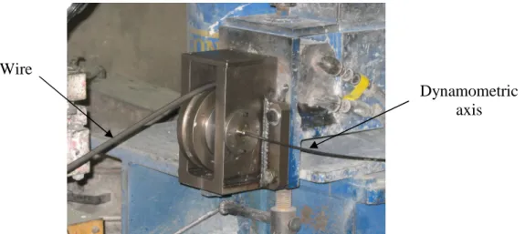
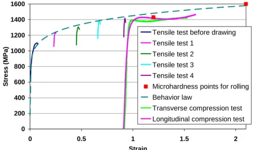
Tout d’abord, l’acier haut carbone a été caractérisé expérimentalement par une large campagne d’essais : essais de traction, compression, torsion, cisaillement tout au long de la gamme de mise en forme à froid. Par ailleurs, les essais de compression ont mis en évidence une ovalisation dans le sens transverse des éprouvettes au cours et en fin de tréfilage qui est la traduction d’une anisotropie mécanique évolutive. C’est pourquoi un critère anisotrope de type Hill quadratique a été choisi pour simuler le comportement du matériau et ses paramètres ont été identifiés à partir de l’équation de contour des éprouvettes de compression. De plus, les paramètres de frottement en tréfilage et en laminage ont été calés, par la mesure de la force de tréfilage avec un axe dynamométrique dans un cas et par des essais de bi poinçonnement dans l’autre cas. Enfin, les paramètres du critère d’endommagement de Lemaître ont été identifiés avant tréfilage afin de pouvoir prédire l’évolution de l’endommagement au cours de la mise en forme.

Ensuite, une fois cette caractérisation effectuée, la simulation du tréfilage et du laminage a été réalisée au moyen d’un logiciel d’éléments finis, FORGE2005®. Une modélisation avec un comportement isotrope a permis d’enrichir les connaissances de ces deux procédés en terme de déformation, taux de déformation, contraintes, prédiction de la géométrie finale… Plusieurs études de sensibilité ont été conduites afin d’apporter des informations supplémentaires. Elles ont concerné le transfèrt des contraintes résiduelles du tréfilage au laminage, l’influence du transport de la cartographie exacte des déformations du tréfilage au laminage. Un résultat majeur de la modélisation isotrope a été la sous estimation de 10% de la largeur du plat en fin de laminage. Enfin, le laminage a été simulé avec une loi de comportement anisotrope, précédemment identifiée. Cette simulation a mis en évidence un fort impact de l’anisotropie mécanique dans la prédiction de l’élargissement des plats puisque que la sous estimation est alors de 5%. Deux études : une sur le frottement et une sur les paramètres de Hill, n’ont pu expliquer ce sous élargissement restant.

Ensuite, une étude microstructurale couplée à une analyse des mécanismes d’endommagement a été effectuée sur les aciers perlitiques à haut carbone au cours du tréfilage et du laminage. L’anisotropie mécanique est issue de l’orientation progressive des colonies perlitiques au tréfilage et de l’apparition d’une texture cristallographique préférentielle. Cette étude a aussi mis en évidence la nature anisotrope de l’endommagement en relation avec l’évolution microstructurale. Trois mécanismes d’endommagement ont pu être identifiés au cours du tréfilage : l’amorçage de cavités au voisinage d’une inclusion dont les mécanismes diffèrent en fonction du type d’inclusion ; l’amorçage de cavités comme une conséquence de rupture transverse des colonies perlitiques défavorablement alignés par rapport à l’axe de tréfilage ; la nucléation de cavités aux joints de colonies fortement désorientées. Au cours du laminage, l’anisotropie mécanique est stoppée. Ce procédé qui se caractérise par une hétérogénéité de déformation entraîne une microstructure différente entre le cœur et les bords du plat, alors que le tréfilage est un procédé de traction avec des déformations homogènes dues à la symétrie de révolution. Cette déformation hétérogène affecte fortement l’évolution de l’endommagement, notamment avec une densité de cavités plus importante à cœur qui est la zone la plus déformée. Le facteur de forme des cavités est aussi fortement lié à cette hétérogénéité. Les décohésions et les cavités qui se développaient selon l’axe de fil au cours du tréfilage sont élargies dans la direction transverse pendant le laminage. Au voisinage des inclusions, les cinétiques de propagation / transport des décohésions sont également modifiées.

L’utilisation de l’outil numérique à apporté des informations supplémentaires. L’évolution morphologique des cavités a été numériquement vérifiée ; elle est en un bon accord avec le champ de déformation. De plus, l’utilisation d’un critère d’endommagement a permis de vérifier la localisation de l’endommagement à cœur, ainsi que d’exhiber un endommagement surfacique pas forcément visible d’un point de vue microstructural et de correctement prédire le risque de rupture.

Enfin, des calculs d’optimisation ont été effectués. Une stratégie d’évolution assistée par méta modèle a été adoptée. Cette méthode a déjà démontré sa robustesse et son efficacité pour des applications complexes de mise en forme. Cette stratégie consiste en une approximation de la simulation numérique afin d’estimer la réponse de la fonction coût. Seules les meilleures solutions probables sont effectivement simulées ce qui permet d’économiser 80% du temps de calcul. L’optimisation du tréfilage à porté sur la géométrie des filières : le demi angle d’entrée de filière, la longueur de portée et la réduction avec des optimisations mono et multi objectifs : la force de tréfilage et l’endommagement. Les calculs ont montré que quelle que soit la fonction coût, la longueur de portée a une influence mineure sur l’optimum par rapport au demi-angle de filière. Par ailleurs, la minimisation de la force de tréfilage a permis de retrouver la notion d’angle optimal, mise en évidence expérimentalement il y a plusieurs

décennies. Par contre, la minimisation de l’endommagement donne un optimum totalement différent avec un angle minimal qui se cale donc sur la borne inférieure. Enfin, l’optimisation mono objectif pondéré des deux fonctions coûts et l’optimisation multi objectif a mis en évidence la possibilité de diminuer fortement l’endommagement sans trop augmenter la force de tréfilage et le risque de rupture.

Table of Content

Chapter I Introduction ____________________________________________________ 10

I.1 Industrial Context ______________________________________________________ 10 I.2 High carbon steel forming processes _______________________________________ 10 I.2.1 Four-stepped wire drawing _____________________________________________________ 12 I.2.2 Cold rolling _________________________________________________________________ 13 I.2.3 Results _____________________________________________________________________ 14 I.2.3.1 Process understanding by means of the triaxiality evolution_______________________ 14 I.2.3.2 Damage prediction_______________________________________________________ 15 I.2.3.3 Final geometry and widening prediction ______________________________________ 17 I.3 Objectives of the thesis __________________________________________________ 19 I.4 Organisation of the thesis ________________________________________________ 19

Chapter II Bibliography Review____________________________________________ 22

II.1 Lamellar microstructure _________________________________________________ 23 II.1.1 Influence of patenting on microstructure and mechanical properties _____________________ 23 II.1.2 Micro - Mesoscopic scale ______________________________________________________ 24 II.1.2.1 Drawn wire ____________________________________________________________ 24 II.1.2.2 Cold rolled sheets _______________________________________________________ 26 II.1.3 Macroscopic scale ____________________________________________________________ 28 II.1.3.1 Drawn wire ____________________________________________________________ 28 II.1.3.2 Cold rolled sheet ________________________________________________________ 28 II.1.4 Summary ___________________________________________________________________ 29 II.2 Yield functions _________________________________________________________ 29 II.2.1 Isotropic yield functions _______________________________________________________ 30 II.2.1.1 Tresca criterion _________________________________________________________ 30 II.2.1.2 Von Mises criterion ______________________________________________________ 30 II.2.1.3 General quadratic and non-quadratic isotropic criterion __________________________ 31 II.2.2 Anisotropic yield functions _____________________________________________________ 33 II.2.2.1 Hill quadratic criterion____________________________________________________ 33 II.2.2.2 Hill non quadratic criterion ________________________________________________ 33 II.2.2.3 Hosford non quadratic criterion _____________________________________________ 33 II.2.2.4 Other anisotropic functions ________________________________________________ 34 II.2.3 Choice of a yield function ______________________________________________________ 35 II.3 Damage mechanisms and models __________________________________________ 36 II.3.1 Ductile damage ______________________________________________________________ 36 II.3.1.1 Ductile damage characterization ____________________________________________ 36 II.3.1.2 Ductile damage mechanisms _______________________________________________ 36 II.3.1.2.1 Nucleation___________________________________________________________ 37 II.3.1.2.2 Growth _____________________________________________________________ 38 II.3.1.2.3 Coalescence _________________________________________________________ 38 II.3.2 Ductile damage models ________________________________________________________ 39 II.3.2.1 Introduction ____________________________________________________________ 39 II.3.2.2 Non-coupled damage models_______________________________________________ 40 II.3.2.2.1 Models based on a microscopic analysis ___________________________________ 40 II.3.2.2.2 Models based on a macroscopic analysis ___________________________________ 43 II.3.2.3 Coupled damage models __________________________________________________ 43 II.3.2.3.1 Damage variable and effective stress concept _______________________________ 44 II.3.2.3.2 Isotropic Lemaître’s model ______________________________________________ 45 II.3.2.3.2.1 General framework of thermodynamics of damage _______________________ 45 II.3.2.3.2.2 State potential for isotropic damage ___________________________________ 46 II.3.2.3.2.3 Formulation of the isotropic unified damage law _________________________ 47

II.3.2.3.2.4 Uniaxial behaviour ________________________________________________ 48 II.3.2.3.3 Tension / compression damage asymmetry, crack closure effects and cut-off value of

stress triaxiality ______________________________________________________ 49 II.3.2.3.4 Framework of porous media plasticity _____________________________________ 50 II.3.2.4 Microscopic numerical modelling ___________________________________________ 50 II.3.2.5 Microscopic experimental modelling ________________________________________ 51 II.3.3 Choice of a relevant damage model ______________________________________________ 52 II.4 Summary______________________________________________________________ 54 II.5 Résumé français ________________________________________________________ 56

Chapter III Experimental mechanical characterisation _________________________ 58

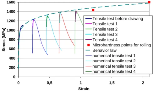
III.1 Identification of a numerical behaviour law _________________________________ 58 III.1.1 Experimental tests _________________________________________________________ 58 III.1.2 Identification method _______________________________________________________ 59 III.2 Identification of friction parameters _______________________________________ 61 III.2.1 Identification of the friction parameter during wire drawing _________________________ 61 III.2.2 Identification of the friction parameter during rolling ______________________________ 62 III.3 Highlighting the anisotropy phenomenon ___________________________________ 63 III.3.1 Compression tests during wire drawing _________________________________________ 63 III.3.1.1 Longitudinal compression tests _____________________________________________ 63 III.3.1.2 Transverse compression tests_______________________________________________ 64 III.3.2 Comparison of the stress-strain curves __________________________________________ 65 III.4 Further mechanical tests _________________________________________________ 66 III.4.1 Torsion test _______________________________________________________________ 66 III.4.1.1 Advantages ____________________________________________________________ 66 III.4.1.2 Results ________________________________________________________________ 67 III.4.1.3 Fields and Backofen method for the stress-strain curve __________________________ 68 III.4.2 Ultimate drawing __________________________________________________________ 68 III.4.3 Complete mechanical behaviour ______________________________________________ 70 III.5 Identification of Hill’s parameters _________________________________________ 71 III.5.1 Anisotropic constitutive model________________________________________________ 71 III.5.2 Coefficients measurement ___________________________________________________ 72 III.5.2.1 At the end of drawing ____________________________________________________ 72 III.5.2.2 At the end of rolling______________________________________________________ 74 III.6 Identification of Lemaître’s parameters ____________________________________ 77 III.6.1 Inverse analysis method _____________________________________________________ 77 III.6.2 Hardening law identification _________________________________________________ 78 III.6.3 Damage parameters identification _____________________________________________ 80 III.7 Summary______________________________________________________________ 82 III.8 Résumé français ________________________________________________________ 83

Chapter IV Process Modelling _____________________________________________ 84

IV.1 The mechanical problem _________________________________________________ 84 IV.1.1 Continuous problem formulation ______________________________________________ 84 IV.1.1.1 Conservation equations ___________________________________________________ 84 IV.1.1.2 Boundary conditions _____________________________________________________ 85 IV.1.1.3 Strong formulation of the continuous problem _________________________________ 86 IV.1.1.4 Weak formulation of the continuous problem __________________________________ 86 IV.1.2 Discretized problem formulation ______________________________________________ 87 IV.1.2.1 Time discretization ______________________________________________________ 87 IV.1.2.2 Spatial discretization _____________________________________________________ 88

IV.2 Cold forming processes simulation_________________________________________ 90 IV.2.1 Isotropic behaviour_________________________________________________________ 91 IV.2.1.1 Strain rate and strain evolution _____________________________________________ 91 IV.2.1.2 Stress evolution during wire drawing ________________________________________ 93 IV.2.1.2.1 Equivalent stress (according to Von Mises) _________________________________ 93 IV.2.1.2.2 RR radial stress evolution ______________________________________________ 93

IV.2.1.2.3 orthoradial stress evolution ___________________________________________ 94

IV.2.1.2.4 xx longitudinal stress evolution __________________________________________ 95

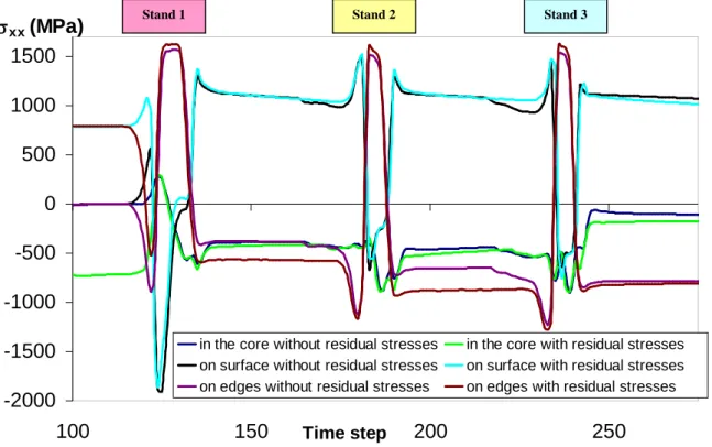
IV.2.1.2.5 xx residual longitudinal stress evolution ___________________________________ 96

IV.2.1.3 Stress evolution during rolling______________________________________________ 97 IV.2.1.3.1 Equivalent stress (according to Von Mises) _________________________________ 97 IV.2.1.3.2 Longitudinal stress ____________________________________________________ 97 IV.2.1.3.3 Transverse stress______________________________________________________ 99 IV.2.1.3.4 Vertical stress ________________________________________________________ 99 IV.2.1.3.5 Danger zones _______________________________________________________ 100 IV.2.1.4 Widening prediction ____________________________________________________ 100 IV.2.2 Sensitivity studies_________________________________________________________ 101 IV.2.2.1 Influence of strain map transfer from drawing to rolling_________________________ 101 IV.2.2.2 Influence of residual stresses transfer from drawing to rolling ____________________ 102 IV.2.3 Influence of anisotropy_____________________________________________________ 104 IV.2.3.1 On strain – stress evolution _______________________________________________ 104 IV.2.3.2 On widening prediction __________________________________________________ 105 IV.2.3.2.1 Sensitivity study on anisotropic coefficients _______________________________ 105 IV.2.3.2.2 Sensitivity study on friction ____________________________________________ 106 IV.3 Conclusions___________________________________________________________ 107 IV.4 Summary_____________________________________________________________ 108 IV.5 Résumé français _______________________________________________________ 109

Chapter V Microstructure and Damage ____________________________________ 110

V.1 Experimental procedure and devices ______________________________________ 110 V.1.1 Experimental devices for micro and nanoscopic analysis _____________________________ 110 V.1.2 Experimental procedure of sample preparation_____________________________________ 111 V.1.2.1 For SEM pictures_______________________________________________________ 111 V.1.2.2 For TEM pictures_______________________________________________________ 111 V.2 Analysis of the first damage steps during ultimate drawing ___________________ 112 V.2.1 Ultimate drawing characteristics ________________________________________________ 112 V.2.2 Microstructural evolution during ultimate drawing: pearlite orientation _________________ 113 V.2.2.1 Before drawing ________________________________________________________ 113 V.2.2.2 After 4 passes (equivalent to the end of drawing in the real process): =0.77_________ 114 V.2.2.3 After 10 passes: =2.1 ___________________________________________________ 115 V.2.2.4 After 16 passes: =3.4 ___________________________________________________ 116 V.2.3 Damage initiation and growth during ultimate drawing ______________________________ 118 V.2.3.1 After 4 passes (equivalent to the end of drawing in the real process): =0.77_________ 118 V.2.3.2 After 10 passes: =2.1 ___________________________________________________ 119 V.2.3.3 After 16 passes: =3.4 ___________________________________________________ 121 V.2.3.4 Synthesis _____________________________________________________________ 122 V.3 Analysis of damage evolution during wire drawing + rolling __________________ 123 V.3.1 Process characteristics________________________________________________________ 123 V.3.2 Microstructural evolution during rolling __________________________________________ 123 V.3.3 Damage evolution during rolling _______________________________________________ 125 V.3.3.1 Transverse cutting plane _________________________________________________ 125 V.3.3.2 Longitudinal cutting plane ________________________________________________ 128 V.4 Schematic representation of damage at the end of rolling _____________________ 130 V.4.1 From experimental observations ________________________________________________ 130 V.4.2 From process numerical simulation by using spherical markers________________________ 132

V.4.3 Comparison between the two representations ______________________________________ 135 V.5 Damage prediction with finite element modelling____________________________ 137 V.6 Summary_____________________________________________________________ 139 V.7 Résumé français _______________________________________________________ 142

Chapter VI Optimization _________________________________________________ 145

VI.1 Optimization strategy __________________________________________________ 145 VI.1.1 Modelling _______________________________________________________________ 145 VI.1.1.1 Choice of the optimization situation / reference configuration ____________________ 146 VI.1.1.2 Choice of optimization parameters and their mathematical translations _____________ 146 VI.1.1.3 Choice of objective functions and constraints and their mathematical translations_____ 147 VI.1.1.4 Definition of parameters limits ____________________________________________ 147 VI.1.2 Selection ________________________________________________________________ 148 VI.1.3 Resolution_______________________________________________________________ 148 VI.2 Optimization methods and their applications to metal forming processes________ 148 VI.2.1 Gradient-based algorithms __________________________________________________ 148 VI.2.2 Global algorithms _________________________________________________________ 149 VI.2.3 Approximate algorithms ____________________________________________________ 151 VI.2.4 Hybrid algorithms_________________________________________________________ 153 VI.3 Choice of an optimization algorithm ______________________________________ 153 VI.3.1 MAES algorithm _________________________________________________________ 154 VI.3.2 Parallel calculations _______________________________________________________ 155 VI.4 Wire drawing optimization ______________________________________________ 155 VI.4.1 Use of the optimization strategy (see VI.1) _____________________________________ 155 VI.4.1.1 Choice of the optimization case____________________________________________ 155 VI.4.1.2 Choice of optimization parameters and their mathematical translations _____________ 156 VI.4.1.3 Choice of objective function and its mathematical translation ____________________ 156 VI.4.1.4 Definition of parameters variation range _____________________________________ 157 VI.4.2 Parameters sensitivity study: optimization of a single drawing pass __________________ 157 VI.4.2.1 Mono-objective optimization______________________________________________ 157 VI.4.2.1.1 Optimization of the drawing force _______________________________________ 157 VI.4.2.1.2 Optimization of damage _______________________________________________ 162 VI.4.2.1.3 Optimization of damage and force _______________________________________ 166 VI.4.2.2 Multi-objective optimization ______________________________________________ 167 VI.4.3 Full wire drawing optimization ______________________________________________ 168 VI.4.4 Toward more objectives ____________________________________________________ 170 VI.5 Summary_____________________________________________________________ 171 VI.6 Résumé français _______________________________________________________ 172

Chapter VII Conclusions and Perspectives _________________________________ 174 ANNEXES ______________________________________________________________ 177

ANNEX 1: Framework of porous media plasticity _________________________________ 177 ANNEX 2: Anisotropic damage models __________________________________________ 179 ANNEX 3: Fields and Backofen method for the stress-strain curves __________________ 183 ANNEX 4: Explicative notice of a Focused Ion Beam (FIB)__________________________ 187

Chapter I Introduction

I.1

Industrial Context

ArcelorMittal produces flat and shape wires with quite a few different steel grades. For instance, flat-rolled steel wires are used in automotive industries and thus they have to be accurate in terms of final geometry and mechanical properties. Furthermore, flawlessness is a major point of technical specifications in order to avoid break risks in use or during production. Since ever-higher mechanical characteristics and more complex geometries are required, the limits of the current forming processes tend to be reached. Consequently, damage prediction appears as a major point in order to avoid material fracture.

The different damage steps: nucleation, growth and coalescence during forming processes need to be better understood in the case of the high carbon steels involved in this study. Experiments as well as numerical simulation will be used for this purpose. Thanks to this, process optimization will be carried out with adequate algorithms for high strain processes.

I.2

High carbon steel forming processes

The overall manufacturing process involves seven major steps from continuous casting to final heat treatment as shown in Figure 1. The present work focuses on the two cold processes which are wire drawing on single-pass benches followed by multi-pass tandem rolling (Figure 2), starting from a patented wire rod. Patenting is a thermal treatment in which the hot-rolled wire is:

 Heated to a temperature higher than the austenitizing temperature (about 900°C)

 Cooled down in a lead bath (> 500°C) during a given time.

This results in a very fine wire microstructure (fine pearlite) and in excellent trade-off between high strength and high ductility.

Continuous casting

Hot rolling Heat treatments Wire drawing Cold rolling

Final Heat treatment

Patenting

Figure 2: The cold forming processes

The material is a high carbon steel grade C72, i.e. the weight percentage of carbon is near the eutectoid point in the Iron-Iron Carbide phase diagram as shown in Figure 3.

Figure 3: Fe-Fe3C Phase Diagram [1]

The microstructure is then pearlitic: ferrite with lamellar cementite. SEM pictures show cementite lamellae in white and ferrite in dark (Figure 4). The microstructure is homogeneous. Grains are equiaxed, with a random crystallographic texture. As there is a crystallographic orientation relationship between ferrite and cementite [2], lamellae have the

same orientation within a grain, but the random grain texture gives overall random lamellae and ferrite orientation.

Figure 4: Initial high carbon steel microstructure (patented wire) [3]

Following [4] and [5], the industrial drawing and flat-rolling process has been simulated by FEM (Forge2005®). This first attempt at numerical modelling will show some discrepancies with experiments, the correction of which will be addressed in the following chapters.

I.2.1 Four-stepped wire drawing

This forming process consists in reducing product section by pulling the wire through a single or series of drawing dies [6] (Figure 2). To make this operation easier, it needs lubrication at the entrance. This is done by a soap box situated upstream of each drawing die. A high strength level is reached by hardening and will be increased by rolling.

The mechanical analysis of the drawing process is performed with FORGE2005® on a 2D axis-symmetric simulation (rθ = 0) (Figure 5). The patented wire rod is isotropic before

drawing. All properties acquired during each step are transferred to the next one in order to take into account progressive material hardening. Mesh size is equal to 0.5mm and the total nodes number is about 9600 for pass one and two and about 11500 and 12700 nodes for pass

three and four respectively. The wire is long enough to reach the steady state. A non deformable die is used to set drawing speed.

Figure 5 : Beginning of the wire drawing simulation

An elasto-plastic behaviour law is used [5] and will be detailed in section III.1:

) 32 . 7 1 ( 64 . 100 * 3 0.13    (I.1)

Friction law between drawing dies and wire is a Tresca law: 02 . 0 3 _ 0 _  m with m c





The identification of the friction coefficient will be presented in section III.2.1. At the end of drawing, strain and stress values are transferred to rolling simulation.

I.2.2 Cold rolling

This is a forming process by plastic deformation (Figure 2), bound to decrease product section thanks to two axisymmetric tools called “cylinders” [7]. Wire is pulled in the roll gap by their rotation. This operation imparts the wire with both the required final geometry and mechanical strength. The rolling mill has three stands which work in tandem, which means the wire is in the three stands simultaneously. Each stand is simulated separately in order to introduce proper interstand tension, which have been measured on the rolling line.

The process geometry calls for a 3D modelling but two symmetry planes are used to reduce computing time (Figure 6). The same workhardening equation is used and the same friction law but with 0.25

_



m due to a different lubricant (low concentration oil in water emulsion). The identification of the friction coefficient will be introduced in part III.2.2. During 2D – 3D transfer, a manual remeshing took place and mesh size before rolling is 0.5mm leading to a total nodes number of 22000. At the beginning of the simulation a pushing die helps gripping of the wire by the cylinder, and then the cylinders become masters.

Figure 6: Beginning of the rolling simulation

I.2.3 Results

I.2.3.1 Process understanding by means of the triaxiality evolution

Triaxiality is the ratio between the hydrostatic pressure and the equivalent stress.

Figure 7: Triaxiality evolution during wire drawing

Pass 1 Pass 2 Pass 3 Pass 4 1 0 -1.5 x y z

A triaxiality analysis enables to understand the mechanical behaviour during forming and is presented in Figure 7 and Figure 8. Wire drawing process is mainly compressive in the wire core with local tensile areas. During rolling, the triaxiality is mainly compressive as well in the wire core but also tensile on edges.

Figure 8: Triaxiality evolution during rolling

I.2.3.2 Damage prediction

A first analysis of damage has been done with the use of a macroscopic non coupled criterion, i.e. Latham and Cockcroft criterion which is written as follows:

1 0 -1.5 Stand 1 Stand 2 Stand 3 x y z



These criteria determine a critical value, constant at fracture and supposed independent on strain path. Damage evolution during wire drawing followed by rolling exhibits in the wire core a severe and constant increase at each pass of drawing and at the first rolling stand, as shown in Figure 9, Figure 10 and Figure 11.

0 0,1 0,2 0,3 0,4 0,5 0,6 0,7 0,8 Time Da m a g e latham et Cockcroft

Stand 1 Stand 2 Stand 3

pass 2 pass 3 pass 4 pass 1

WIRE DRAWING

ROLLING

Figure 9: Latham and Cockcroft damage evolution during cold forming processes in the wire core

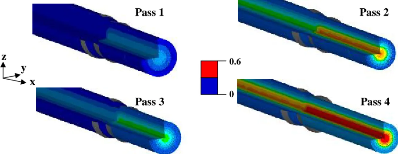
Figure 10: Damage evolution during wire drawing with Latham and Cockcroft's criterion

Pass 1 Pass 2 Pass 3 Pass 4 0.6 0 x y z

Figure 11: Damage evolution during rolling stand with Latham and Cockcroft's criterion

I.2.3.3 Final geometry and widening prediction

As mentioned before, a major point to monitor is the output geometry after cold forming processes, as it is a critical aspect of technical specifications. However, when comparing the experimental and computed final cross-sections, a difference appears: the computed section is too narrow by  10%, way above the tolerance (Figure 12).

Computed cross-section with

isotropic bulk model FORGE2005

Figure 12: Comparison of experimental and computed (dark red line) output cross-sections

This difference might originate in the anisotropy introduced by the wire drawing process, coming either from a crystallographic or a morphological texture (grain elongation). In the case of high carbon steels, another probable origin of mechanical anisotropy is the progressive

Stand 1 Stand 2

Stand 3 x

y z

cementite interlamellar spacing (Figure 13, Figure 4 and Figure 14) [8]-[12]. The structure alignment is a major contribution to the development of a strong crystallographic texture [13]-[16]. All this explains the appearance and evolution of a strong anisotropy, as well as changes in the mechanical properties [17], [18]. This mechanical anisotropy may have a non-negligible influence on damage mechanisms as well.

Figure 13: Evolution of the interlamellar spacing (a) before drawing (b) after drawing [3]

Figure 14: High carbon steel microstructure after drawing [3]

2 µm

2 µm 2 µm2 µm

Wire drawing axis

(a)

(b)

Wire drawing axis Bent lamellae during drawing

I.3

Objectives of the thesis

This thesis aims at better understanding cold forming processes for high carbon steel in order to propose a semi-automatic multi-criteria process optimization. Before using FEM simulation to optimize both processes, we have to guarantee good control of adequate numerical options and a proper material behaviour (damage and plasticity laws), with geometry (width) and damage as quality criteria.

Mechanical behaviour will be studied thanks to an experimental campaign, as well as friction coefficient between dies and the wire. Then, mechanical analysis will be performed by simulating the two processes, with the material behaviour law previously identified from mechanical tests, in Forge2005®.

Concerning damage mechanisms, the same approach will be used, i.e. a microstructural analysis of damage will be carried out to better understand damage mechanisms; then an adapted damage function will be used in the finite element code to predict damage and fracture risks.

Then the road will be open for the last major issue, semi-automatic process optimization. The objective function will be built on the major requirements for a given product (either final mechanical properties, or geometry, or damage risk, or any multi-objective combination of these). Ideally, optimization parameters may refer to the preform (wire rod diameter), to the drawing process (number of passes, total reduction), and / or to the rolling process (number of passes, reductions, roll shape). But accounting for all requirements and all optimization parameters simultaneously would be far too complex. Part of the work will consist in designing simplified approaches of relevant sub-problems, based on our knowledge of the processes and material evolution.

I.4

Organisation of the thesis

This PhD report is organised as follows.

The following chapter (Chapter II) will introduce a bibliographical review useful to understand the whole of results that I will discuss. High carbon steel microstructure, mechanical behaviour, forming … will be addressed first. In a second part, a review will be given on anisotropic behaviour laws to guide the reader toward the chosen anisotropic criterion for our process simulation. Anisotropy is a known phenomenon for sheet rolling but very few articles deal with bulk material; this is one of the innovative points of this thesis. Finally, the last section will be dedicated to damage mechanisms and ductile damage models. Both isotropic (to introduce major damage theory) and anisotropic damage models will be

implementation of each function in order to give some clues as to the relevant damage model adapted to the two cold forming processes.

High carbon steel is used for this study and a complete understanding of its behaviour is required. Hence, experimental measurements will be described in Chapter III, presenting mechanical testing devices for tension, compression, shear and torsion tests. Experimental results will lead to the identification of a numerical behaviour law and to the confirmation of the existence of a strong mechanical anisotropy. Procedure adjustment for numerical parameters identification, i.e. anisotropic coefficients, will also be raised in this part, as well as the identification of damage parameters. Additional tests will be carried out to fit friction parameter.

The first results will concern a complete modelling of wire drawing and rolling processes and will be discussed in Chapter IV. Stress and strain state during cold forming process will be described in depth, insisting on strain heterogeneity. Furthermore, emphasis will be on the width prediction, i.e. comparison between experimental and simulated output cross-sections and thus, to see if the introduction of anisotropic behaviour law in our simulation improve and lead to a correct widening estimation. Finally these numerical results will be complemented with parametric studies on friction, interstand tension and on the influence of transferring or not wire drawing residual stresses from drawing to rolling.

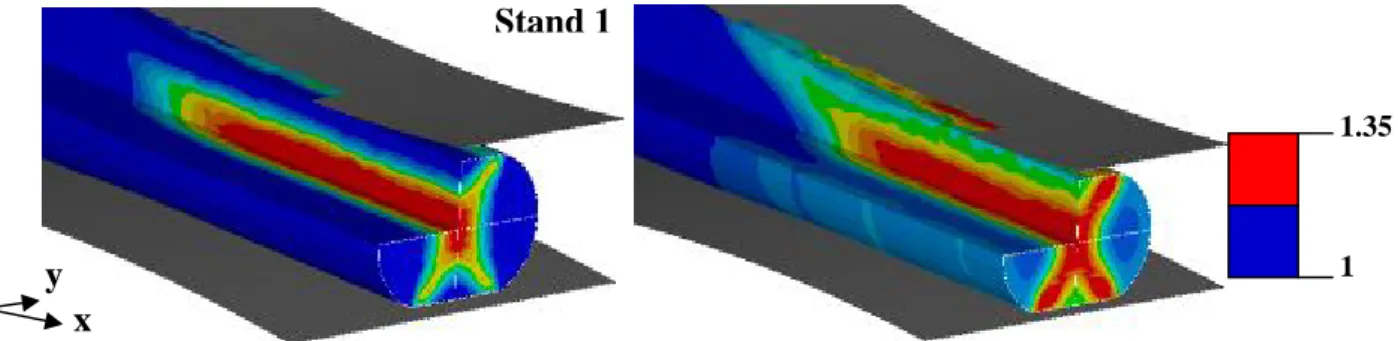
Chapter V will focus on microstructure and damage. In a first step, a detailed experimental study of our two processes will be described. An ultimate wire drawing test procedure (different from the classical wire drawing industrial process) has been run to follow microstructural evolution and explain the appearance of an evolutive anisotropy to extreme limits in deformation. This extreme drawing will lead to the understanding of initiation and propagation damage stages during wire drawing, strongly linked to the anisotropic material flow, thanks to diverse microscopy techniques (optical microscopy [OM], Scanning Electron Microscopy [SEM], Focused Ion Beam / Transmission Electron Microscopy [FIB/TEM]). Then, the microstructural and damage evolution during rolling will be studied. As wire drawing and rolling have different strain paths, due to different process mechanics (wire drawing = axisymmetric section reduction with longitudinal elongation; rolling = vertical compression with transverse and longitudinal elongation), microstructure evolution will be modified as well as damage kinetics. It will be shown that strain heterogeneity during rolling has a deep impact on these two characteristics. A second step will bring new elements for the understanding of damage kinetics by the use of simulation. Virtual spherical markers will be used along forming simulation. Following their morphology as a function of their position in the wire give a very visual understanding of strain components heterogeneity in 3D. Finally,

analysis of a damage criterion will give further insight when comparing experimental and numerical damage maps during the process.

Optimization will be addressed in Chapter VI, starting with a bibliographical review of optimization methods, which are part of a wider optimization strategy. The choice of a MAES strategy (Meta-model Assisted Evolution Strategy) proposed by Emmerich and al. [19], will be justified. Then a second part will be about wire drawing optimization. Objective function, i.e. damage criterion, and optimization parameters will be introduced. A study on a single pass will be presented, focussing on the following points: drawing force as objective function, damage as objective function, influence of reduction and friction, simultaneous minimization of drawing force and damage, study of “skin-pass” (low reduction drawing). Finally, I will go on with the optimization of a four-stepped wire drawing sequence.

Overall results of this work will be summarized in the conclusions and perspectives chapter (Chapter VII), in terms of modelling and anisotropy, microstructure and damage. Directions will be given for further improvements of this study.

Chapter II Bibliography Review

Steels are widely used in forming. Depending on applications, steels are used in different grades. The higher the carbon content of the steel is, the higher the initial strength is, for a given structure [6]. Thus, low carbon steels are used for staple, paper clip, screw and so on, whereas high carbon steels are used for heavy-duty pieces, e.g. for high strength wire like tire frames. Wires are joined together to make heavy-duty cables.

The carbon content determines the steel microstructure as it is shown in the Fe-Fe3C phase

diagram (Figure 3); it therefore impacts on mechanical properties. For four decades, microstructure and mechanical properties evolution during forming processes have been investigated by a large scientific community. This has been done e.g. to understand the origin of fracture during wire drawing, which is strongly linked to the microstructure evolution. Then several authors tried to model the microstructure evolution at different scales. The first section presents the assessment of these researches for high carbon steels. Then investigation field is broadened with other lamellar alloys.

The main result of the primary simulation presented in chapter 1 will lead us to study the anisotropic behaviour of our high carbon steel, introduced by the wire drawing process. Plastic anisotropy is defined by different flow properties (tensile yield stress e.g.) in the three spatial directions. This difference in yield stress favours flow in one cross-sectional direction with respect to the other; an experimental manifestation is the ovalization of tensile or compression samples. Thus, anisotropy may be analysed both using stress and strain rate tensors. Since the 50’s, many authors have tried to model anisotropy by different ways in order to predict both phenomena simultaneously. But fitting ovalization and yield stress is difficult. This difficulty is usual in sheet forming, where it is very hard to fit the angular dependence of both flow pattern (Lankford coefficient [20]) and yield stress. Thus, paragraph II.2 is devoted to a brief summary of the different kinds of anisotropic laws from the simplest to the more complex representation.

Damage mechanisms on steels have been extensively described and understood since several decades. A lot of criteria and damage laws have been developed in order to make good and accurate prediction of this physical phenomenon. Section II.3 aims at reminding the three steps of ductile damage mechanisms and at making the state of art of damage models.

II.1 Lamellar microstructure

After the first two processes which are continuous casting and hot rolling followed by some heat treatments, steel is ready to be cold drawn and cold rolled to reach a high strength and a given geometry. To improve ductility and strength in the two cold processes, patenting (austenitization followed by quenching in a lead bath) is performed before cold forming.

II.1.1 Influence of patenting on microstructure and mechanical properties

Patenting consists in heating the wire in a furnace above the austenitizing temperature (900-1000°C). This high temperature treatment produces uniform austenite of rather large grain size. The subsequent quench of small sections (e.g. wire rods) in molten lead – at a temperature higher than 500°C - gives very fine pearlite, preferably with no separation of primary ferrite [21]. Microstructure after patenting is shown in Figure 15.

Figure 15: Pearlite in a patented steel wire; an insert shows pearlite colonies [15]

In terms of mechanical properties, patenting leads to an increase of the strength and the ductility as shown in Table 1. (NB: Agt means elongation).

Grade

Step Rp0,2 (MPa) Rm (MPa) Agt% A % Z %

C72

Blank

539

978

9.0 14.8 34.8

Now, this microstructure can undergo different physical phenomena in function of forming processes. We are going to detail these phenomena with the observation scale as classification.

II.1.2 Micro - Mesoscopic scale

II.1.2.1 Drawn wire

To study the microstructure evolution and deformation mechanisms, the best example is ultimate drawing (the wire is drawn until mechanical limit is reached) where very high strain is obtained. Steel cord is processed using this technique, and it is very interesting from a scientific point of view.

At a mesoscopic level, it produces changes in pearlite colonies. Both, longitudinal and cross-sections are studied to have a 3D representation of microstructure evolution, which is controlled by different mechanisms in each direction. In a longitudinal view, the effect of drawing on microstructure is a progressive orientation of pearlite colonies by alignment of cementite lamellae (Figure 16) with its main axis approaching the wire axis [11], [12]. A relation can be obtained between drawing strain and the orientation of a colony characterized by an angle  with regard to the wire axis [15]; its dependence on the initial angle  is

illustrated in Figure 17.

Furthermore, wire drawing causes a decrease of interlamellar spacing [8]-[12], [15], [22] as illustrated in Figure 18. Lamellae also become thinner. When the lamellar spacing of pearlite is decreasing, hardening of the drawn pearlitic steels is observed [18] and steel is more ductile. This can be explained by the thin cementite lamellae of fine pearlite being able to undergo substantial deformation by bending [23].

Figure 16: SEM longitudinal micrographs showing microstructural changes with drawing strain for an eutectoid steel – (a)  = 0, (b)  = 0.91, (c)  = 2.32 [11]

Figure 17: Dependence of α-angle as a function of

drawing strain [15] Figure 18: Inter-lamellar spacing as a function of drawing strain [15]

When samples are cut in the transverse direction, micrographs show the familiar swirled microstructure (Figure 19) due to a radial orientation of [001] direction of ferrite [15].

Figure 19: TEM pictures of transverse section of drawn wires of axially oriented pearlite with true strains of 4.2. [9]

In addition to the radial orientation, a crystallographic texture appears in drawn wires [8], [13]-[16]: a [110]-type texture of ferrite. Work performed on large diameter wires [24] indicates that [110] fibre texture results in an alignment of (001) planes, which are cleavage planes in ferrite.

It is clear that damage will be strongly linked to this microstructural evolution. Many data are available on damage of cold drawn steels but most of them concern the macroscopic delamination phenomenon during torsion tests [25], [26] and is not of interest in this study because it happens at higher drawing strain. On the other hand, wire drawing at high strains presents some other interesting damage mechanisms.

M. Yilmaz [27], in a survey of experimental studies on the causes of ductile fracture of high carbon steel wires since 1994, has highlighted a predominant role of non-metallic inclusions also called ceramic inclusions in a broken drawn wire. Because of their strength level, these inclusions are not deformed but broken. Indeed, in an analysis of 121 fractures,

0

reoxidation is the main cause of occurrence of these inclusions: during the continuous casting process, molten steel which was deoxidized beforehand can reoxidize.

Table 2: failure reasons during wire drawing [27] Figure 20: Failure rate during steel wire production and service [27]

This observation was also made by S. Tandon et al. [28], who explain that these inclusions locally increase the tensile strength, preventing material flow.

Microscopic observations identified three mechanisms during deformation: slip in ferrite in the plane parallel to the lamella plane, slip in ferrite crossing lamellae, and slip in the interphase at interfaces [9], [18]. At high strain, deformation mechanisms cause the bending and rupture of cementite lamellae. Moreover, plastic strain and dislocation structure development occur in the ferrite interlayer as well as in cementite [9], [18]. In a first step, dislocation mobility favours the diffusion of carbon atoms and in a second step, dislocations are stopped by interstitial carbon atoms and blocked at the interface between ferrite and cementite. Dislocation structure depends on the pearlite fineness [18].

At a very low scale, many authors have shown that successive drawing passes are responsible for cementite decomposition [23], [29], [30], “dissolution of cementite lamellae”, i.e. diffusion of the cementite carbon into ferrite [23], [30], [31], leading to a local increase of carbon content in lamellar ferrite [32]-[36].

II.1.2.2 Cold rolled sheets

As mentioned in the introduction, only few researchers have worked on flat and sheet cold rolling in terms of microstructure evolution, whereas wire drawing has been studied in depth. However, some interesting results appear in their studies in case of severe cold rolling (up to ~80%). 1 2 3 4 5 6

Figure 21: Typical SEM microstructure of the 0.76C steel transformed at 823 K and cold rolled by 80 %. (a) Low magnification micrograph and the magnified images of (b) IBL, (c) CLS and (d) FL. (ND =

Normal direction and RD = Rolling Direction [37]

Typical SEM pictures of pearlitic steel after severe cold rolling reveal a non-uniform deformed structure [37], [38]. From the micrograph Figure 21a, three kinds of microstructural elements have been identified, they are shown magnified below: bent lamella (IBL, Figure 21b), shear band (CLS, Figure 21c) and fine lamella (FL, Figure 21d). During deformation, the amount of the three types of microstructure evolves differently. As rolling reduction increases:

 FL increases [37], [38].  IBL decreases [37], [38].

 CLS reaches his highest value at 66.5% and then decreases [38].

Based on the classification of the pearlite structure proposed by Takahashi [39], the two authors [37], [38] agree on the deformation mechanisms leading to the heterogeneous microstructure previously presented:

 IBL is formed by compressing the colony with the lamellar direction nearly perpendicular to the rolling plane.

 CLS is formed when the deformation increases, bent lamella continuously converts into shear bands during cold rolling.

 FL is formed at the beginning of cold rolling in the colony with the lamellar direction nearly parallel to the rolling plane.

II.1.3 Macroscopic scale

II.1.3.1 Drawn wire

Tensile solicitation as in cold drawing is used to increase the yield stress by activating a strain hardening mechanism at a macroscopic scale. We have seen in section II.1.2 that tension results in an anisotropic texture and microstructure. Now, mechanical properties are deeply linked to the microstructure evolution as ductility, hardness, stress, strain…Therefore, it results in anisotropic mechanical properties [15], [40].

For instance, ductility increases with the pearlite refinement [18]. In terms of hardness, it increases if: the interlamellar spacing decreases, the dislocation density increases [23] or other alloying elements are used [40], [41]. The yield stress is much higher in case of pearlitic steel with fine-lamellar structure [18] and some authors have shown the dependency of the yield stress on the interlamellar spacing for a number of pearlitic steels containing 0.6–0.8% carbon [23], [42]: 2 / 1 0 0    _y K_pt y   (II.1)

with t0=tfer + tcem (tfer is the thickness of the ferrite interlayer and tcem the thickness of a

cementite lamella). This is similar to Hall and Petch’s law, but here the grain size is replaced by the interlamellar spacing as the relevant microstructural dimension.

II.1.3.2 Cold rolled sheet

In cold rolling, tensile tests enabled the authors to identify a relationship between the true strain and the macroscopic tensile strength for different steels (Figure 22):

 Tensile strength increases with increasing carbon content.  Tensile strength increases with increasing rolling reduction.

Figure 22: Relationship between true strain in rolling and tensile strength; the 0.6C, 0.76C and 1.0C steels transformed at 823 K and cold rolled

[37]

Figure 23: Relationship between yield strength and true strain [38]

As in wire drawing, the interlamellar spacing controls the yield strength of fully pearlitic steels. Two methods can be used to express the yield strength. If the main goal is to precisely evaluate the yield stress, predictive equations can be used together with the interlamellar distance measurement. Several researchers [9], [43]-[45] have used this approach to calculate the yield strength. The measurement of the interlamellar spacing is very difficult and many precautions must be taken, but it gives access to a local measurement of the stress. It is clear that the inhomogeneous microstructure will lead to heterogeneous mechanical properties. On the contrary, if only an estimation of the space-averaged yield strength is needed, a phenomenological, predictive equation using the true strain is sufficient. It is less precise than using the interlamellar distance but gives good macroscopic results as shown in Figure 23 with Hollomon’s equation which links the yield stress with the plastic strain.

II.1.4 Summary

In this section, we have seen the evolution of lamellar microstructure depending on the solicitation (here, tension as in wire drawing and compression as in rolling), as well as their deformation mechanisms. We have also seen that the microstructural evolution has a deep impact on mechanical properties and damage mechanisms. It appears that flat rolling is less documented in terms of damage evolution and justifies a damage study along cold forming processes for high carbon steel in order to identify a damage law. Moreover, high carbon steels show a strong anisotropy. How could it be taken into account in process simulation? The next section answers that question.

II.2 Yield functions

In order to represent plastic behaviour of steels, a phenomenological (or macroscopic) elasto-plastic approach is commonly used. It is then typical to employ a yield function (to describe the yield surface), associated to the normality rule and to a hardening law. The yield surface, defined in the stress space, corresponds to the elastic limit and the beginning of the plastic flow and is written in the following way:

 

 f

f   _u (II.2)

In this equation, 

 

stress which represents the plastic threshold stress.

strain rate components. The yield function gives the stress at which yielding occurs for a given stress state and its gradient (normality rule) gives the direction of the plastic strain rate:





 is the plastic multiplier. This equation is the associated plastic flow law because the yield surface is taken as the dissipative plastic potentialg. When the plastic potential differs from the yield function, equation II.3 is non-associated and becomes:

0 ,            g p (II.4) The hardening law expresses the evolution of the yield surface during deformation. It can be isotropic or anisotropic (e.g. kinematic) hardening, representing respectively the yield surface homothetic inflation / translation.

The yield function may be either isotropic (Von Mises, Tresca, Hosford 1) or anisotropic (Hill, Hosford 2, Barlat…); it may be associated or not. In this section II.2, a sample of yield functions is introduced. Isotropic yield functions are presented first, as an introduction to better understand anisotropic criteria. Then, the choice of a criterion for the present work will be discussed.

II.2.1 Isotropic yield functions

II.2.1.1 Tresca criterion

The oldest criterion is the criterion of Tresca [55] and is written, in principal axes, by:





It expresses that plastification appears once the highest shear stress, in the Mohr representation, reaches a constant critical value, 0.

II.2.1.2 Von Mises criterion

The most used quadratic criterion is Von Mises’ [56], written in an orthonormal frame as:





In principal axes, eq. II.2 becomes:





The next figure (Figure 24) represents the superposition of the two criteria in generalized plane stresses. This one shows that both criteria coincide under some loadings: intersection

with axes corresponds to simple tension / compression; the first bisector corresponds to equilibrated biaxial tension / compression. However, both criteria disagree in shear loading (second bisector), i.e. the ratio between shear and tensile stress (1/2 vs. 1/√3). Moreover, this figure shows no Bauschinger effect as Re in tension equal Re in compression. Finally, the isotropy is characterized by the symmetry compared to the bisectors (axis 1 = axis 2).

II.2.1.3 General quadratic and non-quadratic isotropic criterion

It has been often observed, in experiments or using self-consistent crystal plasticity models, that real criteria lie between the Von Mises and Tresca criteria. Therefore, Hershey has proposed to capture the conclusions of a self-consistent crystal plasticity model by a generalization of both Von Mises and Tresca criteria of the following form [57]:

_f n n n n 0 2 1 1 3 3 2 ( ) 2 1 ) ( 2 1 ) ( 2 1               (II.8)

Note that this yield function remains isotropic, since all three directions play the same role (circular permutation of principal stresses). When n = 2 it reduces to the Von Mises criterion. Hosford extended this function to a non-quadratic criterion [58] :





He showed that this function is also a good approximation for a full-constraint crystal plasticity model [58], and that the stress exponent is strongly coupled to the polycrystalline structure: the best values for n are 6 for BCC and 8 for FCC materials [59], as shown in Figure 25.

For a more complete review of isotropic formulations, Yu [60] presents a bibliographical article on strength theories since the beginning.

Figure 24 : Comparison between Tresca and Von Mises criteria for generalized plane stresses

Figure 25 : Representative Section of Isotropic Yield Loci with 3= 0. Tresca and von Mises are compared with calculations based on the {111 }<110> slip for fcc and <lll>-pencil glide for bcc. Note the 1/Y scale is expanded relative to the 2/Y scale for ease of comparison. The dash and dotted lines represent eq. 10 with

exponents a=8 suggested for fcc and a=6 for bcc (a corresponds to n in equation II.8 and II.9 [59] 1

II.2.2 Anisotropic yield functions

The previous models are not able to predict correctly, in terms of geometry and plastic properties, the anisotropy introduced by some manufacturing processes such as flat or sheet cold rolling. As a consequence, many authors proposed new or modified criteria.

II.2.2.1 Hill quadratic criterion

The first yield function accounting for orthogonal anisotropy was introduced by Hill [61] and is based on Von Mises work. To introduce anisotropy, Hill kept the Von Mises quadratic form, but added six coefficients to describe the direction-dependent plastic flow properties:





f          (II.10)

II.2.2.2 Hill non quadratic criterion

In 1979, R. Hill generalized his yield criterion under the following form [62]:

m m m m m m m N M L H G F f 0 2 1 3 1 3 2 3 2 1 2 1 1 3 3 2 2 2 2                                (II.11) where

σ

after “anisotropizing” Von Mises’ criterion, Hill “anisotropized” Hosford’s criterion (1972).

II.2.2.3 Hosford non quadratic criterion

In 1979, Hosford [63] generalized his isotropic yield function to take into account normal anisotropy(here for a plane stress situation):

0 1 2 1 2 1 1 ) ( 1 1      _             n n n n R R R f (II.12)

This criterion is also a generalization of Hill’s quadratic function for plane stress [64].

To summarize and compare the three previous yield criteria we can observe the next figure (Figure 26). We note that the initial shape of the yield surface is quite different and the evolution of the plane stress state is not the same when the R-coefficient changes.

Figure 26: Evolution of the plane stress state with the anisotropic coefficient R, for three different yield criteria [65]

II.2.2.4 Other anisotropic functions

From this date, many yield criteria have been proposed to accurately predict the real process, by refining the yield surface description by taking into account more and more experimental results. Reviews on these improvements can be found in Barlat and al. [65] and in Hu [67].

Many authors must be cited, who tried to give accurate anisotropy predictions: Barlat and Lian [68], Karafillis and Boyce [69], Darrieulat and Montheillet [70], Bron and Besson [71], Banabic et al. [72], Cazacu et al. [73]. In their approaches, anisotropy is introduced by means of a linear stress transformation (anisotropic combinations of the stress components, based on linear transformation, are used in yield function). The main advantages is the easy development of convex formulations which lead to numerical simulations stability, as explained in Barlat et al. [74].

In the Figure 27, some yield criteria shapes are compared to show the range of yield function shapes achievable.