Regional trend detection and power analyses for chemical parameters monitored at the CWS LRTAP biomonitoring sites in Algoma, Muskoka and Sudbury (1988-1995).

(1)

Record Number: 11950

Author, Monographic: Cluis, D.//Laberge, C. Author Role:

Title, Monographic: Regional trend detection and power analyses for chemical parameters monitored at the CWS LRTAP biomonitoring sites in Algoma, Muskoka and Sudbury (1988-1995)

Translated Title: Reprint Status: Edition:

Author, Subsidiary: Author Role:

Place of Publication: Québec Publisher Name: INRS-Eau Date of Publication: 1996

Original Publication Date: Mai 1996 Volume Identification:

Extent of Work: iii, 89 Packaging Method: pages Series Editor:

Series Editor Role:

Series Title: INRS-Eau, rapport de recherche Series Volume ID: 445

Location/URL:

ISBN: 2-89146-464-8

Notes: Rapport annuel 1996-1997

Abstract: Contrat # KR405-5-0179 - Environnement Canada CWS, Ontarion region LRTAP program 10.00$

Call Number: R000445

(2)

REGIONAL TREND DETECTION AND POWER ANALYSES AT

ALGOMA, MUSKOKA AND SUDBURY BIOMONITORING SITES (1988-1995)

(3)

REGIONAL TREND DETECTION AND POWER ANALYSES

FOR CHEMICAL PARAMETERS MONITORED AT THE CWS LRTAP BIOMONITORING SITES IN ALGOMA, MUSKOKA AND SUDBURY

(1988-1995) Contract # KR405-5-0179 Environment Canada CWS ,Ontario Region LRTAP Program by

Daniel Cluis and Claude Laberge

INRS-EAU

Report # 445 May 1996

(4)

ABSTRACT

This report presents the first results of regional regressions over time performed on data sets containing chemical analyses of parameters measured for different groupings of lakes of the Muskoka, Aigoma and Sudbury regions. The data analysed were monitored as part of the Canadian Wildlife Service Monitoring Program (LRTAP).

For each region, data are available for 17 parameters. The regional trend detection analyses are performed using simple linear regression. The results in this part of the contract are of two kinds:

• Brief result summary for ail combinations of parameters (17) x regions (3) x classification levels (18) : 918 regressions. The results presented are: number of observations, RMSE, slope, significance of slope, predicted value for 1990 (initial) and for 1995 (final). Given the large number of regressions to be performed, no validation of the results are presented. The absence of validation forces the user to : a) validate the results before using them in particular studies or; b) use the results as descriptives.

• Complete regression analyses for pH, alcalinity, calcium and sulfate values in each of the three regions. The analyses include a graphical exploratory data analysis.

(5)

TABLE OF CONTENTS

Section 1: Regional trend detection analyses ... 1

1.1

Results of regional regressions for ail combinations of regions and classifications ...

1

1.1.1

Results when no classification is used ...

1

1.1.2

Regional regression results associated to levels of classification

#1 ... 2

1.1.3 #2 ... 2

1.1.4 #3 ... 2

1.1.5 #4 ... 2

1.2

Summary for each parameter ... 3

1.2.1

pH values ...

3

1.2.2

Conductivity values ...

3

1.2.3

Alkalinity values ...

4

1.2.4

Calcium concentrations ...

4

1.2.5

Magnesium concentrations ...

4

1.2.6

Potassium concentrations ...

5

1.2.7

Sodium concentrations ... 5

1.2.8

Sulfate concentrations ... 6

1.2.9

Silicate concentrations ...

6

1.2.10

Chloride concentrations ...

6

1.2.11

TIC concentrations ... 7

1.2.12

DOC concentrations ... 7

1.2.13

TKN concentrations ... 7

1.2.14

N02N03 concentrations ... 7

1.2.15

Total nitrogen concentrations ... 7

1.2.16

Ammoniac concentrations ... 8

1.2.17

Total phosphorus concentrations ... 8

Section 2: Complete regression analyses ... 9

2.1

pH values ... 9

2.2

Alkalinity values ...

15

2.3

Calcium concentrations ...

22

2.4

Sulfate concentrations ...

29

Section 3: Considerations for regional trend detection ...

35

3.1

Establishment of a sound population survey design ...

35

3.2

Choice of a regional trend detection method ...

35

3.3

Study of the presence of possible autocorrelation ...

36

3.4

Study of the presence of possible spatial correlation ...

39

(6)

LIST OF FIGURES

Figure 1 : Box-Plot graph for the pH values in the Muskoka region ... 9

Figure 2: Scatterplot of pH values in the Muskoka region with regional regression line ... 10

Figure 3 : Normal probability plot of residuals for pH values in the Muskoka region ... 11

Figure 4 : Box-Plot graph for the pH values in the Aigoma region ... 11

Figure 5: Scatterplot of pH values in the Algoma region with regional regression line ... 12

Figure 6 : Normal probability plot of residuals for pH values in the Algoma region ... 13

Figure 7 : Box-Plot graph for the pH values in the Sudbury region ... 13

Figure 8: Scatterplot of pH values in the Sudbury region with regional regression line ... 14

Figure 9 : Normal probability plot of residuals for pH values in the Algoma region ... 15

Figure 10 : Box-Plot graph for the alkalinity values in the Muskoka region ... 16

Figure 11 : Scatterplot of alkalinity values in the Muskoka region with regional regression line ... 17

Figure 12 : Normal probability plot of residuals for alkalinity values in the Muskoka region ... 17

Figure 13 : Box-Plot graph for the alkalinity values in the Algoma region ... 18

Figure 14 : Scatterplot of alkalinity values in the Algoma region with regional regression line ... 19

Figure 15 : Normal probability plot of residuals for alkalinity values in the Aigoma region ... 20

Figure 16 : Box-Plot graph for the alkalinity values in the Sudbury region ... 20

Figure 17 : Scatterplot of alkalinity values in the Sudbury region with regional regression line ... 21

Figure 18 : Normal probability plot of residuals for alkalinity values in the Sudbury region ... 22

Figure 19 : Box-Plot graph for the calcium concentrations in the Muskoka region ... 23

Figure 20 : Scatterplot of calcium concentrations in the Muskoka region with regional regression line ... 24

Figure 21 : Normal probability plot of residuals for calcium concentrations in the Muskoka region ... 24

Figure 22 : Box-Plot graph for the calcium concentrations in the Algoma region ... 25

Figure 23 : Scatterplot of calcium concentrations in the Aigoma region with regional regression line ... 26

Figure 24 : Normal probability plot of residuals for calcium concentrations in the Algoma region ... 26

Figure 25 : Box-Plot graph for the calcium concentrations in the Sudbury region ... 27

Figure 26 : Scatterplot of calcium concentrations in the Sudbury region with regional regression line ... 28

Figure 27 : Normal probability plot of residuals for calcium concentrations in the Sudbury region ... 28

Figure 28 : Box-Plot graph for the sulfate concentrations in the Muskoka region ... 29

Figure 29 : Scatterplot of sulfate concentrations in the Muskoka region with regional regression line ... 30

Figure 30 : Normal probability plot of residuals for sulfate concentrations in the Muskoka region ... 30

Figure 31 : Box-Plot graph for the sulfate concentrations in the Aigoma region ... 31

Figure 32 : Scatterplot of sulfate concentrations in theAigoma region with regional regression line . . . 32

Figure 33 : Normal probability plot of residuals for sulfate concentrations in the Aigoma region . . . 32

Figure 34 : Box-Plot graph for the sulfate concentrations in the Sudbury region . . . 33

Figure 35 : Scatterplot of sulfate concentrations in the Sudbury region with regional regression line ... 34

(7)

Section 1: Regional trend detection analyses

ln this first part of the contract, ail data available will be used in the regional trend detection analyses. The possible use of only part of the years for each lake, or of only part of the lakes available will be discussed in the second part of the contract with the study of detection power of the statistical methods used.

1.1 Results of regional regressions for ail combinations of regions and classifications The analyses presented here use ail data available. The results are summarized in 85 tables which can be divided in 5 groups of 17 tables associated to the 17 parameters. The first group of tables (tables 1-17) gives the results of regional regressions with aillakes in the region. The second group of tables (tables 18-34) gives the results of regional regressions with lakes grouped in each of the 7 levels of classification #1. The third group of tables (tables 35-51) gives the results of regional regressions with lakes grouped in each of the 3 levels of classification #2. The fourth group of tables (tables 52-68) gives the results of regional regressions with lakes grouped in each of the 4 levels of classification #3. The fifth and final group of tables (tables 69-85) gives the results of regional regressions with lakes grouped in each of the 31evels of classification #4.

The results are summarized for each parameter in section 1.2. For each table, the content of each column is:

Column 1 : code for the region, 1 = Muskoka, 12 = Aigoma, 37 = Sudbury Column 2 : level code for the classification treated (when necessary) Column 3 : number of observations in the regressions (Iakes x years) Column 4 : Significance of slope : Y=Yes, N=No

Column 5 : Root mean square error

Column 6 : Intercept of the regression model (value at year 0) Column 7 : Siope estimate; cell is shaded when slope is significant.

Column 8 : Initial value estimate (1990); cell is shaded when slope is significant. Column 9 : Final value estimate (1995); cell is shaded when slope is significant.

Since the results of these regressions are not validated (no residual analyses to detect possible outliers, no study of spatial or temporal correlation), we want to point out that the presence of outliers will affect the estimates for RMSE, intercept, slope, initial and final values, while the presence of spatial or temporal correlation will affect the estimates of RMSE and the significance test for the slope. The presence of high correlation between lakes or years may bias the results by inducing artificially too many trends to be detected as significant. The effect of spatial and temporal correlation will be discussed in more details in the power analysis section of the final report.

1.1.1 Results when no classification is used

Tables 1 through 17 present the results of regional regressions for each region when no classification is considered. The regressions use ail lakes in each region and ail years with measured values. Four parameters are treated in more details in section 2 : pH, sulfate concentrations, calcium concentrations and alkalinity.

(8)

Tables 1 through 17 show that four parameters contains significant trends in ail three regions: pH, sulfate concentrations, TKN concentrations and N02 N03 concentrations. However, the results for

N02 N~ concentrations are quite strange: very small significant si opes and slopes in different

direction (increase in Muskoka and Aigoma; decrease in Sudbury). Only three parameters show no significant trends in ail three regions : TIC, DOC and ammoniac concentrations. Ali other parameters show different conclusions from on region to another.

The results associated to each parameter will be discussed in section 1.2.

1.1.2 Regional regression results associated to levels of classification #1

Tables 18 through 34 give the regional trend detection results for the 17 parameters for each of the 7 levels of classification #1. The results presented in these tables allow a more detailed description on the type of lakes presenting the trends pattern in tables 1-17. Although, ail types of lake often contain the same trend patterns than the ones in tables 1-17, several particularities exist and can easily be identified in tables 18-34.

For example, table 1 showed significant positive trends in ail three regions for pH values. On the other hand, table 18 shows non significant trends for level 0 of classification #1 in the Muskoka region and for levels 0, 1 and 2 of classification #1 in the Sudbury region.

It's possible with these tables to see situations where outliers must have an effect on the conclusions. For example, in table 27 we see significant trends in levels 2, 4, 5 and 6 of classification #1 for the Muskoka region while for level 3 a slope of larger magnitude is not significant. The value of the RMSE, more than 30 times larger than those of the other levels, is a good hint of possibly large outlier(s). If this is the case, ail estimates will be affected: a quick look at estimates of 81, initial and final values shows that it seems to be the case.

Tables 35 through 51 give the regional trend detection results for the 17 parameters for each of the 4 levels of classification #3. Lakes with classification -9 are also presented even if they don't represent large groups of lakes and even if they don't represent a defined level for this classification. Note that the NA code in tables 35 through 51 means that the estimate RMSE or the significance of the slope is "not applicable" (meaning that RMSE can't be computed and that the test on the slope can not be executed). In table 49, the NA code is necessary because observations are available for only one year so that no slope can be computed for the Muskoka region.

Tables 52 through 68 give the regional trend detection results for the 17 parameters for each of the 4 levels of classification #3. Lakes with classification -9 are also presented even if they don't represent large groups of lakes and even if they don't represent a defined level for this classification. ln table 66, the NA code is necessary because observations are available for only one year so no slope can be computed for the Muskoka region.

Tables 69 through 85 give the regional trend detection results for the 17 parameters for each of the 3 levels of classification #4. Lakes with classification -9 are also presented even if they don't

(9)

The NA codes in these tables mean that the estimate RMSE or the significance of the slope is "not applicable" (meaning that RMSE can't be computed and that the test on the slope can not be executed). In table 83, the NA code is necessary because observations are available for only one year so no slope can be computed for the Muskoka region.

1.2 Summary for each parameter 1.2.1 pH values

Table 1 shows significant regional regressions for ail three regions with positive slopes of 0.09 unitlyear in the Muskoka and the Sudbury regions while the Aigoma region shows a positive slope of 0.06 unitlyear.

Table 18 shows significant regional regressions for 17 out of 21 combinations of region by classification #1 levels. The only combinations for which the regressions are not significant are: level

o

for the Muskoka region and levels 0, 1 and 2 for the Sudbury region.

Table 35 shows significant regional regressions for 8 out of 9 combinations of region by classification #2 levels (levels -9 not considered). The only combination for which the regression is not significant is: level 2 for the Sudbury region.

Table 52 shows significant regional regressions for 9 out of 12 of region by classification #3 levels combinations (Ievels -9 not considered). The only combinations for which the regressions are not significant are: level 2 for the Aigoma region and levels 0 and 1 for the Sudbury region.

Table 69 shows significant regional regressions for 8 out of 9 combinations of region by classification

#4

levels (Ievels -9 not considered). The only combination for which the regression is not significant is: level 1 for the Sudbury region.

The magnitudes of the significant trend slopes are very consistent from one classification level to the other. They vary from around .03 unitlyear to .12 unit per year. No large outlier seems to affect greatly any particular case.

The general conclusion for pH values is that ail regions show a significant increase from 1990 through 1995. The increases go from 5.57 to 6.02 for the Muskoka region , from 5.77 to 6.09 for the Aigoma region and from 5.42 to 5.89 for the Sudbury region. However sorne types of lakes do not show significant trends, this could be explained by the characteristics associated to the corresponding classification levels.

1.2.2 Conductivity values

Table 2 shows significant regional regressions for the Muskoka and Aigoma regions with negative slopes of respectively -1.27 units/year and -1.00 unitlyear. For the Sudbury region the slope of -0.70 is not significant. The RMSE for the Sudbury region shows a greater variability for this region, this larger variability can be resulting from the presence of outlier(s).

Tables 19, 36, 53 and 70 show that the different types of lakes rarely present a conclusion different from the one for the whole region. Meaning that if a trend is detected in the region, a trend will likely be detected for ail types of lakes. The exceptions are : A) in the Muskoka region the level 0 of classification #3 is not significant and; B) in the Sudbury region level 5 of classification #1 and level

(10)

The general conclusion for conductivity values is that the Muskoka and Aigoma regions show a significant decrease from 1990 through 1995. The decreases go from 27.08 to 20.74 for the Muskoka region, from 26.18 to 21.16 for the Aigoma region. For the Sudbury region the decrease from 38.49 (1990) to 34.96 (1995) is not significant. These conclusions are the same for almost ail types of lakes.

1.2.3 Alkalinity values

Table 3 shows significant regional regression for the Aigoma region only with a positive slope of 3.53 units/year. For the Sudbury region the slope of 4.92 units/year is not significant. The RMSE for the Sudbury region shows a greater variability for this region, this large variability may be induced by the presence of outlier(s). For the Muskoka region, the trend slope of 0.90 unitlyear is a lot smaller th an those of the other regions and is not significant.

For the Muskoka and Sudbury regions, tables 20, 37, 54 and 71 show that the different types of lakes rarely present a different conclusion than the one for the whole region. Meaning that if a trend is detected in the region, a trend willlikely be detected for ail types of lakes. The exceptions are in the Muskoka region where level 5 of classification #1, level 2 of classification #2 and level 1 of classification #4 are significant and. For the Aigoma region, tables 20, 37, 54 and 71 show that different types of lakes often bring different conclusions compared to the conclusions of the whole region.

The general conclusion for alkalinity values is that only the Aigoma region show a significant increase from 1990 through 1995 but the increase is not significant in ail types of lakes. The increase goes from 39.55 to 57.22 for the Aigoma region. For the Muskoka and Sudbury regions the increases from 19.96 (1990) to 24.46 (1995) and from 54.34 (1990) to 78.96 (1995) are not significant. The conclusion of non significant trends is valid for almost ail types of lakes.

1.2.4 Calcium concentrations

Table 4 shows significant regional regressions for the Muskoka and Aigoma regions with negative si opes of respectively -0.12 ppmlyear and -0.09 ppm/year. For the Sudbury region the slope of -0.07 ppm/year is not significant. The RMSE for the Sudbury region shows a greater variability for this region.

Table 21, 38, 55 and 72 show that the different types of lakes rarely present a conclusion different from the one for the whole region. The exceptions are: A) in the Aigoma region the level 0, 1 and 2 of classification #1 and level1 of classification #3 are not significant and; B) in the Sudbury region level 2 of classification #2 is significant.

The general conclusion for calcium concentrations is that the Muskoka and Aigoma regions show a significant decrease from 1990 through 1995. The decreases go from 2.22 ppm to 1.60 ppm for the Muskoka region and from 2.63 ppm to 2.15 ppm for the Aigoma region. For the Sudbury region the decrease from 3.68 ppm (1990) to 3.35 ppm (1995) is not significant. These conclusions are the same for almost ail types of lakes.

1.2.5 Magnesium concentrations

Table 5 shows significant regional regressions for the Muskoka and Aigoma regions with negative slopes of respectively -0.033 ppm/year and -0.021 ppm/year. For the Sudbury region the slope of

(11)

-0.009 ppm/year is not significant. The RMSE for the Sudbury region shows a greater variability for this region.

Table 22,39,56 and 73 show that the different types of lakes rarely present a conclusion different from the one for the whole region. The exceptions are : A) in the Aigoma region the level 0 of classification #1 is significant and; B) in the Sudbury region level 2 of classification #2 is significant.

The general conclusion for magnesium concentrations is that the Muskoka and Aigoma regions show a significant decrease from 1990 through 1995. The decreases go from 0.67 ppm to 0.51 ppm for the Muskoka region and from 0.54 ppm to 0.43 ppm for the Aigoma region. For the Sudbury region the decrease from 0.83 ppm (1990) to 0.79 ppm (1995) is not significant. These conclusions are the sa me for almost ail types of lakes.

1.2.6 Potassium concentrations

Table 6 shows significant regional regressions for the Aigoma region only. The trend is associated with a negative slope of -0.002 ppm/year. For the Muskoka and Sudbury regions the si opes of-0.002 ppm/year and of-0.002 ppm/year are not significant. The RMSE for these regions shows a greater variability than for the Aigoma region.

Table 23,40,57 and 74 show that trends are rarely detected for the different types of lakes and that is true even in the Aigoma region where a significant trend is detected for the whole region. This particularity is probably due to the lower sam pie sizes when working in a type of lake.

The general conclusion for potassium concentrations is that the Aigoma region show a significant decrease from 1990 through 1995; the decrease go from 0.21 ppm to 0.20 ppm for the this region. For the Muskoka and Sudbury regions the decreases from 0.34 ppm (1990) to 0.33 ppm (1995) and the increase from 0.31 ppm to 0.32 ppm are not significant. When working in lake type levels, very few significant trends are detected.

1.2.7 Sodium concentrations

Table 7 shows significant regional regressions for the Aigoma region only. The trend is associated with a negative slope of 0.029 ppm/year. For the Muskoka and Sudbury regions the si opes of -0.032 ppm/year and -0.009 ppm/year are not significant. The RMSE for these regions shows a greater variability than for the Aigoma region.

Table 24, 41, 58 and 75 show that trends are often detected for the different types of lakes and that is true even in the Muskoka region where no significant trend can be detected for the whole region. This particularity could be attributed to : A) a type of lake with very large variability (for example level 3 of classification #1 in the Muskoka region) or: B) a large heterogeneity between lake types for sodium concentrations. In both cases, working with the whole region induces a large variability and makes it difficult to detect trends. On the other hand, when working in lake types, the cases where the variability is low show significant trends.

The general conclusion for sodium concentrations is that the Aigoma region show a significant decrease from 1990 through 1995; the decrease go from 0.66 ppm to 0.52 ppm for the this region. For the Muskoka and Sudbury regions the decreases from 0.81 ppm (1990) to 0.65 ppm (1995) and from 0.83 ppm to 0.78 ppm are not significant. When working in lake type levels, more trends are detected, probably because some lake types presenting very large variability make it difficult to detect regional trend in the whole Muskoka and Sudbury regions.

(12)

1.2.8 Sulfate concentrations

Table 8 shows significant regional regressions for ail three regions. The slopes are respectively -0.51 ppmlyear, -0.45 ppmlyear and -0.28 ppm/year for the Muskoka, Aigoma and Sudbury regions. The RMSE is larger in the Sudbury region.

Table 25, 42, 59 and 76 show that trends are detected for almost ail types of lakes. The only exceptions are in the Sudbury region where levels 0 and 1 of classification #1, level 1 of classification #2 and level 1 of classification#4 are not significant.

The general conclusion for sulfate concentrations is that ail three regions show a significant decrease from 1990 through 1995. The decreases go from 6.93 ppm to 4.39 ppm for the Muskoka region, from 5.60 ppm to 3.36 ppm for the Aigoma region and from 9.41 ppm to 8.01 ppm for the Sudbury region. Significant decreasing trends are detected for almost ail lake types in ail three regions.

1.2.9 Silicate concentrations

Table 9 shows significant regional regressions for the Muskoka and Aigoma regions. The slopes are respectively 0.08 ppm/year, -0.11 ppm/year for the Muskoka and Aigoma regions showing different trend directions in these regions. These particular results should be studied in more details since silicate and N02N03 are the only parameters with significant trends of opposite directions in two different regions. For the Sudbury region, the trend of 0.02 ppm/year is not significant.

Table 26, 43, 60 and 77 show that for Muskoka and Aigoma regions, several lake types do not show significant. For the Sudbury region no significant trends are detected in ail lake types.

The general conclusion for silicate concentrations is that the Muskoka and Aigoma regions show a significant trend: Muskoka presents a significant increase going from 1.25 ppm (1990) to 1.66 ppm (1995) and Aigoma presents a significant decrease going from 2.92 ppm (1990) to 2.39 ppm (1995). These trends are not found in alliake types. For the Sudbury region, the increase from 1.76 ppm (1990) to 1.84 ppm (1995) is not significant.

1.2.10 Chloride concentrations

Table 10 shows significant regional regressions for the Aigoma region only. The trend is associated with a negative slope of -0.018 ppm/year. For the Muskoka and Sudbury regions the slopes of-0.028 ppm/year and -0.002 ppm/year are not significant. The RMSE for these regions shows a greater variability than for the Aigoma region.

Table 27,44,61 and 78 show that trends are often detected for the different types of lakes and that is true even in the Muskoka and Sudbury regions where no significant trends can be detected for the whole regions. This particularity could be attributed to : A) a type of lake with very large variability (for example level 3 of classification #1 in the Muskoka region) or: B) a large heterogeneity between lake types for chloride concentrations. In both cases, working with the whole region induces a large variability and makes it difficult to detect trends. On the other hand, when working in lake types, the cases where the variability is low show significant trends.

The general conclusion for sodium concentrations is that the Aigoma region show a significant decrease from 1990 through 1995; the decrease go from 0.27 ppm to 0.19 ppm for the this region.

(13)

from

0.244

ppm to

0.236

ppm are not significant. When working in lake type levels, more trends are deteded, probably because sorne lake types presenting very large variability make it difficult to detect regional trend in the whole Muskoka and Sudbury regions. The results for chloride concentrations are similar to those of the sodium concentrations.

1.2.11 TIC concentrations

Table

11

shows the absence of significant regional trends for ail three regions. Table

28, 45, 62

and

79

show that no regional trends are detected for ail lake types in each of the three regions. The general conclusion for TIC concentrations is that no significant trends are detected in each region and for ail types of lakes in ail three regions.

1.2.12 DOC concentrations

Table

12

shows the absence of significant regional trends for ail three regions. Table

29, 46, 63

and

80

show that no regional trends are detected for ail lake types in each of the three regions.

The general conclusion for DOC concentrations is that no significant trends are detected in each region and for ail types of lakes in ail three regions

1.2.13 TKN concentrations

Table

13

shows significant regional regressions for ail three regions. The slopes are respectively

-0.02

ppmlyear,

-0.02

ppmlyear and

-0.03

ppm/year for the Muskoka, Algoma and Sudbury regions. Table

30,47,64

and

81

show that in severallake types, no significant trends are detected. The general conclusion for TKN concentrations is that ail three regions show a significant decrease from

1990

through

1995.

The decreases go from

0.47

ppm to

0.35

ppm for the Muskoka region, from

0.48

ppm to

0.36

ppm for the Algoma region and from

0.48

ppm to

0.33

ppm for the Sudbury region. However, in severallake types, no significant trends are detected.

1.2.14 N02N03 concentrations

Table

14

shows significant regional regressions for ail three regions. The slopes are respectively

0.002

ppm/year,

0.005

ppm/year and

-0.001

ppm/year for the Muskoka, Algoma and Sudbury regions. Table

31,48, 65

and

82

show that in severallake types, no significant trends are detected. The general conclusion for N0₂N0₃concentrations is that ail three regions show a significant trend between

1990

and

1995.

The trends consist of an increase going from

0.01

ppm to

0.02

ppm for the Muskoka region, from

0.01

ppm to

0.03

ppm for the Algoma region while the Sudbury region show a decrease from

0.02

ppm to

0.01.

However, in several lake types, no significant trends are deteded. The particular results for this parameter suggest a more detailed analysis before adequate conclusions could be drawn.

1.2.15 Total nitrogen concentrations

Table

15

shows significant regional regressions for the Sudbury region only. The trend is associated with a negative slope of

-0.065

ppmlyear. For the Muskoka and Algoma regions the slopes of

0.000

ppm/year and

0.010

ppm/year are not significant. For the Muskoka region, no slope can be estimated since values are available for

1995

only.

(14)

Table 32, 49, 56 and 83 show several distinctions between whole region regressions and regressions for each type of lakes.

The general conclusion for total nitrogen concentrations is that the Sudbury region show a significant decrease from 1990 through 1995; the decrease go from 0.60 ppm to 0.28 ppm for the this region. For the Aigoma region the increase from 0.36 ppm (1990) to 0.41 ppm (1995) is not significant. For the Muskoka region, no slope can be estimated since values are available for 1995 only.

1.2.16 Ammoniac concentrations

Table 16 shows the absence of significant regional trends for ail three regions. Table 33, 50, 67 and 84 show that only a couple of regional trends are detected for lake types: A significant decrease is detected in level 5 of classification #1 and in level 2 of classification #4 for the Aigoma region.

The general conclusion for ammoniac concentrations is that no significant trends are detected in each region and only a couple of trends are detected in ail the combinations of lake types and regions.

1.2.17 Total phosphorus concentrations

Table 17 shows significant regional regressions for the Muskoka and Sudbury regions. The slopes are respectively -1.17 ppm/year, -0.35 ppm/year for the Muskoka and Sudbury regions. For the Aigoma region, the trend of -0.02 ppm/year is not significant.

Table 26, 43, 60 and 77 show that for Muskoka and Sudbury regions, severallake types do not exhibit significant trends. For the Aigoma region no significant trends are detected in ail lake types.

The general conclusion for total phosphorus concentrations is that the Muskoka and Sudbury regions show a significant trend: Muskoka presents a significant decrease going from 13.51 ppm (1990) to 7.66 ppm (1995) and Sudbury presents a significant decrease going from 8.46 ppm (1990) to 6.69 ppm (1995). These trends are not found in aillake types. For the Aigoma region, the decrease from 6.48 ppm (1990) to 6.38 ppm (1995) is not significant and aillake types show non significant trends in this region.

(15)

Section 2: Complete regression analyses

2.1 pH values

Muskoka region

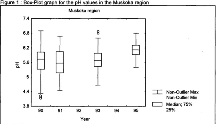
For the Muskoka region, data are available for 260 lakes and

4

years (1990, 1991, 1993 and 1995). Several missing values being present, only 782 observations are used for this regional trend detection analysis of pH values.

Fi ure 1 : Box-Plot

7.4

6.8 6.2 l 5.6 Q. 5

4.4

8

3.8 90 91 Muskoka region

B

92 93 Year ion 94 95

:::r::

Non-Outlier Max Non-Outlier Min [::J Median; 75% 25%

Figure 1 shows a couple of very low pH values in 1990 and a couple of very high values in 1993. However, these "outlier" values are not far enough to affect significantly the regional regression. Boxes and Whiskers show a tendancy for pH values to increase in time. The results of the regional regression support this fact :

n

R

2

Intercept estimate (year 0) Siope estimate

Initial value estimate (1990) Final value estimate (1995)

782 0.14 -2.675 0.0915/year 5.56 6.02

The regression is highly significant (p=0.0001). Figure 2 shows the regression line passing through the cloud of observations associated to each year. This plot shows the particularity of using linear regression with severallakes measured at a reduced number of years. Such a plot (data on only four levels of the independent variable) could suggest the use of analysis of variance to detect

(16)

changes in years instead of linear regression. The comparison of both approaches will be discussed in the final report.

7 ~ 6

J

::c a. 5 4 89 •

•

1 _•

1 90

Scatterplot of pH values in the Muskoka Region pH

=

-2.675+O.091*year+eps 1

_•

1

•

1 1

•

91 92 93 94 Year •

1

•

95 96

The regional regression shows a clear increasing trend for pH values in the Muskoka region. The increase of 0.09 uniVyear appears linear and no large outlier could affect significantly the conclusion of the regression. Figures 1 and 2 show that the variability of pH values between lakes seems to decrease in time. These graphs also suggest that lakes with very low pH in 1990 tend to increase more and could be the main reason for the significant regional regression. This hypothesis could be studied in more details.

Figure 3 presents the normal probability plot of the regional regression residuals. This graph supports the hypothesis that no large outliers affect significantly the conclusion of the regional regression.

(17)

4 3 Q) 2 ::J m 1

>

m E ₀ ~ 0 Z "0 _-1

~

Q) -2 Q. ~ -3 -4 -1.8 A/goma region -1.2

lot of residuals for H values in the Muskoka re ion Normal Probability Plot of Residuals

Muskoka region, pH values

-0.6 0

Residuals

0.6 1.2 1.8

For the Aigoma region, data are available for 256 lakes and 4 years (1988, 1992, 1994 and 1995). Several missing values being present, only 935 observations are used for this regional trend detection analysis of pH values.

Fi 8

7.5

7

6.5

6

J: Q.

_5.5

5 4.5 4

3.5

88

Box Plot for pH values in the Aigoma region

89 90 91 92 93 94 YEAR ion 95

:::r::

Non-Outlier Max Non-Outlier Min

c::J

Median; 75% 25%

(18)

Figure 4 shows that the non-outlier maximum changes less in time than the non outlier minimum. Boxes and Whiskers show a tendency for pH values to increase in time. The results of the regional regression support this fact:

n

R

2

935 0.06 0.00 0.064/year

5.77

6.09

The regression is highly significant (p=0.0001). Figure 5 shows the regression line passing through the cloud of observations associated to each year.

8 7.5 7 6.5 6

:a

5.5 5 4.5 4 3.5

1

•

Scatterplot of pH values in the Algoma region pH = -O.OO2+O.064*year+eps • YEAR • •

•

• 1

The regional regression shows a clear increasing trend for pH values in the Aigoma region. The increase of 0.06 unitlyear appears linear and no large outlier could affect significantly the conclusion of the regression. Figures 4 and 5 show that the variability of pH values between lakes seems to be more stable in time than in the Muskoka region. Like for the Muskoka region, these graphs suggest that lakes with low pH in 1988 tend to increase more and could be the main reason for the significant regional regression. This hypothesis could be studied in more details.

Figure 6 presents the normal probability plot of the regional regression residuals. This graph supports the hypothesis that no large outliers affect significantly the conclusion of the regional regression, but shows that the distribution of residuals has larger tails than the normal distribution.

(19)

lot of residuals for H values in the AI ion Normal Probability Plot of Residuals

pH values in the Aigoma region

4 3 G) 2 ~ ëii

>

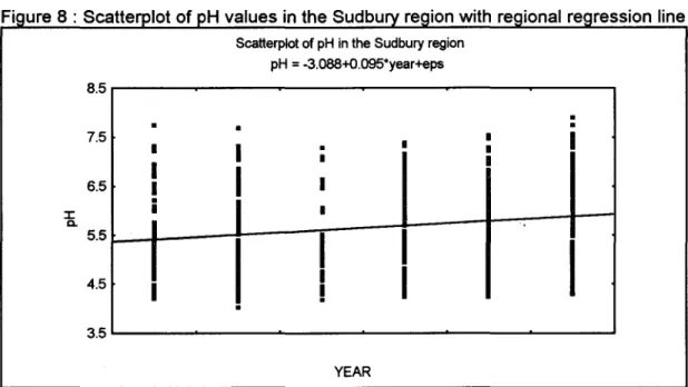
1 ëii E 0 .... 0 Z "C _-1 G) 1:) G) -2 0.. ~ -3 -4 Residuals Sudbury region

For the Sudbury region, data are available for 160 lakes and 6 years (1990 through 1995). Several missing values being present, only 755 observations are used for this regional trend detection analysis of pH values. Fi 8.5 7.5 6.5 J: Co 5.5 4.5 3.5

Box Plot of pH values in the Sudbury region

90 91 9~ YEAR 93 94 ion 95

::r:::

c::J

Median; 75% 25%

(20)

ln figure 7 boxes and whiskers show no clear trend pattern for pH values in the Sudbury region. The results of the regional regression, however, conclude to a significant positive trend :

n

R

2

755 0.03 -3.09 0.09 unitlyear 5.42 5.89

The regression is highly significant (p=0.0001). Figure 8 shows the regression line passing through the cloud of observations associated to each year.

8.5 • 7.5 1

1

6.5 ₁ • J: 1 Co. 5.5 4.5

1

3.5

Scatterplot of pH in the Sudbury region

pH = -3.088+O.095*year+eps

•

1

· _•

1

•

1

1 _• • YEAR

.

•

1

•

1

The regional regression line shows an increasing trend for pH values in the Sudbury region. The increase of 0.09 unitlyear appears linear and no large outlier could affect significantly the conclusion of the regression. Figures 7 and 8 show that the variability of pH values between lakes seems quite stable in time like in the Aigoma region.

Figure 9 presents the normal probability plot of the regional regression residuals. This graph supports the hypothesis that no large outliers affect significantly the conclusion of the regional regression, but shows that the distribution of residuals has larger tails th an the normal distribution.

(21)

lot of residuals for H values in the AI ion

Normal Probability Plot of Residuals pH values in the Sudbury region 4 3 CD 2 :::J cu

>

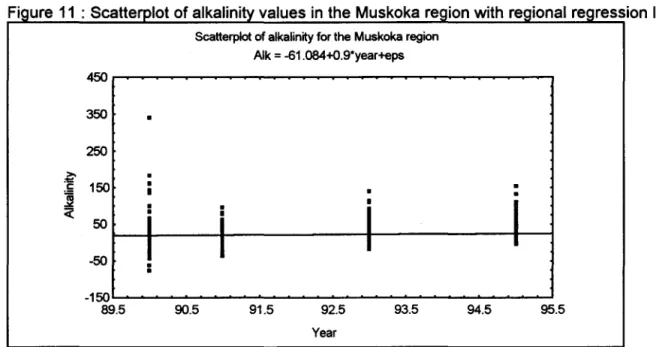
1 cu E 0 ~ 0 Z "0 _.-1 CD 1) CD -2 a. x W -3 0 -4 Residuals 2.2 Alkalinity values Muskoka region

For the Muskoka region, data are available for 260 lakes and 4 years (1990, 1991, 1993 and 1995). Several missing values being present, only 782 observations are used for this regional trend detection analysis of alkalinity values.

(22)

Fi ure 10 : Box-Plot ra h for the alkalinit values in the Muskoka re ion

Box Plot of alkalinity for the Muskoka region 450 350

..

250 ~ 150

1 ..

. 5

m

..

~

t

~

4

Cl 50 -50

::r:::

Non-Outlier Max

1

_{Non-Outlier Min} -150

CJ

Median; 75% 90 91 92 93 94 95 25% Year

Figure 10 shows several very high values in 1990 and a couple in 1993. These "outlier" values can affect significantly the regional regression. But the "nonparametric" boxes and whiskers do not show a clear trend pattern in the alkalinity values. The following results of the regional regression support this fact, while the positive slope suggests that the high outliers of 1990 do not affect significantly the conclusion of the regional trend detection :

n

R

2

782 0.004 -61.08 0.90 ppm/year 19.96 24.46

The regression is not significant (p=0.087). Figure 11 shows the regression line passing through the cloud of observations associated to each year, while figure 12 presents the normal probability plot of the regional regression residuals.

(23)

Fi ure 11 : Scatte lot of alkalinit values in the Muskoka re

>-""

.5 ~

«

450 350 250 150 50 -50 -150 89.5 •

·

• _•

•

Scatterplot of alkalinity for the Muskoka region Alk

=

-61.084+O.9*year+eps •

•

• i

1

90.5 91.5 92.5 93.5 Year

.

94.5 95.5

The regional regression scatterplot illustrates the non significance of the 0.90 ppm/year increase. Figures 10 and 11 show that the variability of alkalinity values between lakes seems to decrease in time. These graphs also suggest that lakes with very high alkalinity in 1990, do show smaller alkalinity values for the other years.

Figure 12 presents the normal probability plot of the regional regression residuals of the alkalinity values in the Muskoka region. This graph suggest non normal residuals but the results presented earlier should not be largely affected by this non normality. However, the very large(s) alkalinity value(s) in 1990 could be the reason why the regional regression does not conclude to a significant positive trend. 4 3 Q) 2 ::1 (ij 1

>

(ij E ₀ .... 0 Z -0 _-1 S ₍₎ Q) -2 Q.

.n

-3 -4 -150 -50

lot of residuals for alkalinit values in the Muskoka re ion Normal Probability Plot of Residuals

Alkalinity values in the Muskoka region

50 150

Residuals

o

(24)

A/goma region

For the Aigoma region, data are available for 256 lakes and 4 years (1988, 1992, 1994 and 1995). Several missing values being present, only 929 observations are used for this regional trend detection analysis of alkalinity values.

Fi ure 13 : Box-Plot ra h for the alkalinit values in the AI ion

th CI) ::J a; > ~

.s:

_a; ~

«

Box Plot for alkalinity in the Aigoma region

450 If 350 250 150 50 -50 -150

1:

If

ft

88 89 90 91 ~

ro

~ 95 YEAR

::r:::

c::::J

Median; 75% 25%

Figure 13 shows several very high values in 1988. These "outlier" values can affect significantly the regional regression. The "nonparametric" Boxes and Whiskers show a increasing trend pattern in the alkalinity values for the 1988 through 1994 period. The following results of the regional regression support this facto The high values of alkalinity in 1988 do not appear to affect significantly the conclusion of the regional trend detection :

n

R

2

929 0.02 -278.58 3.53 units/year 39.55 57.22

The regression is highly significant (p=0.0001). Figure 14 shows the regression line passing through the cloud of observations associated to each year, while figure 15 presents the normal probability plot of the regional regression residuals.

(25)

Fi ure 14 : Scatte 600 500 400 300 >.

""

200 .5 ]i :cc 100 0 -100 -200 •

·

· _•

•

Scatterplot of alkalinity in the Aigoma region Alk

=

-278.581 +3.535*year+eps

·

•

·

1 • YEAR • •

•

·

• • •

The regional regression scatterplot iIIustrates a 3.53 units/year increase. Figures 13 and 14 show that the variability of alkalinity values between lakes seems stable in time. These graphs also suggest that lakes with very high alkalinity in 1988, could also present high alkalinity values for the other years but this should be studied in more details to be sure that the same lakes are associated to high values from year to year.

Figure 15 presents the normal probability plot of the regional regression residuals for the alkalinity values in the Aigoma region. This graph suggests non normal residuals but the results presented earlier should not be largely affected by this non normality. However, the very large(s) alkalinity value(s) in 1994 could be a reason why the regional regression does conclude to a significant positive trend.

(26)

4 3 Q) 2 ::;, ïü 1

>

ïü E ₀ .... 0 Z "l:l _-1

~

_Q) -2 Q. x w -3 -4 Sudbury region

lot of residuals for alkalini values in the AI ion

Normal Probability Plot of Residuals Alkalinity in the Algoma region.

Residuals

o

0 0

o

For the Sudbury region, data are available for 160 lakes and 6 years (1990-1995). Several missing values being present, only 755 observations are used for this regional trend detection analysis of alkalinity values.

Fi ure 16 : Box-Plot ra h for the alkalinit values in the Sud bu ion Box Plot of alkalinity values in the Sudbury region

2000 1600

..

1200 II) Q) ;:, (ij

..

> ₈₀₀

..

~

..

1

.5

..

(ij

•

1 ₁

~ ₄₀₀

:cc

5 ~

..

0

~

l

;

0

~

::r:::

Non-Outlier Max Non-Outlier Min -400

CJ

Median; 75% 90 91 92 93 94 95 25% YEAR

(27)

Figure 16 shows several very high values in for ail years. These "outlier" values can affect significantly the regional regression in particular for the great variability they introduced in the data. The "nonparametric" boxes and whiskers show no clear trend pattern in the alkalinity values. The following results of the regional regression support this fact :

n

R

2

755 0.00 -388.71 4.92 units/year 54.34 78.96

Fi ure 17 : Scatte 2000 1600 _•

lB

1200 j

J

800 >-:t::! .5

•

~ 400 C( 0 -400

Scatterplot of alkalinity in the Sudbury region Alk = -388.714+4.923*year+eps

•

YEAR

• •

The regional regression scatterplot illustrates 4.92 units/year increase and its lack of significance compared to the large variability in the data. Figures 16 and 17 show that the variability of alkalinity values between lakes seems stable in time but appear quite large. These graphs also suggest that lakes with very high alkalinity in 1988, could also present high alkalinity values for the other years but this should be studied in more details to be sure that the same lakes are associated to high values from year to year.

Figure 18 presents the normal probability plot of the regional regression residuals for the alkalinity values in the Sudbury region. This graph suggests non normal residuals and the presence of very large outliers. The results presented earlier could be largely affected by this non normality and by the outliers. A nonparametric approach would be more appropriate to detect regional trend in the present case.

(28)

lot of residuals for alkalinit values in the Sudbu ion Normal Probability Plot of Residuals

Alkalinity in the Sudbury region

4r---~---~---~~--~--~---_. 3 QI 2 :::l

~

1ü

E

_o 0 Z " -1

J

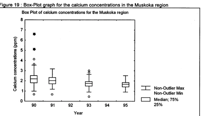
-2 -3 o o ~~---~---~---~---~---~ Residuals 2.3 Calcium concentrations Muskoka region

For the Muskoka region, data are available for 260 lakes and 4 years (1990, 1991, 1993 and 1995). Several missing values being present, only 790 observations are used for this regional trend detection analysis of calcium concentrations.

(29)

Figure 19 : B ox-PI ot graph for the ca clum concentrations 1 • ln . h M k k t e us 0 a reglon

Box Plot of calcium concentrations for the Muskoka region

8 7 If

-

E 6 _c. c.

-

th ₅ If c: 0 +:1 ca 4 0 ~ _Q) _..J~ ()

~

c: ₃

8

0 ()

~

E ₂ ::1 13

ïii

_:::c

_{Non-Outlier Max}

U ₁ 0 0 Non-Outlier Min 0

c::::J

0 Median; 75% 90 91 92 93 94 95 25% Year

Figure 19 shows several very hlgh values ln 1990 and a couple ln 1993. These "outller" values can

affect significantly the regional regression. The "nonparametric" boxes and whiskers show a clear decreasing trend pattern in the calcium concentrations. The following results of the regional regression support this fact:

n

R

2

790 0.16 13.31 -0.12 ppm/year 2.22 1.60

The regression is highly significant (p=0.0001). It must be kept in mind that the high outliers of 1990 can "artificially" inflate the negative trend amplitude. Figure 20 shows the regression line passing through the cloud of observations associated to each year, while figure 21 presents the normal probability plot of the regional regression residuals.

(30)

Fi ure 20 : Scatte lot of calcium concentrations in the Muskoka re 7

[6

8: III ₅ c:

~

4 ë

~

3

8

E ₂ ::J :Q IV () 0 89

Scatlerplot of calcium concentrations in the Muskoka region

Ca = 13.314-0.123*year+eps •

•

• • 90 91 92 93 94 Year •

·

• 95 96

The regional regression scatterplot clearly shows the significant decreasing trend of -0.12 ppm/year. Figures 19 and 20 show that the variability of calcium concentrations between lakes seems to decrease in time. These graphs also suggest that lakes with very high calcium concentrations in 1990, do show smaller concentrations for the later years. The latter result was also seen in the alkalinity values.

Figure 21 presents the normal probability plot of the regional regression residuals of the calcium concentrations in the Muskoka region. This graph shows the presence of possible high outliers, but except for a possible inflated trend slope, the results presented earlier should not be largely affected by these possible outliers.

Fi ure 21 : Normal 4 3 Q) 2 ::J iii 1

>

iii E ₀

...

0 Z ""0 _-1 Q) Ü Q) -2 0-x w -3 -4 -2 -1

lot of residuals for calcium concentrations in the Muskoka re ion

Normal Probability Plot of Residuals Calcium concentrations in the Muskoka region

o B

0 1 2 3

8

(31)

A/goma region

For the Aigoma region, data are available for 256 lakes and 4 years (1988, 1992, 1994 and 1995). Several missing values being present, only 917 observations are used for this regional trend detection analysis of calcium concentrations.

Fi ure 22 : Box-Plot ra h for the calcium concentrations in the AI ion

Box Plot of calcium concentrations in the Algoma region 14 12 If

-

E 10

₁

c. c.

-

II) ₈ c: 0 0 :;::1

8

RI 6 ~

~

$

Q)

@

(.)

~

c: ₄ 0 (.) E 2 ::J .(3

cu

_:::r:

_{Non-Outlier Max} 0 ₀ Non-Outlier Min -2

CJ

Median; 75% 88 89 90 91 92 93 94 95 25% YEAR

Figure 22 shows several very high values in 1988. These "outlier" values can affect significantly the regional regression. The "nonparametric" boxes and whiskers show a possible decreasing trend pattern in the calcium concentrations. The following results of the regional regression support this possibility:

n

R

2

917 0.02 11.13 -0.09 ppm/year 2.63 1.15

The regression is highly significant (p=0.0001). It must be kept in mind that the high outliers of 1988 can "artificially" inflate the negative trend amplitude. Figure 23 shows the regression line passing through the cloud of observations associated to each year, while figure 24 presents the normal probability plot of the regional regression residuals.

(32)

Fi ure 23 : Scatte 14 12 Ê ₁₀ Q,

.s

III ₈

~

6

~

8

4 E ₂ :::J :Q lU 0 () -2 • •

•

Scatterplot of calcium concentrations in the Algoma region Ca

=

11.131-O.095*year+eps

·

•

1

•

YEAR

•

·

The regional regression scatterplot clearly shows the significant decreasing trend of -0.09 ppm/year. Figures 22 and 23 suggest that lakes with very high calcium concentrations in 1988 could also present high alkalinity values for the other years but this should be studied in more details to be sure that the same lakes are associated to high values from year to year.

Figure 24 presents the normal probability plot of the regional regression residuals of the calcium concentrations in the Aigoma region. This graph shows the presence of a possible non normal distribution of the residuals, but the conclusion presented earlier should not be largely affected by this possible violation of the underlying normality assumption.

4 3 G) 2 :::J lii 1

>

lii E ₀ 0 Z 'U _-1

~

~ -2 x w -3 -4 0

lot of residuals for calcium concentrations in the AI ion

Normal Probability Plot of Residuals Calcium concentrations in the Aigoma region

(33)

Sudbury region

For the Sudbury region, data are available for 160 lakes and 6 years (1990-1995). Several missing values being present, only 755 observations are used for this regional trend detection analysis of calcium concentrations.

Fi ure 25 : Box-Plot ra h for the calcium concentrations in the Sud bu ion

Box Plot of calcium concentrations in the Sudbury region 35 30

..

-

E 25

..

Q. Q.

..

-

ln ₂₀ c:: 0 +:1

..

~ 15 c::

₁

1

Ci) ()

1

c:: ₁₀

..

0

1

0

8 g

()

9 ~

E

~

;:, ₅

~

'0

iü

:r:

_{Non-Outlier Max}

0 ₀

Non-Outlier Min

-5

c::J

Median; 75%

90 91 92 93 94 95 25%

YEAR

Like for the alkalinity values, figure 25 shows several very high values for ail years in the calcium concentrations. These "outlier" values can affect significantly the regional regression. The "nonparametric" Boxes and Whiskers show no clear trend pattern in the calcium concentrations. The following results of the regional regression support the absence of significant trend:

n

R

2

755 0.00 9.68 -0.07 ppm/year 3.68 3.35

(34)

Fi ure 26 : Scatte lot of calcium concentrations in the Sudbu re

Scatterplot of calcium concentrations in the Sudbury region Ca = 9.681-O.067*year+eps ~r---~---~---' 30

[25

S, III ₂₀

i

15

]

10 E 5 :J

~

₀ () -5 •

•

• •

1 ₁

•

1 YEAR

The regional regression scatterplot iIIustrates the absence of significant trend. Figures 25 and 26 suggest that lakes with very high calcium concentrations in 1990 could also present high alkalinity values for the other years but this should be studied in more details to be sure that the same lakes are associated to high values from year to year.

Figure 27 presents the normal probability plot of the regional regression residuals of the calcium concentrations in the Sudbury region. This graph shows the presence of a possible non normal distribution of the residuals and the presence of very large outliers. The conclusion presented earlier could be largely affected by this possible violation of two underlying assumptions.

Fi ure 27 : Normal 4 3 Q) 2 :J a; 1

>

a; E ₀ 0 Z ""C _-1 Q) "0 Q) -2 Q. dj -3 -4 0

lot of residuals for calcium concentrations in the Sud bu

Normal Probability Plot of Residuals Calcium concentrations in the Sudbury region

o

Residuals

o

8

(35)

2.4 Sulfate concentrations

Muskoka region

For the Muskoka region, data are available for 260 lakes and 4 years (1990, 1991, 1993 and 1995). Several missing values being present, only 790 observations are used for this regional trend detection analysis of sulfate concentrations.

Fi ure 28 : Box-Plot ra h for the sulfate concentrations in the Muskoka re ion Box Plot of sulfate concentrations for the Muskoka region

22

•

18 0

-

E 0-0- ₁₄ 0

-

1/) c 0 :;:1 ca ₁₀

E

0 ~

~

8

c

t

0 ₆ u

~

_:::l

2

_:::I:

Non-Outlier Max

(f)

•

Non-Outlier Min

-2

C1

Median; 75%

90 91 92 93 94 95 25%

Year

Figure 28 shows several very high values in 1990 and a couple in 1993. These "outlier" values can affect significantly the regional regression. The "nonparametric" boxes and whiskers show a decreasing trend pattern in the sulfate concentrations. The following results of the regional regression support this fact:

n

R

2

790 0.26 52.62 -0.51 ppm/year 6.93 4.39

The regression is highly significant (p=0.0001). It must be. kept in mind that the high outliers of 1990 can "artificially" inflate the negative trend amplitude. Figure 29 shows the regression line passing through the cloud of observations associated to each year, while figure 30 presents the normal probability plot of the regional regression residuals.

(36)

Fi ure 29 : Scatte lot of sulfate concentrations in the Muskoka re Ê

!

1/) c . 2

1!!

ë

~

CD

Ji!

_::::J CI) 22 18 14 10 6 2 -2 89

Scatterplot of sulfate concentrations in the Muskoka region S04 = 52.622-O.508*year+eps • •

•

1

_•

.

1

1 .

90 91 92 93 94 Year 1

•

95 96

The regional regression scatterplot cJearly shows the significant decreasing trend of -0.51 ppm/year. Figures 28 and 29 show that Iike for the three other parameters discussed, the variability of sulfate concentrations between lakes seems to decrease in time for the Muskoka region. These graphs also suggest that lakes with very high sulfate concentrations in 1990, do show smaller concentrations for the later years.

Figure 30 presents the normal probability plot of the regional regression residuals of the sulfate concentrations in the Muskoka region. This graph shows the presence of possible high outliers, but except for a possible inflated trend slope, the results presented earlier should not be largely affected by these possible outliers.

Fi ure 30 : Normal lot of residuals for sulfate concentrations in the Muskoka re ion

Normal Prabability Plot of Residuals Sulfate concentrations in the Muskoka region

4~---~---~~----~~----~---, 3 CD 2 ::1

~

ëii E (5 Z "0

j

0 -1 -2 -3 -4 -8 -4 o o

o

4 8 12 16

(37)

A/goma region

For the Aigoma region, data are available for 256 lakes and 4 years (1988, 1992, 1994 and 1995). Several missing values being present, only 942 observations are used for this regional trend detection analysis of sulfate concentrations.

Fi ure 31 : Box-Plot ra h for the sulfate concentrations in the AI ion

Box Plot of sulfate concentrations in the A1goma region 16 14

• -

_E 12 0 Cl. Cl.

-

II) 10 c: 0 +' l'CI ₈

-!

_(\) (.) 6 c:

~

0

~

(.)

.s

4 J! "3

:::c

Non-Outlier Max

en

2

₈

_{Non-Outlier Min} 0

CJ

Median; 75% 88 89 90 91 92 93 94 95 25%

YEAR

Figure 31 shows several very high values in 1988. These "outlier" values can affect significantly the regional regression. The "nonparametric" boxes and whiskers show a decreasing trend pattern in the sulfate concentrations particularly in the first three sampling years. The following results of the regional regression support this fact:

n

R

2

942 0.51 45.83 -0.45 ppm/year 5.60 3.36

(38)

Fi ure 32 : Scatte 16 14

l

12 .~ 10

i!

8 ë

i

6 CIl 4

i

~ 2

o

·

•

Scatterplot of sulfate concentrations in the A1goma region S04 = 45.829-0.447*year+eps

·

· _·

•

YEAR • 1

-•

The regional regression scatterplot clearly shows the significant decreasing trend of -0.45 ppm/year. Figures 31 and 32 show that like for the sulfate concentrations in the Muskoka region, the variability of sulfate concentrations between lakes seems to decrease in time in the Aigoma region.

Figure 33 presents the normal probability plot of the regional regression residuals of the sulfate concentrations in the Aigoma region. This graph shows the presence of possible high outliers, but except for a possible inflated trend slope, the results presented earlier should not be largely affected by these possible outliers.

lot of residuals for sulfate concentrations in the AI ion

Normal Probability Plot of Residuals Sulfate concentrations in the Aigoma region

4~---~---~---~--~---~ 3 Q) 2 ~

~

IV

E

0 o Z -0 -1

~

8.

-2 ~ -3 o o 4~--~---~----~---~ Residuals

(39)

Sudbury region

For the Sudbury region, data are available for 160 lakes and 6 years (1990- 1995). Several missing values being present, only 755 observations are used for this regional trend detection analysis of sulfate concentrations.

Fi ure 34 : Box-Plot ra h for the sulfate concentrations in the Sudbu ion

Box Plot of sulfate concentrations in the Sudbury region 24 If 20 If

-

_E If Cl. Cl. ₁₆ If

-

0 fi)

8

c 0

8

0 0 0 ~ 0 0 l'CI ₁₂ .1;:1

~

c CI) u c 0 ₈ u

~

0

§

:::::J ₄

e

:r:

Non-Outlier Max

en

₁

0 0

ft

_{Non-Outlier Min} 0 0

CJ

Median; 75% 90 91 92 93 94 95 25% YEAR

Figure 34 shows several very high and very low values for ail years. These "outlier" values can affect significantly the regional regression. The "nonparametric" boxes and whiskers show a decreasing trend pattern in the sulfate concentrations particularly between 1991 and 1994. The following results of the regional regression support the presence of a significant trend:

n

R

2

755 0.05 34.49 -0.28 ppm/year 9.41 8.01

(40)

Fi ure 35 : Scatte lot of sulfate concentrations in the Sudbu re Scatterplot of sulfate concentrations in the Sudbury region

S04 = 34.49-0.279*year+eps 24r---~----~---~---~----+_~ 20 ~ 16 1

·

•

·

•

• • • •

•

1

,2

~ 8r-1I---t----~----~----~----_LlJ

;jg ~ en 4

_•

·

•

• _•

1

•

·

•

o~----~~---~---+-~ YEAR

The regional regression scatterplot iIIustrates the significant decreasing trend of -0.28 ppm/year. Contrary to Muskoka and Aigoma regions, figures 34 and 35 do not sh w a decrease in time of sulfate concentrations variability.

Figure 36 presents the normal probability plot of the regional regressio residuals of the sulfate concentrations in the Sudbury region. This graph shows the presence of ossible high outliers, but the inflated variability introduced do not mask the significance of the tren slope.

lot of residuals for sulfate concentrations in the Sudbu ion Normal Probability Plot of Residuals

Sulfate concentrations in the Sudbury region 4 3 0 0 G) 2 ~ lU 1

>

lU E ₀ .... 0 Z "U _-1 G)

1

_x -2 w -3 -4 Residuals

(41)

(42)

(43)

(44)

(45)

(46)