Simulating climate over North America and atmospheric low-frequency variability using variable resolution modeling approach

UNIVERSITÉ DU QUÉBEC À MONTRÉAL

SIMULATING CLIMATE OVER NORTH AMERICA AND ATMOSPHERIC LOW-FREQUENCY VARIABILITY USING VARIABLE RESOLUTION

MODELING APPROACH

DISSERTATION PRESENTED

AS PARTIAL REQUIREMENT

OF THE DOCTORATE IN EARTH AND ATMOSPHERIC SCIENCES

BY

MARKO MARKOVIC

UNIVERSITÉ DU QUÉBEC À MONTRÉAL Service des bibliothèques

Avertissement

La diffusion de cette thèse se fait dans le respect des droits de son auteur, qui a signé le formulaire Autorisation de reproduire et de diffuser un travail de recherche de cycles supérieurs (SDU-522 - Rév.01-2006). Cette autorisation stipule que «conformément à l'article 11 du Règlement no 8 des études de cycles supérieurs, [l'auteur] concède à l'Université du Québec à Montréal une licence non exclusive d'utilisation et de publication de la totalité ou d'une partie importante de [son] travail de recherche pour des fins pédagogiques et non commerciales. Plus précisément, [l'auteur] autorise l'Université du Québec à Montréal à reproduire, diffuser, prêter, distribuer ou vendre des copies de [son] travail de recherche à des fins non commerciales sur quelque support que ce soit, y compris l'Internet. Cette licence et cette autorisation n'entraînent pas une renonciation de [la] part [de l'auteur] à [ses] droits moraux ni à [ses] droits de propriété intellectuelle. Sauf entente contraire, [l'auteur] conserve la liberté de diffuser et de commercialiser ou non ce travail dont [il] possède un exemplaire.»

UNIVERSITÉ DU QUÉBEC À MONTRÉAL

SIMULATION DU CLIMAT DE L'AMÉRIQUE DU NORD ET DE LA VARIABILITÉ DE BASSE FRÉQUENCE AVEC UNE APPROCHE DE

MODÉLISATION À RÉSOLUTION VARIABLE

THÈSE PRÉSENTÉE

COMME EXIGENCE PARTIELLE

DU DOCTORAT EN SCIENCES DE LA TERRE ET DE L'ATMOSPHÈRE

PAR

MARKO MARKOVIC

ACKNOWLEDGEMENTS

Since this is the end of the road for me as a PhD student, 1 find it very important to thank to the people that helped me to accomplish this journey.

My supervisor Dr. Hai Lin for being an excellent mentor guiding me through and helping me to transfuse ail my ideas into a scientific analysis. Hai's corrections of my written English were precious.

Dr. Colin G. Jones, my MSc supervisor, who inspired me to do PhD studies.

Dr. René Laprise and Dr. Laxmi Sushama for creating and maintaining CRCMD network and for fi nancial support. It was a great pleasure to study as a network membership, access to high-performance computer power facilitated my numerical experiments and many scientific conferences 1 attended enriched my knowledge and my connections with other colleagues world wide.

1 am very grateful to Mrs. Katja Winger. Numerical modeling is a piece of cake when Katja sits near you! Thanks a lot Katja! Many thanks to Dr. Bernard Dugas who answered thousands of questions 1 was asking during this time and on many valuable advices. Thanks a lot to my colleagues and friends: Jean-Philippe Paquin, Danahé Paquin-Ricard and Louis-Philippe Caron for: integrating me in Québec's society, aIl

cinq à sept evenings, support during hard days, and on number of translations from

English to French and vice versa.

1 need to acknowledge the effort of my grandparents Nada and Jovan for supporting me financially during my bachelor studies in Belgrade.

CONTENTS

LIST OF FIGURES xi

LIST OF SYMBOLS xxi

RÉSUMÉ xxiii

ABSTRACT xxv

LIST OF TABLES xv

LIST OF ACRONYMS xvii

INTRODUCTION 1

1. SIMULATED GLOBAL AND NORTH AMERICAN CLIMATE USING THE GLOBAL ENVIRONMENTAL MULTISCALE MODEL WITH A

VARIABLE RESOLUTION MODELING APPROACH .13

Abstract. 17

1.1 Introduction 18

1.2 Experimental Setup and Model Description 20

1.3 Seasonal means in winter and summer 22

1.3.1 Surface air temperature .23

1.3.2 Geopotential 25

1.3.3 Precipitation 26

1.4 Low and high frequency atmospheri,c variability 29

1.5 Interannual variability associated with tropical SST anomal y .30

x

2. DYNAMICAL SEASONAL PREDICTION USING THE GLOBAL ENVIRONMENTAL MULTISCALE MODEL WITH A VARIABLE

RESOLUTION MODELING APPROACH 57

Abstract. 61

2.1. Introduction 62

2.2. Model Setup and Experimental Design 65

2.3. The assessment of SGM signal-to-noise ratio 67

2.4. Composites of predicted seasonal mean anomalies for El Nino and La

Nina events 70

2.5. Simulated global mass circulation during ENSO 74

2.6. The forecast skill 76

2.6a. Category forecast 76

2.6b. RMSE and temporal correlation -:-:-:-.- 77

2.6c. PNA/NAO index 78

2.7. Summary 80

CONCLUSION AND FUTURE WORK .101

APPENDIX 107

LIST OF FIGURES

Figure Page

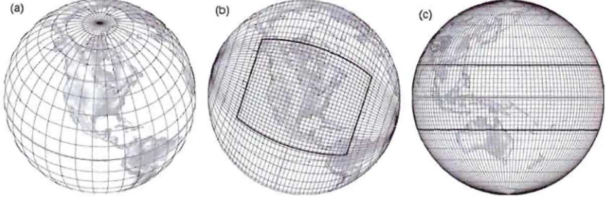
Il. The GEM model configurations: a) Global model with a uniform horizontal resolution; b) Limited Area Model, GEM-LAM; c) Variable resolution version with high-resolution domain centered over North

America. Kindly provided by Katja Winger. .11

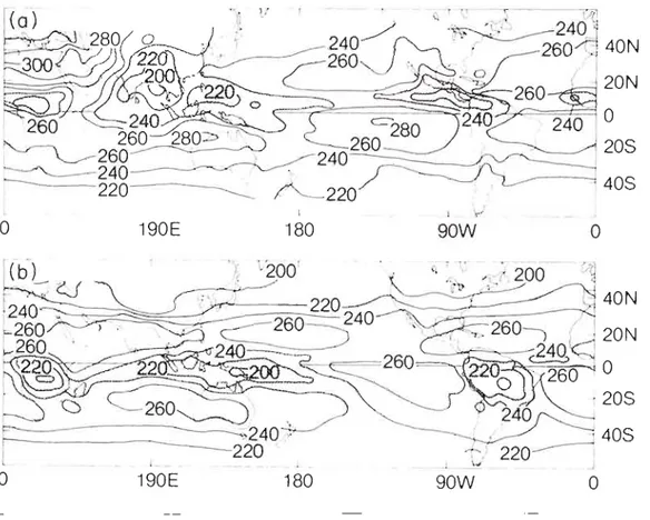
12. Mean seasonal outgoing longwave radiation measured by satellites: a)

winter season, b) summer season (taken from Philander, 1990) .12

1.1. Grid configurations: a) uniform grid, b) stretched grid with the area of interest over North America, c) stretched grid with the area of interest

over Equatorial Pacifie and East Indian Ocean ..40

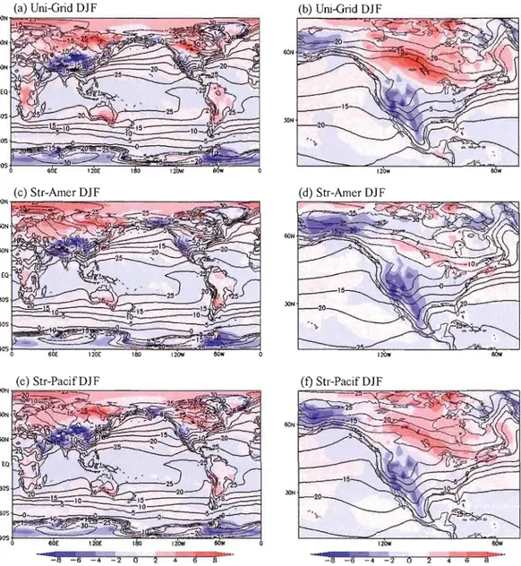
1.2. DJF season global and regional mean near surface temperature: a-b) Uni-Grid, c-d) Str-Amer, e-f) Str-Pacif. Mean tempe rature fields are represented with contour lines while biases against ERA40 with color

plots. Contour interval is five degree Celsius 41

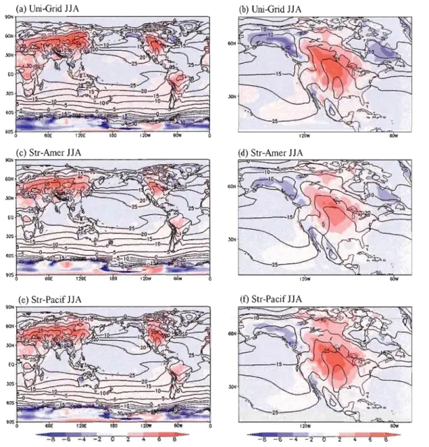
1.3. As in Figure 1.2, but for the JJA season ..42

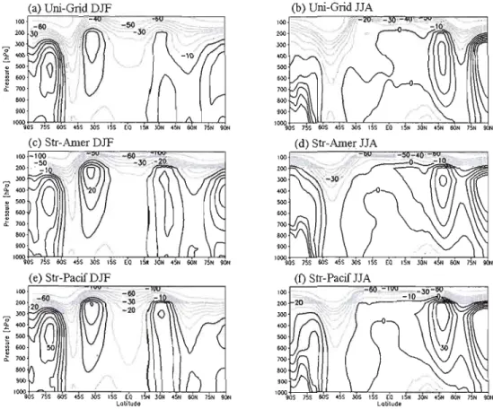
1.4. Vertical profile of zonal mean temperature bias over North America for DJF and JJA seasons against ERA40: a-b) Uni-Grid, c-d) Str-Amer, e-f) Str-Pacif. Values only above land have been taken into account.

Contour interval is one degree Celsius 43

1.5. DJF season near surface temperature standard deviation biases with respect to ERA40: a-b) Uni-Grid, c-d) Str-Amer, e-f) Str-Pacif. Contour interval is 0.5 degree Celsius, zero contour is removed. According to the F test, shaded areas reject the null hypothesis that standard

deviations are equal at 10% significance level. 44

1.6. As in Figure 1.5, but for the JJA season ..45

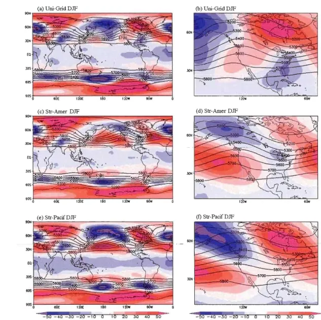
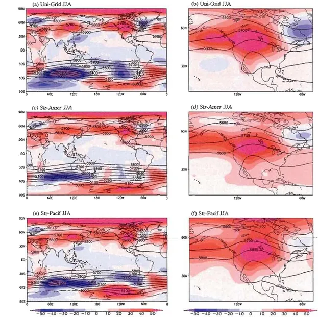
1.7. DJF season global and regional 500 hPa geopotential height: a-b) Uni-Grid, c-d) Str-Amer, e-f) Str-Pacif. Seasonal means are represented with contour lines while biases against ERA40 with color plots.

Contour interval is 100 geopotentiaJ meters ..46

1.8. Vertical profile of zonal mean geopotential height bias: a) Uni-Grid, DJF b) Uni-Grid, JJA c) Str-Amer, DJF, d) Str-Amer, JJA, e) Str-Pacif,

DJF, f) Str-Pacjf, JJA. Contour interval is 10 geopotential meters ..47

XII

1.10. Seasonal mean precipitation, DJF season: a-b) Uni-Grid, c-d) Str­ Amer, e-f) Str-Pacif. Mean precipitation fields are represented with contour lines while biases against CMAP observations with color plots.

Contour interval is 2 mm/day 49

1.11. As in Figure 1.10, but for the JJA season 50

1.12. Normalised frequency distribution of DJF and JJA monthly mean precipitation values, a-b) Tropical belt (200S-200N; 0°-360°), c-d)

North America (l5°-75°N, over land only) 51

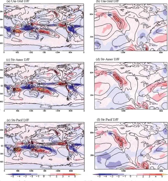
1.13. DJF 90-day high-frequency eddy rms: a) ERA40, b) Uni-Grid, c)

Str-Amer, d) Str-Pacif. Contour interval is 10 geopotential meters 52 1.14. As Figure 1.13, but for low-frequency eddy rms. Contour interval is 20

geopotential meters 53

1.15. OLR monthly mean anomalies. Spatial means over: a) Nino 3 [5°S_ SON; 150-900W], b) Nino 4 [5 0S-S ON; 1600E-1500W], c) Region 1 [5 0S-S ON; 11O-1600E], d) Region 2 [5 0S-S ON; 60-1100E]. Textual insets stand for the correlation coefficients between the respective

models configurations and observations 54

1.16. Linear regression of one standard deviation SST first principal component to DJF 500 hPa geopotential height: a) ERA40, b) Uni-Grid, ~) Str-Amer, d) _Str-Pacjf. Units are ingeopotential decametre.s corresponding to one standard deviation of equatorial Pacifie SST PC1.

Shaded areas are statistically significant at 5% level. 55

1.17. As Figure 1.16, but regressed to DJF T2m. Units are in degrees Celsius corresponding to one standard deviation of equatorial Pacifie SST PC1. Solid black lines encompass areas that are statistically significant at 5%

level 56

2.1. Comparison of geopotential height at 500 hPa external (signal), internai (noise) variances and their ratio (signal-to-noise) between the three model configurations. Contour intervals are given on the right hand side for the each figures row. Units for external and internai variances are gpdm2. Shaded area reject the null hypothesis that external and internai v~ri~n('p~ ~rp ~~J..l~! ~?.!,:~!!~!~tj !C): ~!~!~~!~S~! ~:;~::i::::c~ ~~ l)~%. Corresponding F test is defined as F=Y· Ve / Vi, where Y is the

ensemble size 86

2.2. As in Figure 2.1 but for T2m. The nul! hypothesis of external and internai variances being equal at 99% is rejected when signal-to-noise ratio is greater than 0.31. Units for external and internai variances

xiii

2.3. Seasonal mean [a) ERA40] and ensemble seasonal mean [b) Uni-Grid, c) Str-Amer, d) Str-Pacif] T2m calculated for El Nino years. In degrees

Celsius 89

2.4. As in Figure 2.3 but for La Nina years 90

2.5. Seasonal mean [a) ERA40] and ensemble seasonal mean [b) Uni-Grid, c) Str-Amer, d) Str-Pacif] geopotential height anomalies at 500 hPa calculated for El Nino years. Units in gpm. Shaded are the values

greater than 60 and lesser than -60 gpm 91

2.6. As in Figure 2.5 but for La Nina years 92

2.7. Nonlinear component of the seasonal mean [a) ERA40] and ensemble seasonal mean [b) Uni-Grid, c) Str-Amer and d) Str-Pacif] geopotential height anomaly at 500 hPa estimated as a sum of warm and cold

composites. Units in gpdm 93

2.8. Seasonal mean [a) ERA40] and ensemble seasonal mean [b) Uni-Grid, c) Str-Amer, d) Str-Pacif] meridional stream function anomalies for El Nino Composites. Units in 1010 kg/s. Shaded areas cover positive

contour values 94

2.9. As in Figure 2.8 but for La Nina composites 95

2.10. Percentage of correct forecast calculated from the preselected categories of above, below or near normal climate (see text for details): a) Uni-Grid, b) Str-Amer, c) Str-Pacif. Solid black lines encompass areas that are statistically significant at 5% level according to Monte Carlo approach. The numbers on the upper part of the panels represent the percentage of the statistically significant area within the PNA region

and globally 96

2.11. As Figure 2.10, but for T2m. The numbers on the upper part of the panels represent the percentage of the statistically significant area over

North America and globally, land only 97

2.12. Geopotential height at 500 hPa skill scores, RMSE (contour lines) and temporal correlation (shaded areas) statistically significant at 5% level according to t test for: a) Uni-Grid, b) Str-Amer, c) Str-Pacif. RMSE

units in gpdm. Contour interval is one gpdm 98

2.13. T2m skill scores, RMSE (col or) and temporal correlation (contour line) statistically significant at 5% level according to t test for: a) Uni-Grid, b) Str-Amer, c) Str-Pacif. RMSE units in degrees Celsius. statistically significant at 5% level according to t test for: a) Uni-Grid, b) Str-Amer,

XIV

2.14. The first two modes of ERA40 geopotential height at 500hPa REüF: a) REüF1, b) REüF2. Units correspond to one standard deviation of the

respective principal component. The contour interval is 10 gpm 100 Al. a) The first EüF of AMIP 2 SST, values are in degrees Celsius

corresponding to one standard deviation of the first principal component, contour interval is 0.2°C; b) principal component of the

first EüF of AMIn SST, normalised units .109

A2. Percentage of correct forecast calculated from the preselected categories of above, below or near normal c1imate for precipitation fields: a) Uni­ Grid, b) Str-Amer, c) Str-Pacif. Solid black lines encompass areas that are statistically significant at 5% level according to Monte Carlo

approach 110

A3. Precipitation skill scores, RMSE (color) and temporal correlation (contour line) statistically significant at 5% level according to t test for:

a) Uni-Grid, b) Str-Amer, c) Str-Pacif. RMSE units in mmday-1 111 A4. Wavenumber-frequency power spectrum for 10oS-lOoN band averaged

precipitation field calculated for the first 240 days of each year within 1997-2006 period, a) GPCP observations, b) Uni-Grid, c) Str-Amer, d) Str-Pacif. Positive (negative) frequency values correspond to the

LIST OF TABLES

Table Page

1.1. Near surface tempe rature spatial mean differences and rmse for the three model configurations with respect to ERA40 for winter and summer seasons, calculated over continental North America. Region 1: 15°N­ 35°N, region 2: 35°N-55°N, region 3: 55°N-75°N and total: 15°N­

75°N. Units are degrees Celsius 38

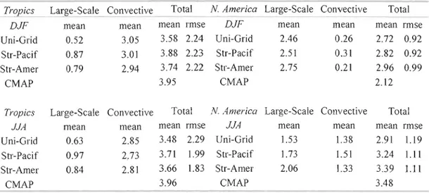
1.2. Spatial mean differences and rmse of the three models configurations simulated precipitation against CMAP data for winter and summer. Tropical belt (200S-200N; 0°-360°), N. America (15°-75°N, over land

only). [n mm/day .38

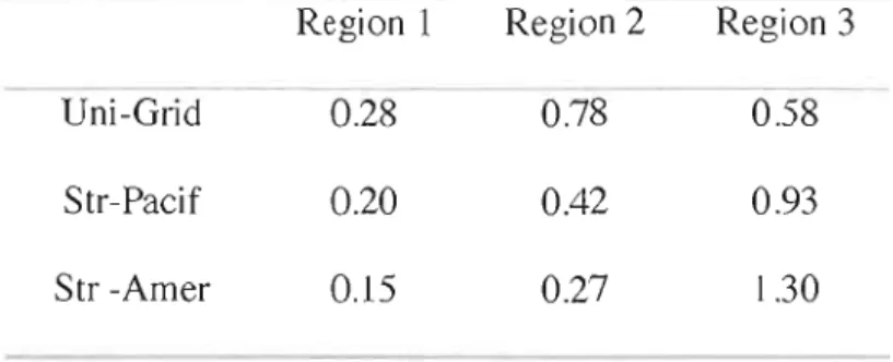
1.3. Absolute spatial mean differences between the three models configuration and ERA40 according to the resul ts presented in Figure 1.16 for the three selected regions. Units are geopotential meters

corresponding to one standard deviation of equatorial Pacifie SST PC1 .39 1.4. Absolute spatial me an differences over continental North America

between the three models configuration and ERA40 according to the results presented in Figure 1.17. Units are degrees Celsius corresponding to one standard deviation of equatorial Pacifie SST PC 1.

Region 1: 15°N-35°N, region 2: 35°N-55°N, region 3: 55°N-75°N 39 2.1. Absolute spatial mean differences over continental North America

between the three model configurations and ERA40, for T2m anomalies, in degrees Celsius. Spatial correlation, in percent, is calculated for the entire continent. Region 1: 15°N-35°N, region 2:

35°N-55°N, region 3: 55°N-75°N and total: 15°N-75°N 83

2.2. Absolute spatial mean differences over PNA region between the three model configurations and ERA40, for geopotential height at 500 hPa anomalies, in geopotential meters. Spatial correlation, in percent, is also

calcuJated for the PNA region 83

2.3. RMSE and temporal correlation skill scores between the model configurations and ERA40 reanalysis. RMSE units are geopotential meters and degrees Celsius. Area of statistically significant temporal correlation at 5% level is calculated relative to the domain of interest.

T2m skill scores are calculated only over land 84

AMIn ARPEGE BB CFCAS CMAP CMC CRCMD CSIRO DJF DJFM ENSO EOF ERA40 EW GCM GPCP GEM GEM-CLIM LIST OF ACRONYMS

Atmosphere Model Intercomparison Project 2 Action de Recherche Petite Echelle Grande Echelle Big Brother experiment

Canadian Foundation for Climate and Atmospheric Sciences

CPC Merged Analysis of Precipitation Canadian Meteorological Centre

Canadian Regional Climate Modeling and Diagnostics

Commonwealth Scientific and Research Organization

December-January-Fe bruary

December-January-February March El Nino Southern Oscillation Empirical Orthogonal Function

European Reanalysis, covering 40 years East-West

Global Climate Model

Global Precipitation Climatology Project Global Environmental Multiscale Model

Global Environmental Multiscale Model in Climate mode

xviii GEM-LAM GEOS ISBA ITCZ JFM JJA LAM LBC LMDz

MIO

MJO NA NAO NCAR NCEP NS NSERC OLR PC PNA

Global Environmental Multiscale Model in Limited Area Approach

Global Earth Observing System

Interaction Soil-Biosphere-Atmosphere Inter Tropical Convergence Zone January-February-March

June-July-August Limited Area Model

Lateral Boundary Conditions

Laboratoire de Météorologie Dynamique Markovic et al., 2010

Madden Julian Oscillation North Atlantic

North Atlantic Oscillation

National Centre for Atmospheric Research National Centre for Environmental Prediction North-South

Natural Science and Engineering Research Council of Canada

Outgoing Longwave Radiation Principal Component

xix

RCM rmse rms SF SGM SGMIP SO SST Str-Amer Str-Pacif SURF TOA Uni-Grid

Regional Climate Model Roor mean square error Root mean squares Stream Function Stretched Grid Model

Stretched Grid Model Intercomparison Project Southern Oscillations

Sea Surface Temperatures

Stretched Grid Model with a high resolution grid placed over North America

Stretched Grid Model with a high resolution grid placed over Tropical Pacifie and East Indian Ocean

Surface

Top of the Atmosphere Uniform Grid

LIST OF SYMBOLS dxj F g GZ500 M

Horizontal distance between the two adjacent grid points

Ratio between the external and internai sum of squares

Gravitational acceleration Geopotential height at 500 hPa Total ensemble mean

Ensemble mean calculated separately for each ENSO season N

p

r R Number of years Pressure Stretching factor Earth 's mean radius

T2m Near surface temperature

v

Temporal and zonal average of the meridional velocity

Variance of external sources Variance of internai sources

y

_{Ensemble size}

Latitude

RÉSUMÉ

Les modèles climatiques à résolution variable, dont les modèles à grille étirée, permettent l'utilisation d'une fine résolution sur les zones d'intérêts, résolution hors d'atteinte pour les modèles mondieux. L'approche à résolution variable possède aussi l'avantage d'une grande efficacité concernant l'utilisation des ressources de calcul. L'absence dans de tels modèles de conditions aux frontières latérales représente aussi un atout pour la simulation du climat à l'échelle mondialee mais aussi régionale.

Cette étude à pour objectif d'évaluer la simulation du climat nord-américain à l'aide de la configuration à résolution variable du Global Multiscale model (SGM­

GEM) afin d'évaluer les bénéfices respectifs de localiser la zone de haute résolution localement, au-dessus de l'Amérique du Nord, ou au-dessus du Pacifique équatorial, région de forçage important pour la variabilité du climat nord-américain:

De plus, nous avons étudié les bénéfices potentiels de l'approche à résolution variable avec une emphase sur les téléconnections entre les anomalies de la température de surface de la mer et le climat nord-américain. Nous avons évalué des ensembles de simulations de prédiction saisonnière des mois hivernaux d'années ENSO sélectionnées. Les ensembles comprennent 10 membres pour chacune des configurations du SGM-GEM présentées précédemment.

En comparaison avec la version de GEM à grille uniforme (simulation de référence), il a été démontré que les simulations utilisant l'approche

à

résolution variable, pour chacune des configurations, reproduisent généralement mieux les observations au-dessus de leurs zones à haute résolution, malgré une détérioration de certaines variables. De plus, certaines erreurs systématiques observées dans la simulation de référence demeurent présentes dans les simulations du SGM-GEM. La localisation de la zone de haute résolution au-dessus d'une zone de forçage important (Pacifique équatorial) ne semble pas provoquer une amélioration nette du climat au­ dessus de la région d'intérêt (Amérique du Nord) pour les simulations climatiques multi-annuelles. Chacune des configurations du SGM-GEM testée simule des téléconnections réalistes associées au mode dominant de la variabilité interannuelle des anomalies de la SST du Pacifique équatorial.

Les simulations SGM-GEM avec la zone de haute résolution au-dessus du continent nord-américain reproduisent avec plus de précision les anomalies de la température près de la surface et obtiennent de meilleures résultats d'analyse (skill scores) pour l'ensemble du continent. Par contre, aucune configuration ne semble

indiquer une amélioration claire de la simulation du géopotentiel à 500hPa au-dessus du continent. Les erreurs dans la prévision du rapport signal-bruit est le résultat des non-linéarités des réponses aux deux composites ENSO et interprétées comme le résultat des incohérences des réactions du modèle atmosphérique aux différentes anomalies de la température de surface de la mer. Les résultats de cette étude ne peuvent démontrer que, dans un contexte de prédiction saisonnière, l'approche à

xxiv

résolution variable représente un avantage en comparaison à l'approche à résolution uniforme. L'amélioration de la prédiction des champs de surface produite par les simulations SGM-GEM semble être reliée à une représentation plus précise du bilan radiatif de surface et à d'autres processus de surface directement liés au schéma de surface utilisé.

AB8TRACT

Variable resolution models (also known as stretched grid models, [SGMsD offer the possibility of using a very fine horizontal resolution over a specifie geographical region of interest, a resolution that cannot be attained using global climate models. A variable grid approach is found to be very efficient in terms of computational time and resources. The fact that SGMs do not suffer from the lateral boundary condition problem makes variable resolution technique a valuable tool for regional and global climate modeling.

In this work we evaluate variable resolution Global Environmental Multiscale model (SGM-GEM) simulations with increased horizontal resolutions over the North American continent and over the tropical Pacifie in order to determine whether it is better to increase the model resolution locally (North America) or over a particular remote region of important boundary forcing (the tropical Pacifie), with respect to the target region of North America.

Moreover, we investigate possible benefits of the variable resolution modeling technique in representing regional climate over North America, with an emphasis on atmospheric teleconnection patterns related with sea surface temperature (SST) anomalies. Mainly over the North American continent, we evaluate ten-member ensemble seasonaL forecast predictions for each of the aforementioned SGM-GEM settings in forecasting four winter months of selected ENSO years.

It is found that each SGM-GEM integration better simulates the observations over its respective highly resolved domain than the low resolution uni-grid run (control run). Despite of overall decent performances, sorne evidence of result deterioration over the high-resolution zone is also observed. Sorne systematic errors seen in the control run remain in the SGM simulations. Little evidence is found that an increased resolution over a region of important boundary forcing has a significant impact on the targeted remote region (North America) through the multiyear climate simulations. Both SGM simulations showed a realistic teleconnection patterns associated to the dominant mode of SST interannual variability in the tropical Pacifie. Simulation with increased resolution over North America showed most aceurate near surface temperature seasonal ensemble-mean anomalies and skill score over the matching continent. Considering geopotential height at 500hPa, there is no model configuration that consistently shows more accurate results over the continent. Erroneous forecast signal-to-noise ratio is linked to the simulated non-linearity between the two ENSO composites and perceived as model 's inconsistent response to the boundary conditions. There is not enough evidence indicating that the SGM has a clear advantage in seasonal prediction comparing to the uniform grid approach. The fact that the near surface temperature prediction is improved with the SGM is related to the better represented surface radiation balance and other surface processes (controlled by the surface scheme).

INTRODUCTION

The main goal of this research is to investigate possible benefits of variable resolution modeling technique in representing climate over North America, with an emphasis on atmospheric teleconnections. Considering sea surface temperature (SST) anomalies to be one of the prevalent forcing in the equatorial Pacifie influencing even mid-latitudes (Horel and Wallace, 1981; Trenberth et al., 1998), this study investigates the cOI1nection between SST and dominant atmospheric patterns using variable resolution climate model. Moreover, using seasonal prediction experiments, this study investigates relation between tropical SSTs and extratropical circulation.

Developed in the 1970s, variable resolution global climate models, including stretched grid models (SGMs), have been used at the Canadian Meteorological Centre since early 1990s (Côté et al, 1993, 1997). Météo-France performed its first operational forecast using this approach in the mid 1990s (Déqué and Piedelièvre, 1995), while approximately at the same time the Goddard Earth Observing System (GEOS) SGM was developed (Held and Suarez, 1994). Beside these institutions, variable resolution technique has also been widely used in Laboratoire de Météorologie Dynamique (LMDz), France, (Li and Conil, 2003); Australian Commonwealth Scientific and Research Organization (CSIRO), (Lai et al., 2008) and at The National Centre for Atmospheric Research (NCAR), (Fox-Rabinovitz et al., 2006). The method of variable resolution offers the possibility of using very fine horizontal resolution over a specifie geographical region of interest, a resolution that cannot be attained using global climate models (GCMs). Telescoping from the coarser to the highly resolved horizontal grid boxes SGM technique enables consistent propagation of signais and interaction between meteorological phenomena of regional and global scales mostly through the preservation of global circulation (Fox-Rabinovitz et al., 2005). Furthermore, a variable grid approach is found to be

2

very efficient in terms of computational time and resources. The fact that SGMs don't suffer from the lateral boundary condition problem like regional climate models (RCMs), makes variable resolution technique a valuable tool for regional and global climate modeling.

The Global Environmental Multi-scale model presently used at the Meteorological Service of Canada supports several operational options: Global Climate Model with a regular/uniform latitude-longitude grid, global-variable resolution grid with possible higher resolution over selected domain of interest (also caUed stretched grid model, SGM), and a limited area model (LAM) option (see Figure Il).

The latter two options enable high-resolution simulation over limited geographical areas. A regional climate model, GEM-LAM suffers from aIl imperfections in treating Lateral Boundary Conditions (LBC) that can be provided either by GCMs or various reanalysis or observational products (e.g. ERA40, NCEP). Sharp transition in resolution from LBC to LAM at the lateral boundaries, spin-up time, temporal interval to LBC input, diurnal cycle of LBC (if taken from observations) are sorne of the issues that have to be addressed when using LBC in regional climate modeling (Giorgi and Mearns, 1999). Another approach to avoid these problems, associated with one-way nesting is the spectral nudging approach

(Von Storch et al., 2000). In the experiment called "Big Brother" (BB), Denis et al., (2002) filtered small-scale meteorological information obtained from the BB-RCM run and subsequently used that information to feed another RCM, of smaller domain,

able to develop its own fine-scale features and to reproduce the time mean and variability of a number of meteorological fields comparable to the RCM with the larger domain.

3

As an alternative t<J LAMs nested-grid approach, SGMs employa two-way

nesting strategy, which allows for exchanges of meteorological information and communication betweens different resolution zones. Within a GCM, a regular latitude-longitude region is selected with a fine resolution, usually few times finer than that of the GCM. Just outside of this fine-resolution domain, the grid is stretched in both directions, usually with a constant stretching factor of:

(1)

between the adjacent grid boxes. According to Fox-Rabinovitz et al. (2000), r is most efficient if it varies by 5-10%, enabling fine meso-scale resolution over the region of interest. This stretching factor is applied until the horizontal resol ution between the grid points reaches sorne predetermined coarse resolution. The most important advantage of SGM approach is the possibility to assemble a multi-year simulation without the need of the periodic input on its boundaries from a driving GCM or analysis, and consistent interactions between global and regional scales of motion (Fox-Rabinovitz et al., 2006). For regional c1imate simulation experiments, Fox­ Rabinovitz et al. (2000,2001) calculated that, compared to a uniform GCM control run, SGM was 4 to 9 times more computationally efficient for moderate stretching zones and to 16 times for large stretching zones. Therefore, utilized as a GCM, stretched grid modeling approach can provide very successful c1imate simulations on the regional scales.

Targeting the c1imate over Europe, Déqué and Piedelièvre (1995) compared 10-year simulations of variable resolution version of Action de Recherche Petite Echelle Grande Echelle (ARPEGE) c1imate model with two global-uniform ARPEGE simulations of different horizontal resolutions. Their results showed that with an increase of horizontal resolution wintertime mean general circulation improves.

4

Considering near surface temperature and precipitation biases over Europe, an improvement was observed in both high-resolution simulations (i.e. variable resolution and the high-resolution global-uniform simulation). The authors suggested a variable resolution approach as a valid alternative to model nesting.

The Stretched-grid Model intercomparison project (SGMIP) (Fox-Rabinovitz et al., 2006) revealed many advantages in using variable resolution approach. Evaluating several SGMs (e.g. GEM, Goddard Earth Observing System [GEOS], Action de Recherche Petite Échelle Grande Échelle [ARPEGE]) mostly through the ensemble technique for multi year simulations, they concluded that the multi model ensemble generally represents seasonal and interannual variability very weil, with time evolution, seasonal differences and variations being close to observations or reanalyses. An important characteristic of their work was the fact that high-resolution regional forcing allows orographically induced precipitation and other small-scale features to be weil represented within the area of interest. Better resolved model dynamics_ and enhan_ced stationary boundary forcing stemm-ing from the fine resolution orography and land-sea differences was a major benefit from a stretching technique.

In order to enhance climate information over the region of Fiji islands Lai et al. (2008) used a variable resolution version of the CSIRO climate mode!. A climatological study with a dynamical downscaling up to 8 km of horizontal resolution was performed over the region of interest. The model showed fine results in simulating annual cycles of maximum and minimum surface air temperature and

Constraining the analysis to the periods of important SST forcing (e.g. El Nino) a models capability to separate the impact of moderate to strong El Nino to the Fiji rainfall was confirmed.

5

Numerous studies have shown the strong link between the anomalous tropical Pacifie SST and the interannual variability of the extratropical circulation (e.g. Trenberth et al., 1998). Large-scale atmospheric motions in the regions of Tropical Pacifie and East Indian Ocean correspond directly to thermally dri ven circulations. The warm and moi st air rises above the regions where the SST is highest and subsequently subsides poleward and eastward of these regions, where SST is cold. This atmospheric motion is also known as the Hadley circulation. Gill (1982) describes this motion as a diabatic heating of the air located directly above the Intertropical Convergence Zone (ITCZ) followed by a poleward diverging and subsidence on both sides of the ITCZ. Since the air parcel has both meridional and zonal velocity components, rising air will also have zonal divergence, subsiding on adjacent regions, a process known as the Walker circulation (Bjerknes, 1966).

During the Boreal summer, the northern branch of the ITCZ is very strong and developed ail across the tropical Pacifie with intense convection over north India. During this season, regions in Pacifie and East Indian Ocean between lOoN and 15°N receive their maximal rainfall. Shifting to winter season the region of intense convection moves towards the southeast, intensifying the southern branch of the ITCZ and weakening its northern counterpart. Figure 12 (taken from Philander, 1990) represents mean outgoing longwave radiation (OLR) obtained from satellite measurements for winter (Fig. 12a) and for summer (Fig. 12b) season. OLR is a good indicator of deep convection, thus regions in the tropics with values less than 240 Wm-2

corresponding to high cloud tops at low temperature, have strong convection and receive heavy rainfall. Shifting of the convection centers, and therefore ITCZ, towards southeast can be c1early seen in Figure 12. Rainfall in the equatorial regions depends mostly on the presence of the ITCZ and maximum precipitation occurs in March and April, when ITCZ shifts southward (Halpern and Hung, 2001). During the late spring, the northern

ncz

branch strengthens again and convection regions move westward and toward the equator.

6

The example of thermally driven circulation in the Indian Ocean is the monsoon circulation, which blows from the regions of high surface pressure towards the convective regions of low surface pressure. As the regions of high convection shift with seasons, the direction of the surface winds shifts also. Southwest monsoon is active within May-October seasons (brings heavy rainfall to the Indian sub continent) while northeast monsoon prevails within December-March. The period of transition is from April to November (Philander, 1990).

The Southern Oscillation is the principal mode of interannual variability in the tropics and shows as a difference in sea-level pressure between western tropical Pacific/Northern Indian Ocean and eastern tropical Pacifie (Darwin and Tahiti). During its El Nino phase, high surface pressure anomal y is established over the western and low pressure anomal y over the eastern tropical Pacifie with warm surface waters and heavy rainfall in the central and eastern tropical Pacifie. La Nina SO phase is, conversely, characterized by low pressure anomaly in western and high surface pressure in theeastern tropical Pacifie with -intense surface win<:ls, low SST and weak rainfall in eastern and central Pacifie. Philander (1990) has shown that in the region of tropical Pacifie where the SO describes a major part of their variance, meteorological variables such as SST, sea level pressure, geopotential (200hPa thickness), precipitation, etc. are highly correlated on large time scales, making SO the prevalent atmospheric pattern in the region. The peak of SO is on the time scale of three years, but the irregularity of oscillations makes different meteorological variables peak on time scale of two to ten years. The most studied extratropical response to the El Nino forcing is the PNA teleconnection pattern (Wallace and Gutzler, 1981). This signal accounts for a significant part of the variance of interannual variability in the midlatitude North Pacifie and North America, and is a dominant source of skill for seasonal forecasts (Zwiers, 1987; Derome et al., 2001).

7

Besides the Pacifie and Indian Ocean basins, changes in SST gradient in the equatorial Atlantic can influence the position of the ITCZ which has a direct impact on the interannual variability and predictability of precipitation over Brazil and western Africa (Rowell, 1995).

The possibility of seasonal forecasting stems from two important sources of predictability: initial conditions and boundary conditions. On seasonal timescales boundary conditions have a more prevalent influence on model simulations than the initial conditions whose importance generally weakens with time after a simulation is initiated (Goddard et al., 2001; Brankovic and Palmer, 2000). However, initial conditions related to the land surface description (e.g. soil moisture, snow, landscape specification, etc.) may have a significant influence on the seasonal prediction results (Pielke, 1999; Brankovic and Palmer, 2000). The study of Liu and Avisar (1999) revealed the importance of the soil moisture initial conditions even 200 days after the onset of a GCM simulation. The dominant boundary forcing signal for seasonal prediction is provided by SSTs. Evolving slowly, they have significant influence on the tropical and extra tropical atmosphere by redistri buting surface heating, convection and low-Ievel fields. Land-surface is also a very important boundary condition but with the time scales of the surface processes much less than the timescales of the ocean (Goddard et al., 2001).

Among the first attempts to quantify variability of skill and general use of long-range and seasonal timescale forecasts was that made by Livezey (1990). By evaluating the National (United States) Weather Service forecast, it was found that higher skill over North America is related to specifie seasons (e.g. winter, early spring), varying with particular variable and geographical location. This study is in accord with the linear-statistical seasonal forecast performed by Barnston (1994) using the SST and North Hemispheric geopotential height at 700 hPa as predictor fields. They also found higher skill associated with ENSO events occurring in winter

- - - - -8

season through spring, and in the Pacifie and North American regions. In a warm ENSO event the largest positive temperature anomalies are linked to the region of southwestern Canada.

Frederiksen et al. (1997) pelformed multi ensemble GCM simulations, forced with persisted SST anomalies, in order to study 1997/1998 ENSO event. Over the tropical belt, they reported significant skill in forecasting seasonal anomalies of precipitation, sea-Ievel-pressure, 200 hPa geopotential height and near surface temperature. At higher latitudes systematic skill was found only in near surface temperature and 200 hPa geopotential height. Important teleconnection patterns such as the PNA and south hemispheric wave train were also skillfully forecasted.

Graham et al. (2000) used multi-year multi-ensemble GCMs simulation in order to assess seasonal predictability and skill over different geographical regions. The higher skill was found over the tropics in ail seasons, while over the Northern Hemispheric extratropics skill peaked in spring. Over North America skill was ~ound_ . in winter season 850-hPa temperature and precipitation. They related this result to the enhanced winter predictability of the PNA mode during Pacifie cold and warm events. During non-ENSO events, they reported similar skill for the European and North American continents. Moreover they tested a GCM performance forced by persisted SST anomaly approach and found retained skill compared to model skill forced with observed SST. They suggested persisted SST anomal y approach a viable method for a real-time seasonal forecast.

Chang et al., (2000) tested the influence of initial and boundary conditions on boreal winter prediction using GEOS-2 GCM. Their results suggest that the influence of initial conditions weakens one month after the simulation started, while SST forcing can produce skilful forecast on seasonal time scales. According to this study, wave-like ENSO responses (e.g. PNA) stemming from the tropical Pacifie is responsible for skiiful extratropical seasonal forecasts.

9

The ambition of this thesis is to strenghten our knowledge of stretched grid modeling approach beyond the pur pose of dynamical downscaling to the regional c1imate results. Instead the conventional way of placing the highly resolved grid over the domain of interest (i.e. target region), we evaluate model's performance by positioning the high-resolution domain over geographically remote region with important boundary forcing (e.g. the equatorial Pacifie). We study model's response to these forcing and a capability to teleconnect the remote signal to the target region of North America. In order to do so we conducted two separate experiments, encompassing variable resolution model 's c1imatology and seasonal prediction performance. This thesis is composed of two scientific papers each represented as a separate chapter and is structured as follows.

Chapter one deals with the climatology of two GEM-SGM simulations with highly resolved horizontal grids placed over different geographical locations. Through the assessment of 23-year model integrations we show seasonal cycles and variability over the respective SGM home area (i.e. highly resolved area) but also over geographically remote regions. Influence of the horizontal grid position is evaluated through the analysis of simulated low and high frequency atmospheric variability. Furthermore, we investigate SGM response to the dominant mode of SST interannual variability in the equatorial Pacifie.

In the second chapter we illustrate the results of seasonal fore cast experiments using GEM-SGM, yet again with highly resolved area being placed over different forcing regions, aiming ta target seasanal forecast aver the North American continent. We assess forecast sigmll and noise strength based on the variance approach and categorize seasonal mean anomalies relative to the El Nino and La Nina years. In addition, SGM forecast ski Il is compared to ERA40 data.

The first paper (i.e. chapter one) was published in October's 2010 issue of the Monthly Weather Review journal (voI.138, No. 10. 3967-3987), while the second

10

paper (i.e. chapter two) has been submitted to peer evaluation to Climate Dynamics. References used in both papers are presented at the end ofthe thesis.

Il

Figure Il. The GEM model configurations: a) Global mode! with a uniform horizontal resolution; b) Limited Area Model, GEM-LAM; c) Variable resolution version with high-resolution domain centered over North America. Kindly provided by Katja Winger.

12 . r ~ . - / '. '-" '.'.' 240:j 40 ' , 260"-: 40N 260

'~'

" ____-.:::

~

~ - -" 260 1 20N ....-~o_ ~ 0 - - - 240 ~/---.~~ ) C"'280 240 200 'WS _ _ _...--...~240~ - - - _ _ _ _ 220/ ---- ---·40S

o

190E 180 90W

o

, "'200' ".. /:. 200 ,

~-;

220~~40N

' ) , ~ 4 0 .

o

190E 180 90W

Figure 12. Mean seasonal outgoing longwave radiation measured by satellites: a) winter season, b) summer season (taken from PhiJander, 1990).

1.

SIMULATED GLOBAL AND NORTH AMERICAN CLIMATE USING

THE GLOBAL ENVIRONMENTAL MULTISCALE MODEL WITH A

VARIABLE RESOLUTION MODELING APPROACH

This chapter will be presented in the format of a scientific article. It is published in 2010 October's issue of the Monthly Weather Review journal (voI.138, No. 10. pp. 3967-3987).

Simulating Global and North American Climate Using the Global Environmental Multiscale Model with a Variable Resolution Modeling

Approach

Marko Markovic

Centre ESC ER, Department of Earth and Atmospheric Sciences, University of Quebec at Montreal, Montreal, Canada

Hai Lin

Meteorological Research Division, Environment Canada, Dorval, Canada

Katja Winger

Centre ESCER , Department of Earth and Atmospheric Sciences, University of Quebec at Montreal, Montreal, Canada

Corresponding Author address: Marko Markovic

Centre ESCER, Department of Earth and Atmospheric Sciences University of Quebec at Montreal

201, Président Kennedy, PK -2610 Montréal, Québec, Canada H2X 3Y7 Email: markovic@sca.uqam.ca

17

Abstract

Results from two simulations using the Global Environmental Multiscale (GEM) model in variable resolution modeling approach are evaluated. Simulations with a highly resolved domain positioned over North America and over the tropical Pacifie - Eastern Indian Ocean are assessed against the GEM uniform grid control run, ERA40 and available observations in terms of regional and global climate and interann ual variability.

It is found that the variable resolution configurations realistically simulate global and regional climate over North America with seasonal means and variability generally closer to ERA40 or observations than the control run. Systematic errors of the control run are still present within the variable resolution simulations but alleviated to sorne extent over their respective highly resolved domains. Additionally, there is sorne evidence of performance deterioration due to the increased resolution.

There is little evidence that an increased resolution over the tropical Pacifie ­ eastern Indian Ocean, with better-resolved local processes (e.g. convection, equatorial waves), has a significant impact on the extratropical time mean fields. However, in terms of simulating the Northern Hemisphere atmospheric flow anomaly associated with the dominant mode of sea sUlface temperature interannual variability in the equatorial Eastern Pacifie (i .e. El Nino), both stretched configurations have more realistic teleconnection patterns than the control run.

Key words: variable resolution models, stretched grid models, regional and global climate simulations, atmospheric teleconnections.

18

1.1 Introduction

The variable resolution modeling approach has become a very useful technique for climate simulations. Designed as general circulation models (GCMs) with an increased horizontal resolution over a specifie region of interest, variable grid models enable consistent propagation of meteorological phenomena telescoping from a coarser to a highly resolved mesh. The fact that variable resolution models (of which a special case are stretched grid models [SGMs]) do not suffer from the lateral boundary condition problems, as in regional climate models (Giorgi and Mearns, 1999), makes the variable resolution technique a valuable tool that can be used to assess climate regionally and globally.

For the purpose of regional climate modeling, Fox-Rabinovitz et al. (2001) tested the Goddard Earth Observing System (GEOS) SGM with an increased resolution over North America to assess the 1988 summer drought in the United States. Their results suggest that SGM simulated North American regional fields are closer to the verifying analyses than the fields of GEOS uniform (coarser) grid mode!. Positive downscaling effects to mesoscale circulations obtained in their study, performed for a longer simulation (i.e. one-year simulation), suggest that such a SGM can also be used for long-term climate simulations. Gibelin and Déqué (2003) used ARPEGE SGM with an increased resolution over the Mediterranean area to simulate past and future climate. Comparing SGM results to the observations, they found that the model realisticatly reproduced the main climate characteristics over the Mediterranean. Furthermore, comparing variable resolution ARPEGE with a uniform

resolution does not systematically improve the model performance with respect to the observations. The stretched-grid model intercomparison project (SGMIP) (Fox­ Rabinovitz et al., 2006) revealed many advantages in using this approach. Evaluating several SGMs mostly through the ensemble technique, for multi year simulations,

19

they concluded that the multimodel ensemble generally represents seasonal and interannual variability very weIl, with time evolution, seasonal differences and variations being close to observations or reanalyses. An important characteristic of their work is that a high-resolution regional forcing allows orographically induced precipitation and other small-scale features to be weil represented within the area of interest. As a major benefit from a stretching technique, they instigate a better resolved model dynamics and enhanced stationary boundary forcing coming from the fine resolution orography and land-sea differences.

This study has three main goals. Firstly, we would like to assess the global performance of the model, operating in variable resolution mode with a highly resolved mesh being set over two different geographical locations and therefore under the influence of different physical and dynamicaJ forcings. Secondly, we are interested in regional performance of both SGM configurations, particularly over the North American continent. There have been suggestions that an SGM or ensembles of SGMs, with an increased horizontal resolution over North America, performs c10sely to the observations and outperforms their uniform-grid equivalent over this region (e.g Fox-Rabinovitz et al., 2001, Fox-Rabinovitz et al., 2006). Thirdly, influence of the equatorial sea surface temperature (SST) variability on the North Hemispheric and North American c1imate has been investigated in numerous studies (e.g. Horel and Wallace, 1981 Trenberth et aL, 1998, Hoerling et al., 1997, Matthews et al., 2004). Being a source region to the Rossby wave propagation (Hoskins and Karoly, 1981) the tropics can influence the mid-latitude climate by controlling atmospheric teleconnection patterns. Consequently, we are interested in knowing whether a stretched model with a highly resolved area placed over the source region of the equatorial forcing is helping cJimate simulation in the target (North American) region.

Therefore, we conduct two variable resolution model simulations with the high resolution region positioned over North America and over the equatorial Pacific­

20

East Indian Ocean, respectively, and evaluate the simulated c1imate over North America. Such an evaluation would help to design a more economical seasonal forecast model with a high resolution region in the tropics, instead of increasing its resol ution globally.

The present study relates to the analysis of Déqué and Piedelièvre (1995) and Fox-Rabinovitz et. al., (2006) but differs in number of ways such as: using a 25 years single-model integrations or an evaluation of the impact of horizontal grid geographicallocation on the SGM simulated regional and global climate.

This paper is structured as follows: section 1.2 gives the model description and the experimental setup. Assessment of 23 years integrations, generally trough the analysis of seasonal cycles and variability is presented in section 1.3.

In

addition, section lA deals more in depth with SGM simulated low and high frequency atmospheric variability. Atmospheric response to the SST forcing in eastern Equatorial Pacifie in terms of teleconnection patterns is analyzed in section 1.5. Lastly, concluding remarks are given in section 1.6.

1.2 Experimental Setup and Moder Description

The Global Environmental Multi-scale model (GEM) (Côté et al., 1998) is the current operational model at Meteorological Service of Canada. In addition to its short and medium range forecast versions, GEM can also be l'un in a climate mode (GEM-CLIM) that includes versions with a regular latitude-longitude grid, with a variable resolution grid enabling higher resolution over certain domain of interest and

For the purpose of this study we have performed three separate simulations using GEM in c1imate mode, with different horizontal grid setups (see Figure 1.1 for the grid positions). The first simulation, referred to as the control l'un, is performed with a globally uniform horizontal resolution of two degrees in both directions (Uni­

21

Grid), (Fig. l.1a). Two subsequent simulations are accomplished using the global­ variable resolution approach, with high-resolution areas centered over the Pacifie ­ East Indian Ocean region (Str-Pacif), (Fig. l.lc) and over the North American continent (Str-Amer), (Fig. 1.1b). 80th SGM simulations have uniform horizontal resolutions of half a degree over their respective high-resolution areas and uniform horizontal resol utions of Iwo degrees outside of these re gions. Stretching factor, telescoping from the models area of high to low resolution is 7% for adjacent grid points for these two simulations. It was suggested by Côté et al. (1993) and Fox­ Rabinovitz et al. (2001), that a stretching factor of 5%-10% is necessary in arder to have a reasonable fine mesoscale resolution over the area of interest.

Str-Pacif high-resolution (i.e. 0.50

) grid encompasses an area located within

20N-20S and 60E-120W (see Fig. 1.1c), which in terms of highly resolved model grid points represents SO points in North-South (NS) and 360 points in East-West (EW) direction. The highly resolved domain of Str-Amer is Jocated exactly as shown on Figure 1.1 band is centered over the continental North America. This area includes 120 points in NS and 150 grid points in EW direction, with respect to the rotated equator position, which is for this simulation placed over North America, aligned with geographical coordinates of 41N-94W and 53N-S7W. The running times (i.e. wall time) in minutes, that model configurations require to accomplish one month of simulation, are ~45, ~165 and ~225 for Uni-Grid, Str-Amer and Str-Pacif configurations respectivelly. We recognize that Str-Pacif has more highly resolved grid points than the simulation located over North America, nevertheless as this study tries to identify the importance of forcings coming from a specifie region, high­ resolution size is selected with respect to the geographicallocations of these regions.

Ail model integrations involved in this study encompass 25 years starting from the year of 1978. The first year is not used in the analysis considering that the model may take sorne bme of spinup to reach its own climate. We believe that the length of this time period is long enough to obtain a statistically meaningful

22

assessment of the simulated climate. Besides the Uni-Grid GEM simulation, we use available observations and ERA40 reanalysis (Uppala et al., 2005) as references for verification.

GEM (version 3.3.0) is a fu1Jy implicit semi-Lagrangian model used on Arakawa C grid. The radiation package that the model uses is based on the correlated­

k approach (Li and Barker, 2005) with nine frequency intervals for longwave and four frequency intervals for shortwave radiation. The model applies the convective parameterisation of Kain-Fritsch (Kain and Fritsch, 1993) for deep and the Kuo­ transient scheme (conres+ktrnst, as used in Canadian operational forecast mode!) for shallow convections. Cloud parameterization is based on a grid box mean relative humidity with a vertically varying threshold, and the condensation scheme is of Sundqvist type (Sundqvist et. a1., 1983). The model version used for this study utilizes ISBA (Bélair et al., 2003) as the land-sUiface scheme. Observed SSTs and sea-ice, prescribed as boundary conditions, are interpolated fram the Atmosphere Model Intercomparison Project (AMIP2), (Taylor et al., 2000) at a one degree latitude-longitude grid resolution and with monthly mean values. The model time step is 30 minutes for variable resolution simulations and 45 minutes for the uniform grid. Ali configurations have 60 vertical levels. ft is important to highlight that, aside from the model time step, a1J GEM configurations analysed in this study use identical physical and dynamical settings.

1.3 Seasonal means in winter and summer

mean fields of the uniform grid and the two stretched grid GEM configurations. They are based on simulations for the period of 1979-2002. The outputs on different model grids have been interpolated ta a uniform latitude-longitude grid of 2.5° by 2.5° before ail the calculations are carried out.

23

1.3.1 Surface air temperature

In Figure 1.2 we present the 23-year average of winter (DJF) seasonal mean near surface temperature (T2m) values (contour Iines) for Uni-Grid (Figs. 1.2a and l.2b), Str-Amer (Figs. 1.2c and 1.2d) and Str-Pacif (Figs. 1.2e and l.2f) along with their biases with respect to the ERA40 data (color plots in Fig. 1.2). Elevation correction in the form of standard atmospheric lapse rate of 6.5K per 1000m has been applied when comparing models and ERA40 values over different surface heights. T2m values over the ocean are weIl constrained by the prescri bed SST in the model, hence here we concentrate on model performance over the land. Global T2m fields (Figs. 1.2a, 1.2c and 1.2e) appear rather similar for the three configurations. Warm and cold biases occur over the polar regions of the Northern and Southern Hemispheres, respecti vel y. Warm biases can also be found over high latitude Eurasia and Northern America and cold biases appear over the Tibetan Plateau, South Asia and most part of China. Both stretched grid configurations have smaller biases than Uni-Grid over central Africa, Australia and South America.

Over North America, (Figs. 1.2b, l.2d and 1.2f) cold biases are present over Alaska, southern and sO\lthwestern parts of the continent for aIl model designs. Str­ Amer (Fig. l.2d) appears to have the smallest biases in the central and northern parts of the continent ranging ~±2 oC, while ~2-6°C for Str-Pacif and over 6°C for Uni­ Grid. Southwestern cold bias remains not much corrected by Str-Amer, while the bias over Alaska seems even more pronounced. The cold bias in the southwestern United States appears to be reduced in the Str-Pacif simulation. Going further in quantifying biases over North America, in Table 1.1, we present spatial mean differences, between the three model configurations and ERA40 over three separate North American regions (see Table 1.1 for regions description), along with the respective root mean square error (rmse). For regiol1s two and three, represen ting central and northern sections of the continent, Str-Amer gives reduced spatial mean bias of 0.2°­

24

Moreover, T2m rmse in these regions is most correctly represented with Str-Amer. Conversely, southern parts of the continent appear to have the colclest biases in the latter configuration.

Global summer (HA) (Figs. 1.3a, l.3c and 1.3e) T2m fields show that ail configurations have warm biases over central Asia and central North America. Str­ Amer and Str-Pacif emerge to have reduced warm bias over central Africa and South America with respect to ERA40. Over North America, Str-Amer (Fig. 1.3d) alleviates largely the warm biases of the Uni-Grid integration, located in the central part of the continent. In table 1.1, this is demonstrated by JJA region 2 spatial mean, which is of 0.5°-0.9°C smaller for Str-Amer than the ether two model configurations.

Figure lA represents vertical profiles of zonal mean temperature biases of models compared to ERA40 for winter and summer seasons. For this comparison, we consider values over North America, which are located only above land. Closer to the surface, Str-Amer (Fig. lAc) has the largest bias poleward of 65°N for the winter season. This is likely influenced by the cold bias this configuration has over Alaska, as- seen in Figure t-.2a, and while closer to the reanalysis spaüally, zonal means­ remain affected by this cold bias. Summer vertical temperature profiles (Figs. 1Ab,

lAd and lAf) suggest ail models have warm lower tropospheric bias located above central North America with Str-Amer being closest to ERA40. Upper tropospheric tempe rature is underestimated in both seasons by ail model configurations. Air temperature simulated by Uni-Grid (Fig. lAa and 1.4b) has the smallest bias above the level of 200 hPa.

As a measure of systematic errors for the simulated interannual variability, on figures 1.5 and 1.6 we present biases in standard deviation of seasonal mean T2m with respect to ERA4ü for the three model configurations for the DJF and JJA seasons respectively. Globally, both stretchecl configurations (Figs. l.5c and l.5e) appear to have more accu rate DJF standard deviations than the Uni-Grid (Fig. l.5a). This is also the case over North America, where Uni-Grid has a bias of ±0.5-1.5°C in

25

T2m standard deviation over a large part of the continent. Str-Pacif (Fig. 1.5f) is the c10sest to the reanalysis over Alaska and over the southwestern continent, where the largest T2m negative biases are found (Fig. 1.2). Str-Amer (Fig. l.5d) has a positive bias along the western continental edge while elsewhere is very close to the reanalysis.

For the summer season (Fig. 1.6), stretched configurations do not show large discrepancies in standard deviation on regional or global scales. Again on both scales, they outperform Uni-Grid in representing T2m interannual variability.

1.3.2 Geopotential

Winter seasonal means of geopotential height at 500 hPa, for ail model configurations, are shown in Figure 1.7 (i.e. contour lines) while the respective biases against ERA40 are presented in the same figure in color. Globally, (Figs. 1.7a, 1.7c and 1.7e) ail configurations have a similar geographical distribution of 500 hPa height biases. The biases are mainly in the extratropical regions, with a zonal symmetric structure in the Southern Hemisphere comparing to a wavy pattern in the Northern Hemisphere. Ali model configurations tend to have a too weak polar vortex in the Southern Hemisphere or an average bias of a negative Southern Annular Mode (Thompson and Wallace, 2000) structure. In the Northern Hemisphere, the model's mean bias seems to have a negative PNA-like pattern structure in the North Pacifie and North American sector whereas a positive bias in the North Atlantic, a negative bias near the British Isles and a large positive bias in the polar Europe. The negative bias over the British Isles is also present in the mean DJF sea-Ievel-pressure fields for ail configurations (not shown) and, as suggested by Déqué and Piedelièvre (1995), is a common problem in many models with the Icelandic low located too far to the south. This error appears to be present at ail vertical levels. With increased resolution over the Equatorial Pacifie and East Indian Ocean, Str-Pacif (Fig. 1.7e) underestimates ERA40 within the tropical belt more than other configurations. In

26

Figure 1.8, we present vertical profile of zonal mean geopotential height differences against ERA40 for aIl configurations in DJF and JJA. Except for the positive bias between 30o-40oN, Str-Pacif (Fig. 1.8e) profile is very close to the other configurations for lower tropospheric levels. Degradation of the Str-Pacif tropical belt geopotential height starts above the level of 700 hPa suggesting that higher atmospheric levels in the tropics are sensitive to resolution change. This result emphasizes a paradigm of reduced accuracy of the model with increased resolution. Over North America, Str-Amer (Fig. 1.7d) appears to have improved results comparing to other configurations. The biases in the PNA region, over Alaska and in the Hudson bay (see Figs. 1.7b and 1.7f) are reduced.

In Figure 1.9 we present JJA seasonal means of 500 hPa geopotential heights for the three models configurations. Ail configurations have positive biases near the North Pole and along the Northen Hemisphere middle latitude westerly jet, with centers along the westerly jet, a pattern similar to the circumglobal pattern as observed in Ding and Wang (2005). As discussed in Lin (2009), this circum-global - - ---geopotential anomal y pattern is likely related to an above normal anomaly

in--precipitation and diabatic heating over the western Indian region. In Figure 1.11, it will be shown that indeed the simulated JJA season precipitation has a positive bias over the western Indian region. Over North America, both Str-Amer (Fig. 1.9d) and Str-Pacif (Fig. 1.9f) outperform the Uni-Grid (Fig. 1.9b) in the eastern part of the continent, while similar pelformance can be found elsewhere. For the geopotential heights c10ser to the surface, Str-Amer (Fig. 1.8d) is c10sest to the ERA40 for the Northern hemisphere. A discussion of 500 hPa geopotential height variability is deferred to Section 1.4.

1.3.3 Precipitation

Figures 1.10 and 1.11 respectively show mean DJF and JJA precipitation fields (contour lines) and mean seasonal biases (in color) for the three model