O
pen
A
rchive
T
OULOUSE
A
rchive
O
uverte (
OATAO
)
OATAO is an open access repository that collects the work of Toulouse researchers and
makes it freely available over the web where possible.
This is an author-deposited version published in :
http://oatao.univ-toulouse.fr/
Eprints ID : 12504
To link to this article : DOI :10.1007/978-3-642-38267-3_23
URL :
http://dx.doi.org/10.1007/978-3-642-38267-3_23
To cite this version : Quéau, Yvain and Lauze, François and Durou,
Jean-Denis
Solving the Uncalibrated Photometric Stereo Problem
using Total Variation
. (2013) In: International Conference on Scale
Space and Variational Methods in Computer Vision - SSVM 2013, 2
June 2013 - 6 June 2013 (Schloss Seggau, Austria).
Any correspondance concerning this service should be sent to the repository
administrator:
[email protected]
Solving the Uncalibrated Photometric Stereo
Problem using Total Variation
Yvain Qu´eau1, Fran¸cois Lauze2, and Jean-Denis Durou1
1
IRIT, UMR CNRS 5505, Toulouse, France [email protected] [email protected]
2
Dept. of Computer Science, Univ. of Copenhagen, Denmark [email protected]
Abstract. In this paper we propose a new method to solve the problem of uncalibrated photometric stereo, making very weak assumptions on the properties of the scene to be reconstructed. Our goal is to solve the generalized bas-relief ambiguity (GBR) by performing a total variation regularization of both the estimated normal field and albedo. Unlike most of the previous attempts to solve this ambiguity, our approach does not rely on any prior information about the shape or the albedo, apart from its piecewise smoothness. We test our method on real images and obtain results comparable to the state-of-the-art algorithms.
1
Introduction
Photometric stereo has first been introduced by Woodham in [28] in the early 80’s, using the commonly used Lambertian model to recover both the surface shape and its albedo, given m > 3 pictures of a scene taken from the same view-point but under different illumination conditions. In this pioneering work, the lights are supposed to be known. When these lighting conditions are unknown, the problem is much harder, as one has to estimate both the normal field and the lights. Assuming the integrability of the surface [30], this can be done up to a GBR transformation [4]. This transformation is a 3-parameters (here they will be called µ, ν and λ) transformation which affects the normal field (and thus the lights) without changing the images the scene can create or the ability of the field to be “integrated” into a shape. Despite the few number of parameters induced by this transformation, estimating them without any assumption on the scene we want to reconstruct appears to be everything but an easy task, and most methods addressing this issue assume prior knowledge of shape properties [14], albedo distribution [3] or presence of outliers which violate the Lambertian assumption [8].
We introduce a new method for estimating these parameters, which does not rely on any of those assumptions, except that we say the surface parameters (albedo and normal field) should “vary few apart from the edges”, which seems quite a reasonable assumption, and appears to work as well as the state-of-the-art methods like [10]. Total variation minimization was introduced by [23] for
noise removal because of its edge preserving property, and has become an ubiqui-tous tool in image analysis. This regularization method has the very interesting property to preserve edges of an object, depending on its scale [25]. This prop-erty has, to our knowledge, never been used for photometric stereo, and appears to be a good way to propose both a new model for uncalibrated photometric stereo and a novel method for solving the generalized bas-relief ambiguity.
Our paper is organized as follows: after recalling the basic equations to solve the uncalibrated photometric stereo (UPS) problem (see Sec.3) up to a GBR, we propose in Sec. 4 a new method to recover the GBR parameters, before introducing a new model for the UPS problem (Sec.5) and a 3-step solution to it (Sec. 5.2). Finally, we present some results on synthetic and real images in Sec.6.
2
Prior Work
Photometric stereo (PS) [28] was introduced in the early 80’s for dealing with 3D-reconstruction, allowing the user to recover both the surface normal field and the albedo at the same time. In this technique, m images of a scene are taken from the same viewpoint but under variable lighting conditions. Unlike traditional stereo 3D-reconstruction, only the visible face can be reconstructed (PS is thus a 2.5D-reconstruction method), although it has been shown in [15] that it could be coupled with multi-view techniques to acquire the full shape.
It is an extension of the shape-from-shading problem [17], which is known for being ill-posed. The use of additional images with different lighting conditions allows one to solve for the ambiguities of shape-from-shading. Under the condi-tion of a Lambertian reflectance model and knowledge about the light sources positions, a very efficient reconstruction can be achieved, recovering up to the tiniest details of the scene normal field (see Eq.2and Eq.3). An additional step is then needed to “integrate” the field into a surface. This step, which can be very tricky, will not be presented in this paper, but the reader could learn about it in [9,11,18].
The usual assumptions about the number of images (i.e. the number of light sources) is that m > 3 and the sources should be non-coplanar. Some attempts have been made to solve the problem with m = 2 in [22], and a very interesting recent application of the coplanar sources configuration is the 3D-reconstruction from an outdoor webcam (as the Sun moves within a plane), which is dealt with by Abrams et al. in [1] and by Ackermann et al. in [2]. In those papers, the lighting configuration is deduced from GPS coordinates and time.
In this paper, we will focus on the traditional problem with m > 3 non-coplanar distant light sources, which are supposed to be unknown. The problem becomes the so-called uncalibrated photometric stereo problem, which was first addressed by Hayakawa in [14]. Using a SVD, Hayakawa shows that one can solve the problem up to a linear transformation (see Eq.4), and given some (strong) prior knowledge on the normals distribution he gives a way to recover the lights, normals and albedo. Assuming the estimated normal field should derive from
a surface (the one we want to reconstruct), Yuille and Snow showed in [30] that one could impose the “integrability constraint” (see Eq. 5) to reduce the linear ambiguity to a special type of transformation, called generalized bas-relief (GBR) and presented by Belhumeur et al. in [4] (see Eq.6).
In order to solve this last ambiguity, several approaches have been presented. Alldrin proposed in [3] to choose the parameters which minimize the entropy of the albedo distribution, so as to compress the range of albedo values. This should work for most simple objects but may perform poorly on some complex materials. Shi et al. advocated the use for 3-channels colour information in [24] and proved this information (when available) can resolve the ambiguity. Another approach is to use the information given by the outliers of the Lambertian model, like interreflections [7], specularities [8] or shadows [26]. Those approaches suppose that such outliers are available (which is the case for most real-world scenes) and that one can detect them, which can be achieved using low-rank approximation as in [19] and [29]. One could also use another illumination model like the Torrance and Sparrow model as described in [12], or make no assumption at all about the model by using a reference object, as in the work of Hertzmann and Seitz [16], or, assuming an additive non-Lambertian reflectance component, identify pixels which hold the isotropy and reciprocity constraints like in [27].
However all these methods are either doing some assumptions on the model (even though these assumptions are mostly realistic) or very difficult to set up and long to converge. Recently, Favaro and Papadhimitri proposed in [10] a new method for solving the GBR ambiguity, making very few assumptions on the model, by using local diffuse maxima. Their method showed to perform as good or better than previous ones with fewer assumptions, and thus will be our reference for the experiments.
3
Photometric Stereo
3.1 Calibrated Photometric Stereo In the sequel, we note Ii
pthe intensity of pixel p in the ith image, with i ∈ [1, m]
and m > 3. ρpis the albedo in pixel p, Np= [Nx, Ny, Nz](p) is the surface normal
in p, and Si= [Si
x, Syi, Szi]⊤will be the light source, in norm and direction, in the
ith image. We assume the light is constant over each image (directional light), so that Si does not depend on p.
According to the Lambertian model, in every pixel p and every image i, one can write the equation:
Ipi = ρpNpSi (1)
Writing Ip = [Ip1, . . . , Ipm], S = [S1, . . . , Sm] and Mp = ρpNp, we obtain the
system of linear equations Ip= MpS. If S is known and is of rank 3 (3 sources
at least are non-coplanar), a least-square solution is given by the Moore-Penrose pseudo-inverse, and one can recover both the normal and the albedo in p:
c Mp= IpS+ Nbp= c Mp k cMpk b ρp= k cMpk (2)
Stacking each image column-wise, we can note I = [I⊤
1 , . . . , I|Ω|⊤ ]⊤ where Ω
is a mask of the scene within the image and |Ω| is the number of pixels inside this mask. Similarly, we note M = [M⊤
1, . . . , M|Ω|⊤ ]⊤, so that the Lambert’s law
can be written I = M S. We can now rewrite Eq.2into Eq.3in order to get cM: c
M = IS+ (3)
3.2 Uncalibrated Photometric Stereo
If the light matrix S is unknown, things are much more complicated. We now want to estimate both cMp=ρbpNbp in every pixel p and a 3 × m light matrix bS.
Finding bSand cM satisfying I = cM bS is not that hard, as it can be done in a least square sense using SVD [14]. Indeed, I can be decomposed in I = U W VT,
with U ∈ R|Ω|×|Ω|, W ∈ R|Ω|×m and V ∈ Rm×m. As both lights and normals
lie in R3, I should be of rank 3, and thus it is reasonable to restrain W to its
first 3 × 3 submatrix, and U and V to their first 3 columns, i.e U ∈ R|Ω|×3, W ∈ R3×3 and V ∈ Rm×3, so that I ≈ U W VT. The solution can be finally
obtained by Eq.4 : ( c M = U PT b S= QVT (4)
where P and Q are two 3 × 3 matrices satisfying PTQ= W .
But the solution is not unique, as there is an infinity of such (P, Q) matrices. Yuille and Snow showed that imposing the integrability constraint on the esti-mated normal field bN reduces this ambiguity to a GBR [30]. The integrability constraint has the form:
curl bN = 0, where curl [a, b, c] = ∂ ∂y a c − ∂ ∂x b c (5)
and extends immediately to cM.
Expanding this equation, they show one can identify 6 over the 9 coefficients in P−1, and the remaining 3 correspond to the GBR. They propose to fix those
3 to random values, and then the only transformation which would hold both the Lambertian assumption and the integrability constraint is cM′ = cM Gand
b
S′= G−1Sbwith G and G−1 given in Eq.6:
G(µ, ν, λ) = 1 0 00 1 0 µ ν λ G−1(µ, ν, λ) = 10 0 01 0 −µλ −ν λ 1 λ (6)
Estimating the best parameters µ, ν and λ is still an open problem for re-search, especially difficult as the images produced by the transformed normals and lights are the exact same, and the normal fields are exactly as “integrable”. We now propose a new method for estimating those parameters.
4
Solving the GBR Ambiguity with Total Variation
4.1 Total Variation of a Vector Field
The total variation of a function is a widely used measure for regularization. For an almost everywhere differentiable function f : Rn→ R, it can be written
as: T V (f ) = RRn|∇f (x)|dx and extends to the class of so-called functions of
bounded variations. In the sequel we take n = 2 as we deal with planar images. When f takes its values in Rmwith m > 1, we define T V (f ) =R
R2kJ(f )kFdx,
where kJ(f )kF is the Frobenius norm of the Jacobian matrix of f , although
other choices may be considered (see [5] for some discussion).
Approximating this in the discrete case, and adapting it to a vector field M : Ω ⊂ R2→ R3, p7→ [M x(p), My(p), Mz(p)], we get Eq. 7: T V(M ) =X p∈Ω q k∇Mx(p)k2+ k∇My(p)k2+ k∇Mz(p)k2 (7)
where ∇ is a suitable discrete gradient operator. 4.2 Why use Total Variation
In [3], Alldrin et al. propose to choose the GBR parameters which minimize the entropy of the histogram of albedo. They want to favor materials which are “homogeneous”, i.e. made of a small amount of components. This looks a reasonable assumption, but the entropy of the albedo can be pretty tricky to minimize. Besides, this entropy does not consider spatial variation of the albedo, and when looking for “homogeneous” zones, one would expect that similar albedo pixels would be close to each other.
When trying to find such homogeneous materials, a similar approach can be to use the total variation of the albedo: it also favors homogeneous zones as we would expect the variations of albedo to be small apart from the edges. And, contrary to standard Tikhonov regularization, these edges are better preserved: this will lead to different zones in the image, and inside each zone the albedo would vary few, but we allow it to vary between adjacent zones. This effect of total variation, called stair-casing, is well-known and studied [21].
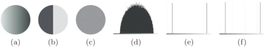
Thus, to take into account the spatial consistency, total variation minimiza-tion of the albedo seems to be a more consistent choice than entropy mini-mization, which cannot choose between different configurations having the same histogram of albedo, as shown in Fig.1. As the albedo is linked to the vector field M by ρ = ||M ||, and as the GBR transformation G with parameters µ, ν and λ transforms M into M G(µ, ν, λ), we could look for a GBR transformation which minimizes T V (||M G(µ, ν, λ)||), i.e estimate the three parameters (µ, ν, λ) such that:
(bµ,bν, bλ) = argmin
(µ,ν,λ)
(a) (b) (c) (d) (e) (f)
Fig. 1: Three different albedo configurations and the corresponding histograms: (a) has a huge entropy value, cf. histogram (d); (b) and (c) have the same small entropy, cf. histograms (e) and (f), but the spatial distributions of the albedo are very different. Total variation would tend to favor distributions like (b).
But we can do even better: it seems reasonable to also ensure that the unit normal field N should vary few inside zones. Thus one can consider minimizing both the total variation of the albedo and the total variation of the field. As they are simply linked by M = ρN , we can try to estimate this GBR transformation:
(µ,b bν, bλ) = argmin
(µ,ν,λ)
T V(M G(µ, ν, λ)) (9)
Doing so, we will favor homogeneous zones in terms of both albedo and normals, but still allowing edges, so that we do not prevent edges in the albedo map or in the normal field (which would lead to smooth shapes).
The following calculation gives a hint of it, and shows that minimizing T V(M ) is linked to minimizing simultaneously T V (ρ) and T V (N ):
kJ(M )kF = kJ(ρN )kF (10) = kNTJ(ρ) + ρJ(N )k F (11) = k (∇ρ N )⊤+ ρJ(N )kF (12) 6 k (∇ρ N )⊤kF+ kρJ(N )kF (13) = k∇ρk2+ ρ kJ(N )kF (14) 6 k∇ρk2+ kJ(N )kF (15)
The equality (14) comes on one hand from a direct calculation using the fact that N has norm 1 and on the other hand from the fact that ρ is positive. The last inequality comes from the fact that ρ ∈ [0, 1]. From this, it follows that :
T V(M ) ≤ T V (ρ) + T V (N ) (16) Note also that RR2ρkJ(N )kF is the ρ-weighted total variation of N and when
minimizing it, it allows for “relaxing” the minimization of T V (N ) where the albedo is low, i.e, where the material is dark. As it is obvious that an albedo equal to zero induces an ill-posedness in normals, this “relaxation” allows us not to consider areas which would induce errors in the reconstruction.
5
Our Model
5.1 Formal Definition
One can now rewrite the full problem of uncalibrated (Lambertian) photometric stereo as the estimation of the field M , the light matrix S and the three GBR parameters µ, ν and λ. We can write this estimation problem as the constrained regularized optimization problem of Eq.17:
( cM , bS,µ,b bν, bλ) = argmin (M,S,µ,ν,λ) P p∈ΩkIp− MpSk2 +α T V (M G(µ, ν, λ)) s.t. curl(M ) = 0 (17)
• The loss function is here the l2-norm between the data and the images
pro-duced by our estimated field and lights, which is the reprojection error. This allows a Gaussian random noise on the input data.
• The penalty function is the TV-regularization of the estimated field trans-formed by a GBR, which as we explained in the previous section will allow us to estimate the “optimal” parameters µ, ν and λ.
• The constraint is the integrability constraint, which can be rewritten as
∂ ∂y( Mx(p) Mz(p)) = ∂ ∂x( My(p)
Mz(p)) for any pixel p ∈ Ω.
• α is the weight between the loss function and the penalty function.
To solve the problem in 17 which looks very much like the Rudin-Osher-Fatemi model [23] apart from the transformation G, one could think separating the problem into two optimization problems. One of them would be a simple least-square problem, the other looks very much like a total variation based zooming problem like in [20], which could be solved by some kind of primal-dual scheme like [6]. But, although this looks really nice, our tests have shown to be quite disappointing: finding the right α is really painful as wrong choices of it will either produce an over-smoothed field or let the GBR unsolved.
We propose another approach which is actually much simpler as it does not involve such a hyper-parameter. We replace 17 by the following pair of minimization problems, which must be solved sequentially:
( cM , bS) = argmin (M,S) P p∈ΩkIp− MpSk2 s.t. curl(M ) = 0 (µ,b bν, bλ) = argmin (µ,ν,λ) T V( cM G(µ, ν, λ)) (18)
After the optimization process, the resulting field is given by M = cM G(µ,b bν, bλ), and the resulting light matrix by S = G−1(bµ,bν, bλ) bS.
5.2 The Full 3-step Solution
To solve the optimization problem in18, we adopt the common method used by (among others) Alldrin et al. in [3] or by Favaro and Papadhimitri in [10]:
1. First find a pair (M, S) which minimizes the loss function. As this is a l2
-norm, this can be achieved using SVD as proposed by Hayakawa in [14] (see Sec. 3). This gives U ∈ R|Ω|×3, W ∈ R3×3 and V ∈ Rm×3, so that
I ≈ U W VT. In the end we get M = U PT and S = QVT, where P and Q
are unknown 3 × 3 matrices holding PTQ= W .
2. Then restrict P by integrability. In some sense we “project” M on the space of integrable fields to force the estimated field to respect the constraint. This is done identifying 6 out of the 9 cofactors of P (i.e. the coefficients of P−1),
as explained by Yuille and Snow in [30]. We fix the remaining 3 cofactors to empirical values, assuming they will be “corrected” in the next step. We know that this linear transformation will not affect the loss function, so up to this point we have solved the first part of 18.
3. Finally solve for the GBR, to estimate the three parameters µ, ν and λ that minimize T V ( cM G(µ, ν, λ)), where cM = U PT. This is achieved using some
standard convex optimization method. In our tests we used the “fminunc” function of Matlab which is basically a variant of a Gauss-Newton algorithm, specifying a literal expression for the gradient which can be easily obtained by differentiating the penalty function with respect to each parameter. As the GBR is a linear transformation, the loss function will not be affected, and we know a GBR maintains integrability, so the constraint is not violated. Then both the loss function and the penalty function are minimized, and the constraint is respected. Thus, we can finally compute cM = U PTG(
b µ,bν, bλ) and bS = G−1(
b
µ,bν, bλ)P−TW VT which are our field and light solutions.
5.3 Initialization Issues
The total variation being convex but not strictly convex, the starting point for the gradient descent has to be carefully chosen. In the step 3 of the al-gorithm above, we initialize the optimization process with the solution to the l2-regularized problem with λ = 1:
(µb0,bν0) = argmin (µ,ν)∈R×R X p∈Ω kJ(M (p)G(µ, ν, 1))k2 F (19)
which, writing down the Euler-Lagrange equations, gives:
b µ0= X p∈Ω ∂Mx ∂x (p) ∂Mz ∂x (p) + ∂Mx ∂y (p) ∂Mz ∂y (p) (∂Mz ∂x (p)) 2+ (∂Mz ∂y (p)) 2 bν0= X p∈Ω ∂My ∂x (p) ∂Mz ∂x (p) + ∂My ∂y (p) ∂Mz ∂y (p) (∂Mz ∂x (p)) 2+ (∂Mz ∂y (p)) 2 (20)
which depends only on the already computed M = U PT field, and thus can be
Problem 9 can then be solved efficiently by a few Gauss-Newton iterations (less than 10 iterations in every test we ran).
Note that we do not solve this TV problem the usual way: one would expect to use some algorithm like Chambolle’s [6] to recover the whole field. Here we do not need doing so because we assume we already have a field M , and we only want to estimate the 3 parameters of the GBR which transform this field. It is a much easier 3-parameters problem which can be solved by standard optimization methods.
6
Experiments
In this section, we give some results obtained with the method described before. As dealing with outliers like shadows or highlights is not our point in this paper, we just skip the preprocessing part. We use preprocessed data that can be found on Papadhimitri’s and Alldrin’s homepages, five set of images from the Yale Dataface B [13] and synthetic images generated with the Lambertian model.
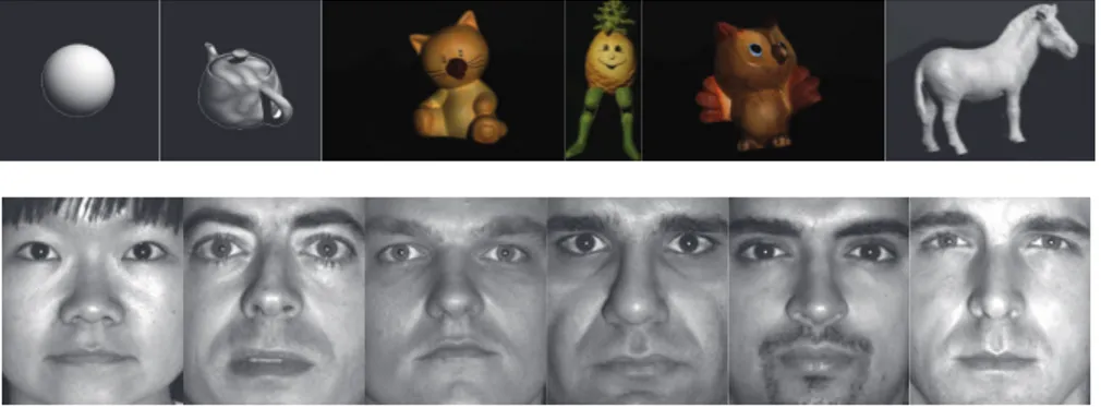
One image of each set is presented in Fig.2. Note that the Sphere and Teapot dataset contain 8 images, Cat, Owl and Horse datasets contain 12 images, the Doll dataset contains 15 images, and the Faces datasets contain 21 images each.
Fig. 2: One image of each dataset used for validating our method.
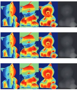
We compare in Fig. 3 the recovered normals and depth maps on the Cat dataset to both a “ground truth” which is the result from calibrated photometric stereo, and to the results from [10]. Note how close the three results are. Some rendered images can be found in Fig.4 and Fig.5.
We also show in Table1a comparison of the angular errors (expressed in de-grees) between normal fields estimated by uncalibrated photometric stereo tech-niques and by calibrated photometric stereo. We chose to compare our method to the Diffuse-Maxima method [10] which seems to be the most efficient known method, and to Minimum-Entropy [3] because our approach can be seen as an
extension of this one. Our method appears to be as good as the most state-of-the-art uncalibrated photometric stereo method for Lambertian models, and slightly faster, even though the tests were made without any special care in the optimization task, so the method could still be greatly accelerated.
Fig. 3: Normal and depth comparison. From left to right: first, second, and third components of the normal, and height map. First row: calibrated photometric stereo. Second row: diffuse maxima [10]. Third row: our method.
(a) (b) (c) (d)
Fig. 4: Cat reconstruction: (a,c) calibrated PS (frontal and lateral views); (b,d) our method (frontal and lateral views).
(a) (b) (c) (d) (e) (f)
Fig. 5: Faces reconstructions (lateral views), with estimated albedo mapped as texture.
Dataset Sphere Teapot Cat Doll Owl Horse ME 5.64(19.22 s) 24.01 (27.83 s) 13.91 (20.82s) 27.67 (15.18 s) 16.16 (25.15 s) 11.10 (15.80 s) DM 6.84 (1.59 s) 23.94 (2.09 s) 5.37 (1.22 s) 12.15 (1.11 s) 6.63 (1.07 s) 4.80(1.62 s) TV 6.29 (1.40 s) 16.48 (1.41 s) 5.26 (0.67 s) 11.90 (0.69 s) 7.06 (0.76 s) 5.53 (0.67 s) Dataset YaleB05 P00 YaleB06 P00 YaleB07 P00 YaleB08 P00 YaleB09 P00 YaleB10 P00 ME 9.44 (14.90 s) 18.00 (14.57 s) 12.63 (14.62 s) 19.61 (14.79 s) 17.10 (14.45 s) 9.22 (13.72 s) DM 6.90(2.07 s) 11.46 (1.98 s) 8.59 (1.84 s) 11.49 (1.29 s) 13.09 (1.11 s) 10.21 (3.63 s) TV 13.33 (0.59 s) 7.94 (0.50 s) 10.25 (0.55 s) 8.80 (0.52 s) 7.94(0.51 s) 8.34 (0.56 s)
Table 1: Performance comparison of TV with the Minimum-Entropy method (ME) [3] and with the Diffuse-Maxima (DM) method [10]. We give the mean angular error (in degrees) of the estimated normal field and the CPU time.
7
Conclusion
In this paper, we presented a novel approach to the resolution of the generalized bas-relief ambiguity, introducing the total variation of the estimated field. We showed how this approach could produce a new model for uncalibrated photo-metric stereo and gave a very simple and efficient algorithm for finding a solu-tion to this problem. Unlike most attempts to solve this issue, our method does not rely on any property of the scene except its Lambertian reflectance, so the method should work for any Lambertian dataset. For a real world application though, it would be necessary to make a preprocessing step on the data in order to remove the outliers.
We also compared the solution given by our algorithm to the most efficient known method, and the results show that our method performs as good as it. The key point of it is the optimization step of the algorithm, which could be greatly improved in order to get a really fast solver. This would open the doors to some real-time reconstruction in the wild using photometric stereo, and could be useful for many applications like augmented reality.
References
1. A. Abrams, C. Hawley, and R. Pless. Heliometric Stereo: Shape from Sun Position. In ECCV, LNCS 7573, pages 357–370, 2012. 2
2. J. Ackermann, F. Langguth, S. Fuhrmann, and M. Goesele. Photometric Stereo for Outdoor Webcams. In CVPR, pages 262–269, 2012. 2
3. N. G. Alldrin, S. P. Mallick, and D. J. Kriegman. Resolving the Generalized Bas-relief Ambiguity by Entropy Minimization. In CVPR, 2007. 1,3,5,8,9,11
4. P. N. Belhumeur, D. J. Kriegman, and A. L. Yuille. The Bas-Relief Ambiguity.
IJCV, 35(1):33–44, 1999. 1,3
5. X. Bresson and T. Chan. Fast Dual Minimization of the Vectorial Total Variation Norm and Applications to Color Image Processing. Inverse Problems and Imaging, 2(4):455–484, 2008. 5
6. A. Chambolle. An Algorithm for Total Variation Minimization and Applications.
7. M. K. Chandraker, F. Kahl, and D. J. Kriegman. Reflections on the Generalized Bas-Relief Ambiguity. In CVPR (vol. I), pages 788–795, 2005. 3
8. O. Drbohlav and M. Chantler. Can Two Specular Pixels Calibrate Photometric Stereo? In ICCV (vol. II), pages 1850–1857, 2005. 1,3
9. J.-D. Durou, J.-F. Aujol, and F. Courteille. Integration of a Normal Field in the Presence of Discontinuities. In EMMCVPR, LNCS 5681, pages 261–273, 2009. 2
10. P. Favaro and T. Papadhimitri. A Closed-Form Solution to Uncalibrated Photo-metric Stereo via Diffuse Maxima. In CVPR, pages 821–828, 2012. 1,3,8,9,10,
11
11. R. T. Frankot and R. Chellappa. A Method for Enforcing Integrability in Shape from Shading Algorithms. PAMI, 10(4):439–451, 1988. 2
12. A. S. Georghiades. Incorporating the Torrance and Sparrow model of reflectance in uncalibrated photometric stereo. In ICCV (vol. II), pages 816–823, 2003. 3
13. A. S. Georghiades, D. J. Kriegman, and P. N. Belhumeur. From Few to Many: Illumination Cone Models for Face Recognition under Variable Lighting and Pose.
PAMI, 23(6):643–660, 2001. 9
14. H. Hayakawa. Photometric stereo under a light-source with arbitrary motion.
JOSA A, 11(11):3079–3089, 1994. 1,2,4,8
15. C. Hern´andez, G. Vogiatzis, G. J. Brostow, B. Stenger, and R. Cipolla. Multiview Photometric Stereo. PAMI, 30(3):548–554, 2008. 2
16. A. Hertzmann and S. M. Seitz. Example-Based Photometric Stereo: Shape Recon-struction with General, Varying BRDFs. PAMI, 27(8):1254–1264, 2005. 3
17. B. K. P. Horn. Obtaining Shape from Shading Information. In Shape from Shading, pages 123–171. MIT Press, 1989. 2
18. B. K. P. Horn. Height and Gradient from Shading. IJCV, 5(1):37–75, 1990. 2
19. Z. Lin, M. Chen, and Y. Ma. The Augmented Lagrange Multiplier Method for Exact Recovery of Corrupted Low-rank Matrices. Tech. Rep. UILU-ENG-09-2215, UIUC, 2009. 3
20. F. Malgouyres and F. Guichard. Edge Direction Preserving Image Zooming: A Mathematical and Numerical Analysis. SIAM Num. Anal., 39(1):1–37, 2001. 7
21. M. Nikolova. Minimizers of Cost-functions Involving Non-smooth Data-fidelity Terms. Application to the Processing of Outliers. SIAM Num. Anal., 40(3):965– 994, 2002. 5
22. R. Onn and A. M. Bruckstein. Integrability Disambiguates Surface Recovery in Two-Image Photometric Stereo. IJCV, 5(1):105–113, 1990. 2
23. L. I. Rudin, S. Osher, and E. Fatemi. Nonlinear Total Variation Based Noise Removal Algorithms. Physica D: Nonlin. Phen., 60(1–4):259–268, 1992. 1,7
24. B. Shi, Y. Matsushita, Y. Wei, C. Xu, and P. Tan. Self-calibrating Photometric Stereo. In CVPR, 2010. 3
25. D. Strong and T. Chan. Edge-preserving and Scale-dependent Properties of Total Variation Regularization. Inv. Probl., 19(6):S165–S187, 2003. 2
26. K. Sunkavalli, T. Zickler, and H. Pfister. Visibility Subspaces: Uncalibrated Pho-tometric Stereo with Shadows. In ECCV, LNCS 6312, pages 251–264, 2010. 3
27. P. Tan, S. P. Mallick, L. Quan, D. J. Kriegman, and T. Zickler. Isotropy, reciprocity and the generalized bas-relief ambiguity. In CVPR, 2007. 3
28. R. J. Woodham. Photometric Method for Determining Surface Orientation from Multiple Images. Opt. Engin., 19(1):139–144, 1980. 1,2
29. L. Wu, A. Ganesh, B. Shi, Y. Matsushita, Y. Wang, and Y. Ma. Robust Photo-metric Stereo via Low-Rank Matrix Completion and Recovery. In ACCV, LNCS
6494, pages 703–717, 2010. 3
30. A. L. Yuille and D. Snow. Shape and Albedo from Multiple Images using Integra-bility. In CVPR, pages 158–164, 1997. 1,3,4,8
![Table 1: Performance comparison of TV with the Minimum-Entropy method (ME) [3] and with the Diffuse-Maxima (DM) method [10]](https://thumb-eu.123doks.com/thumbv2/123doknet/3586728.105238/12.892.202.725.175.253/table-performance-comparison-minimum-entropy-method-diffuse-maxima.webp)
