On the Alternate Direction Implicit (ADI) Method for Solving Heat Transfer in Composite Stamping

(1)

HAL Id: hal-03190763

https://hal.archives-ouvertes.fr/hal-03190763

Submitted on 6 Apr 2021

HAL is a multi-disciplinary open access

archive for the deposit and dissemination of

sci-entific research documents, whether they are

pub-lished or not. The documents may come from

teaching and research institutions in France or

abroad, or from public or private research centers.

L’archive ouverte pluridisciplinaire HAL, est

destinée au dépôt et à la diffusion de documents

scientifiques de niveau recherche, publiés ou non,

émanant des établissements d’enseignement et de

recherche français ou étrangers, des laboratoires

publics ou privés.

Solving Heat Transfer in Composite Stamping

Arthur Lévy, Duc Anh Hoang, Steven Le Corre

To cite this version:

Arthur Lévy, Duc Anh Hoang, Steven Le Corre. On the Alternate Direction Implicit (ADI) Method

for Solving Heat Transfer in Composite Stamping. Materials Sciences and Applications, Scientific

Research, 2017, 08 (01), pp.37-63. �10.4236/msa.2017.81004�. �hal-03190763�

(2)

http://www.scirp.org/journal/msa ISSN Online: 2153-1188

ISSN Print: 2153-117X

On the Alternate Direction Implicit (ADI)

Method for Solving Heat Transfer in

Composite Stamping

Arthur Levy

1

_{, Duc Anh Hoang}

1,2

_{, Steven Le Corre}

1

1_{Laboratoire de Thermique et Energie de Nantes, La Chantrerie, Rue Christian Pauc, Nantes, France} 2_{IRT Jules Verne, Chemin du Chaffault, Bouguenais, France}

Email: arthur.levy@univ-nantes.fr, duc-anh.hoang@irt-jules-verne.fr, steven.le-corre@univ-nantes.fr

Abstract

Thermostamping of thermoplastic matrix composites is a process where a preheated blank is rapidly shaped in a cold matching mould. Predictive mod-elling of the main physical phenomena occurring in this process requires an accurate prediction of the temperature field. In this paper, a numerical me-thod is proposed to simulate this heat transfer. The initial three-dimensional heat equation is handled using an additive decomposition, a thin shell as-sumption, and an operator splitting strategy. An adapted resolution algorithm is then presented. It results in an alternate direction implicit decomposition: the problem is solved successively as a 2D surface problem and several one- dimensional through thickness problems. The strategy was fully validated versus a 3D calculation on a simple test case and the proposed strategy is shown to enable a tremendous calculation speed up. The limits of applicability of this method are investigated with two parametric studies, one on the thick-ness to width ratio and the other one on the effect of curvature. These condi-tions are usually fulfilled in industrial cases. Finally, even though the method was developed under linear assumption (constant material properties), the strategy validity is extended to multiply, temperature dependant (nonlinear) case using an industrial test case. Because of the standard methods involved, the proposed ADI method can readily be implemented in existing software.

Keywords

Thin Plates, Alternate Direction Implicit, Shell Theory, Operator Splitting, In-Plane Variations

1. Introduction

1.1. Context

Thermoplastic composites offer new possibilities for the industry. Large struc-

How to cite this paper: Author 1, Author 2 and Author 3 (2017) Paper Title. Mate-rials Sciences and Applications, 8, *-*.

http://dx.doi.org/10.4236/***.2017.*****

Received: **** **, *** Accepted: **** **, *** Published: **** **, ***

http://creativecommons.org/licenses/by/4.0/

(3)

tures can be processed rapidly and more cost-effectively than when thermoset composites are used, since the latter need to undergo lengthy curing reactions. The ability to fuse thermoplastic resins gives new perspectives for forming processes.

The thermostamping process is derived from the metallic materials industry. Forming occurs in two steps. In a first step, a semi-finished thermoplastic flat laminate, called the blank, is heated above the processing temperature of the matrix, usually using infra-red lamps. In the second step, this hot blank is quickly transferred to a cooled mould where it is stamped and given its final shape [1] [2]. The heating and cooling steps are therefore separated. This results in an high production rate that makes this process very attractive for the industry.

Even though metal stamping has been the subject of extensive research work in the past decades (see for instance the review by Karbasian and Tekkaya [3]), thermostamping of composite materials adds a new level of complexity for two resons. Indeed, the mechanical deformation and heat transfer occurring in the blanks may result in a complex and unexpected behaviour, especially when dealing with textile composite laminates. Nonetheless, accurate modelling and prediction of the main physical phenomena involved are prerequisite for an efficient process optimization.

1.2. Heat Transfer in Composite Stamping

It is well established that the temperature evolution is of major importance in this forming process. Keeping this in mind, de Luca et al. [4] or Cao et al. [5] proposed to take the blank temperature into account in the mechanical predictions of thermostamping process. Cao et al. [5] considered only two possible state: a high temperature state before the blank comes in contact with the mould, and a low temperature state after contact occurs. Based on previous work by Pickett et al. [6], de Luca et al. [4] propose a modelling of the through thickness heat transfer using finite volume but are only able to predict the average temeprature per ply in the case of a composite laminate. In thermostamping process thought, and especially during the stamping step, because of the thermal shock between the cold mould and the hot blank, high through-thickness temperature gradients may arise. The models by these authors, based on rough approximations of the through thickness temperature profiles, cannot accurately describe these high through-thickness variations.

A finer through thickness temperature distribution description was proposed by Thomann et al. [7] using a finite difference method. Nonetheless they neglected the in-plane effects and thus considered only unidirectional through- thickness heat transfer. On the contrary, in real industrial processes, in-plane diffusion and 3D effects cannot be neglected, especially when boundary condition sharply evolve (in the vicinity of cavity edges) or in case of curved geometries. In the present paper, a fine description of the through thickness temperature profile, in conjunction with the in-plane transfer is proposed.

(4)

Furthermore, the proposed model is designed to be easily implemented in any existing industrial code (such as Plasfib [8], Aniform [9] or PAM-Form [4]). The heat transfer problem should then be solved within acceptable computational times. With this aim, the full three-dimensional heat transfer problem cannot be solved using standard methods. Instead, a model reduction is necessary.

Considering the composite blank as a thin shell, it is natural to decompose the 3D temperature solution into a shape function and an in-plane temperature. As suggested by Saetta and Rega [10], it writes

{

temperature3D

} {

= shape

} {

× temperature .

}

(1)

With this decomposition, the accuracy of through thickness description depends on the type of shape functions chosen. Within this framework, some authors suggested to construct new 3D shell finite elements that integrate this through thickness heat transfer effects [11] [12] [13] [14]. Nonetheless, using one single shell element in the thickness highly restricts the possible through- thickness temperature profile description. Even with the parabolic shape pre- supposed by Alves Do Carmo and Rocha De Faria [15] or the higher order interpolation proposed by Surana and Abusaleh [13], sharp profiles that arise in case of the thermal shocks that occur in thermostamping, will not be accurately described.

Adopting a fine through-thickness discretization therefore seems a more flexible approach, though potentially time-consuming. In this idea, Bognet et al.

[16] wrote the above decomposition as a sum of separated modes

{

temperature3

}

(

{

shape

} {

_i temperature

}

_i

)

i

D =

∑

×

where the shape functions, themselves, are described with a fine discretization involving hundreds of degrees of freedom. In this framework, Bognet et al.

considered a series of multiplicative shape functions, where each mode i is the product of an out-of-plane function by an in-plane function. The out-of-plane function is therefore identical for all the points of the shell. Using this in-plane/ out-of-plane separation, a solving strategy using the proper generalized decomposition (PGD) was proposed for the elastic problem on a shell like domain. More recently, the [17] the method has been extended to nonlinear thermal problems. Though possibly efficient in some cases, such a resolution strategy in the environments of existing codes might be challenging. In particular, dealing with space varying boundary conditions and material non-linearity requires complicated developments and a probably a high number of modes.

1.3. Alternate Direction Implicit (ADI) Decomposition

In this paper, starting from a very general approximation framework as given by Equation (1), we propose a reduced numerical scheme, adapted to thin composite shells, that preserves the three-dimensional nature of the heat transfer problem but takes advantage of the good physical separation between in-plane and out-of-plane phenomena, even in case of anisotropic thermal properties.

(5)

The present method is based on an operator splitting technique that enables to simplify a time evolution problem implying several spatial dimensions. The general framework of operator splitting techniques always considers an incremental iterative time integration strategy. Over 50 years ago, Douglas [18] and Douglas and Rachford [19] suggested to treat separately, within one time step, the different spatial directions. This led to the so called locally one-dimensional methods [20] or alternate direction implicit (ADI) methods. Then, numerous extension were proposed to reduce the error of the splitting strategy, and to validate the convergence and stability of the schemes, in linear and nonlinear cases [21] [22] [23] [24].

Following these ideas, the present paper proposes an operator splitting strategy adapted to the composite shell problems to solve the reduced heat transfer model. In fine, this results in two separated problems. A solving algorithm and numerical implementation is then proposed. The approach is validated on a flat plate test case, and its limits are determined with parametric studies. The method validity is extended to nonlinear cases with an industrial application.

2. Methods

2.1. Initial Heat Transfer Problem

2.1.1. Domain

The heat transfer problem is solved in the domain Ω representing a composite laminate blank. It is considered to be an arbitrary curved thin shell, where the local positions are located via a curvilinear parallel coordinate system

(

p q z, ,

)

.

A local frame

(

e e e_p, _q, _z

)

can be attached to each point. Coordinate z enables the location of points along the thickness direction, that is to say along ez, the

normal vector to the shell mid-plane (see Figure 1). In this domain the composite material is considered to be a continuous medium with effective homogeneous properties.

2.1.2. Heat Equation

In the considered heat transfer problem, the conduction is assumed to be governed by an anisotropic Fourier law where the local heat flux q is written

as:

T

= − ∇

q K (2)

where K is the thermal conductivity tensor, T the temperature field and ∇ ⋅

the spatial derivative operator. In the present work, it is assumed that the through thickness direction z is a principal direction of the thermal conductivity. This is a classical assumption in the case of standard composite laminates [10] [25]. Thus, in the

(

e e e_p, _q, _z

)

basis, it writes

( )

[ ] [ ]

[ ]

₍₍ _, ₎_, ₎ , , 0 0 0 , 0 0 0 pp pq qp qq z _{p q z} z p q z K K K K K K       =_ _ _{= } _       s K K (3)

(6)

Figure 1. Shell like domain Ω on which the heat transfer problem is solved. ez de-

notes the out of plane direction and h the thickness of the laminate. A typical in-plane dimension is L1 m.

s

K being the in-plane thermal conductivity tensor and Kz the through

thickness thermal conductivity. Note that this hypothesis fails in the case of complex 3D architectured composites. Defining the in-plane surface gradient

s

∇ ⋅_{, Equation (2) can be separated into a through thickness and an in-plane}

fluxes: . s s z z T T K z ∂ = − ∇ − ∂ q K e (4) In the case of a flat shell Ω , the coordinate system

(

p q z, ,

)

is the natural

cartesian coordinate system

(

X Y Z, ,

)

, and ∇ • = ∂ • ∂ ∂ • ∂s

(

X, Y

)

T. In the

more complex case of an arbitrary curved shell Ω , the reader should refer to Appendix for a proper definition of the surface gradient ∇ ⋅s . This demons-

tration shows that in the case of a thin shell with small curvature, the operator

s

∇ ⋅_{does not depend on the through thickness position} z.

Using this separation, without internal heat source in the domain Ω , the energy balance typically writes

(

)

p s s s z T T c T K t z z ρ ∂ = ∇ ⋅ ∇ + ∂ _ ∂ _ ∂ K ∂  ∂  (5)

ρ

being the density of the composite material and cp its specific heat. Once

again, for a flat shell, the surface divergence ∇ ⋅• = ∂ • ∂ + ∂ • ∂s X Y , but for

curved shell, it is defined in Appendix and it is constant through thickness.

2.1.3. Boundary and Initial Conditions

The domain Ω is bounded by the boundaries Γlat, Γsup and Γinf, as defined

in Figure 1. For the sake of simplicity, the lateral boundaries are considered insulated:

lat

0 on

T

∇ ⋅ =n Γ (6)

n being the outward normal to each surface. Conversely, in order to accurately model temperature history imposed on the upper and lower boundaries

sup

(7)

(

)

(

)

sup

sup imp sup

inf

inf imp inf

on . on z z T K h T T z T K h T T z ∂  ⋅ = − = − Γ  ∂  _∂  ⋅ = = − Γ  ∂  q n q n (7) where sup imp

T (respectively Timpinf) is the temperature imposed on the upper (re-

spectively lower) boundary and hsup (respectively hinf) is the heat exchange

coefficient. This mixed boundary condition modelling can account for non ideal contact with the mould [11] [12]. In its limit form, it is also suited to model both Dirichlet or Neumann boundary conditions. Note that the development proposed hereunder could seemlessly be conducted with any type of boundary conditions (temperature imposed, heat flux, radiating surface...).

The initial temperature field, assumed given, is defined as:

(

0

)

init

(

, ,

)

.

T t= =T p q z (8)

2.2. Alternate Direction Implicit (ADI) Model

This section presents a reduction of the heat transfer problem defined above. The reduced boundary value problem is obtained thanks to an intuitive decomposition of the temperature field and a thin shell assumption. An implementation strategy is then proposed to numerically solve this problem. Here, for the sake of clarity, the heat transfer problem is assumed linear (the material properties

ρ

, cp and K do not depend on the temperature T ). The extension

to nonlinear case will be discussed with a test case in Section 3.3.

2.2.1. Additive Decomposition

The first step in the proposed model reduction is to seek the solution T of the system of Equations (5) to (8) as a sum of a through thickness averaged field and of a fluctuation field:

(

, , ,

)

_z

(

, ,

)

(

, , ,

)

T x y z t = T x y t + T x y z t (9)

where the operator

2

1 • h • d

z =_h

∫

−h z (10)

is the through thickness average, h being the local shell thickness. It is obvious that using this additive decomposition, the average field T z does not depend

on the z-coordinate whereas the fluctuation field T has a zero thickness average. This decomposition is intuitive and does not necessitate any assumption. Substituting this decomposition (9) in the heat Equation (5), considering constant material properties, and noting that T z and the operator ∇s do

not depend on the z-coordinate gives:

(

)

(

)

. z p p s s s z s s s z T _T _T c c T T K t t z z ρ ∂_∂ +ρ ∂_∂ = ∇ ⋅ ∇ + ∇ ⋅ ∇ +_∂∂  ∂_∂     _  K K (11)

Applying the average operator ⋅z on both hands of this equation leads to

(

)

2 2 1 . h z p s s s z z h T T c T K t h z ρ − ∂  ∂  = ∇ ⋅ ∇ _{+ } _ ∂ _ ∂ _  K (12)

(8)

By defining the upper and lower inward boundary fluxes

(

)

(

)

sup z 2 inf z 2 , T T K z h K z h z z ∂ ∂ Φ = = Φ = − = − ∂ ∂   (13) Equation (12) writes:

(

)

sup inf z p s s s z T c T t h ρ ∂ = ∇ ⋅ ∇ +Φ + Φ ∂ K (14)

which is the average field heat equation. It rules the in-plane mean field temperature evolution. Subtracting this mean heat equation from Equation (11) results in the fluctuating heat equation:

(

)

sup inf p s s s z T T c T K t z z h ρ ∂ = ∇ ⋅ ∇ + ∂ _ ∂ _−Φ + Φ ∂ ∂ _ ∂ _  _  K (15)

which rules the through thickness temperature fluctuation.

Assuming a thin plate for which hL, the so called aspect ratio for conduction: 2 1 s z K h A K L   = _{ }    (16) and the dimensional analysis safely leads to

(

)

. s s s z T T K z z   ∂ ∂ ∇ ⋅ ∇ _ _ ∂ _ ∂ _    K (17) Equation (15) then reduces to the fluctuating field heat equation:

sup inf . p z T T c K t z z h ρ ∂ = ∂ _ ∂ _−Φ + Φ ∂ ∂ _ ∂ _   (18) Equations (14) and (18) achieve a decomposition of the initial heat Equation (5) in the average and fluctuating contributions. Nonetheless, without further assumptions, these two equations are strongly coupled through the source terms

(

Φ + Φsup inf

)

h.

Reduced model. Summing Equations (14) and (18), and adding the term 0 z z T K z z  ∂  ∂ =     ∂ _ ∂ _ , gives

(

)

. p s s s z z T T c T K t z z ρ ∂ = ∇ ⋅ ∇ + ∂ _ ∂ _ ∂ K ∂  ∂  (19)

This equation, along with boundary and initial conditions (6), (7) and (8) defines the reduced boundary value problem ( P ). In the bulk Equation (19), the first spatial differential operator of the right hand side acts on the average parts of the temperature field T z only. The solving of this reduced boundary value

problem is therefore not straightforward. In the next section, a numerical method is proposed to solve this original model. It will also confirm its well-posedness.

2.2.2. Operator Splitting

(9)

solved in the framework of a standard incremental iterative time integration scheme. At a given time tn, the solution Tn

(

x y z, ,

)

is supposed to be known.

Then, the solution Tn+1

(

x y z, ,

)

of the reduced boundary value problem

defined above is searched at next time step tn+1= +tn dt.

Any conventional time integration scheme, such as for example explicit or implicit schemes, can be used to determined Tn+1

(

x y z, ,

)

in terms of Tn

(

x y z, ,

)

,

so that the developments detailed hereunder will easily be implemented in such software environment.

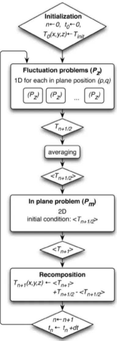
Operator splitting. To solve Equation (19), an operator splitting method is used. This numerical method enables to solve evolution equations that involve a sum of differential operators (see for example [20]). Adopting the splitting initially suggested by Douglas [18] and later called locally one-dimensional (LOD) method (see for instance [26] and references therein), the two differential operators in the right hand side of Equation (19) are considered separately. Note that in this linear case, the proposed splitting does not introduce additional numerical error beside the time integration error [20]. As illustrated in Figure 2, a so-called fractional time step method is adopted, where two problems are solved successively, each one containing one of the operators:

• Step 1: solve the following 1D boundary value problem called (Pz) over one

full time step dt

(

)

(

)

sup

sup imp sup

inf

inf imp inf

on on at p z z z n n T T c K t z z T K h T T z T K h T T z T T t t ρ  ∂ ₌ ∂  ∂     _∂ _∂ _ _∂ _   ∂ − = − Γ   ∂  _∂  = − Γ ∂   = =  (20)

Figure 2. Operator splitting strategy. Instead of solving the full evolution equation on one time step, each differential operator is addressed successively. The initial condition of the second step is the field obtained at the end of the first step.

(10)

gives the intermediate result Tn+1 2

(

x y z, ,

)

at the end of the time step

1 d

n n

t + = +t t.

• Step 2: solve the 2D boundary value problem over one full time step dt

(

)

lat 1 2 0 on at p s s s z s n n T c T t T T T t t ρ + ∂  _{= ∇ ⋅} _∇  _∂  ∇ ⋅ = Γ   = =   K n (21)

where the initial condition Tn+1 2 is the value of the field computed in step 1.

The solution of this second step at the end of the time step (tn+1= +tn dt) is

identified to Tn+1.

Whereas the system (Pz) defined in step 1 is a well posed unidimensional

partial differential equation, it is somewhat disturbing that both T and T z

appear in the problem (21) defined in step 2.

ADI model. To ensure the well-posedness of this step 2, the additive decomposition (9) is again substituted in system (21). Applying the average operator

z

⋅ gives the in-plane boundary value problem (Pm)

(

)

lat 1 2 . 0 on at . z p s s s z s z n n z z T c T t T T T t t ρ +  ∂ = ∇ ⋅ ∇  ∂ _∇ ₌ _Γ   ₌ ₌   K n (22)

Finally, subtracting (22) from (21) results in

(

)

1 2 1 2 0 p n n n _z T c t T t t T T ρ + +  ∂ =  _∂   ₌ ₌ ₋    (23)

which admits the trivial constant solution:

1 2 1 2 .

n n _z

T=T+ − T+ (24)

Therefore, the fluctuating part T of this second step is simply the fluctuating part of Tn+1 2 computed in the first step. In other terms, this second step does

not introduce any additional out-of-plane fluctuation to the solution.

2.3. Numerical Algorithm

To ensure spatial numerical integration of this problems, a spatial discretization has to be adopted. Within the defined shell like domain Ω a natural extruded discretization is assumed. Thus, and without loss of generality, for each in-plane discrete position

(

p qi, i

)

amongst Ns nodes, there is Nz out of plane nodes.

The dimension of the 3D discretized field is then Ns×Nz.

Resolution scheme.

Following the above additive decomposition and operator splitting strategy,

(

)

(

)

(

)

(

)

( ) 1 1 1 2 1 2 , , 1 , , , , , , . n n z n n z T_n p q z T₊ p q z T₊ p q T₊ p q z T₊ p q + = + −   (25)

(11)

In this sum,

• Tn+1 2 is obtained by solving the fluctuation 1D boundary value problem

(Pz) (Equation (20)). This problem is parametrized by the in-plane position

(

p q,

)

through the dependency of the thickness h and boundary conditions

sup

h , h_inf, sup imp

T and T_impinf. Thus, the problem (Pz) has to be solved Ns times.

Nonetheless each resolution has the complexity of a 1D boundary value problem. Furthermore, each resolution is independent, and can be solved in a parallel manner as illustrated in Figure 3.

• Tn+1 2 _z is obtained as a post-processing by averaging the above Tn+1 2

field through thickness.

• Tn+1 z is obtained by solving one single in plane 2D boundary value

problem (Pm) (Equation (22)) using the 2D field Tn+1 2 _z as an initial condi-

tion. At the end of time step dt, it gives the field Tn+1 z.

Expected computational speed up. A conventional in plane discretization of an industrial geometry would typically result in Ns ∼200 200× =40000 nodes.

Figure 3. Resolution strategy. At each time step, the solution is obtained with two successive steps: solving a set of Ns fluctuation problems (Pz) and solving one single

(12)

Additionally, because of the high through thickness temperature gradients associated with thermal shocks that occur in thermo-stamping, a fine through thickness discretization is required, for instance Nz∼50. In this case, the

number of degree of freedom reaches 6

2 10

s z

N ×N ∼ × .

Solving the initial 3D heat transfer problem defined in Section 2.1 using standard methods would result in solving a transient problem with 6

2 10 ∼ ×

degrees of freedom and a three-dimensional complexity. It would quickly result in unrealistic computational costs. Moreover, in the case of a thin shell domain, the proposed mesh, involving Ns in plane nodes and Nz through thickness

nodes, would result in anisotropic mesh that may lead to numerical errors. On the contrary, in the proposed resolution strategy, at each time step, Ns

independent 1D boundary value problem (Pz) with Nz degrees of freedom

can be solved in parallel, followed by one single 2D boundary value problem (Pm)

with Ns degrees of freedom. This strategy should result in a greatly reduced

computational cost with a preserved accuracy, which opens the way for integrat- ing such approach as sub-routine in industrial simulation tools. Moreover, the in-plane and out-of-plane mesh sizes appear in two different problems and thus saves from complicated anisotropic meshing techniques.

Asynchronous time integration. Because of the thin plate assumption where hL, the ratio between characteristic in-plane diffusion time tp and charac-

teristic through thickness diffusion time tz writes 2 . s z p z t h A t K L   = = _{ }   K

A being a dimensionless parameter characteristic of the so-called conduction

aspect ratio. In a typical industrial case, where h5 mm, L0.5 m, and 10

s Kz 

K , this ratio drops below 3

10− . Therefore, the characteristic

through thickness diffusion time is way shorter than its in-plane counterpart. This context justifies the use of an asynchronous time integration scheme, where two different time steps are used respectively for the through thickness fluctuating problem (Pz) and the in-plane problem (Pm).

In practice, the global resolution algorithm presented in Figure 3 is kept, and the global time stepping is based on the in-plane requirements (dt= 

( )

t_p ).

During each time step dt, the through-thickness problems are calculated by a

sub-integration with smaller time steps dt′ of the order dt′ = 

( )

tz .

3. Results and Discussion

In this section, first, the proposed separated model and resolution strategy is validated on a test case that largely fulfills the thin shell assumption. Then the speed up is discussed and the limits of the presented model are investigated with rougher cases (thick and curved shell).

3.1. Validation

In order to validate the proposed resolution strategy, the temperature fields obtained using the presented model are compared with the temperature fields

(13)

obtained by solving the initial three-dimensional problem, using a commercial software (COMSOL Multiphysics 5.0®_).

3.1.1. Test Conditions

A square flat plate of dimensions 2 2

0.1 0.1 m

L = × and thickness h=5 mm is

considered. The origin of the

(

x y z, ,

)

cartesian coordinate system is taken in

the centre of the plate. In such a flat plate case, the curvilinear coordinates are identified to the cartesian ones: p=x and q= y.

Material properties. In this test case, a PA66/glass fibre composite material is considered. The homogenized material properties are adapted from the litera- ture [27]. The in plane conductivity Ks is considered isotropic and all the

material properties are supposed constant and are listed in Table 1.

Boundary and initial conditions. The boundary and initial conditions are given in Table 2. The plate is supposed to be initially at uniform room temperature Tinit =20 C

 _.

A different heating condition is imposed on the upper and lower surfaces with

sup sup

imp imp

T ≠T . It is representative of the temperature imposed by a hot mould con-

tact. In order to add in-plane variability to the problem, the exchange coefficients hsup and hinf artificially depend on space position

( )

x y, through the

characteristic gaussian function

(

,

)

exp 500 2 2 2 . x y x y L χ = _− + _  

The problem is solved on the time interval t=

[

0, 20 s

]

.

3.1.2. Numerical Parameters

Numerical methods. The 1D transient boundary value problems (Pz) and

the 2D transient boundary value problem (Pm) are solved using a finite element

method with piecewise linear interpolation. An implicit (backward Euler) time integration scheme is used for all time integrations. The proposed algorithm was programmed in MATLAB®_{, which enables the parallel resolution of the (}

z

P ) problems.

Table 1. The material properties used in the test case are adapted from Faraj et al. [27].

Density ρ 3 1870 kg m⋅ − Specific heat cp 1 1 990 JK−⋅kg− In plane conductivity Kpp, Kqq 1 1 0.44 Wm−⋅K− Out of plane conductivity Kz

1 1

0.53 Wm−⋅K−

Table 2. Initial and boundary conditions used in the test case.

Initial temperature Tinit 20 C



Exchange coefficients hsup, hinf ( )

5 -2 -1

10 Wm ⋅K ×χ x y, Imposed temperature sup

imp

T 300 C

inf imp

(14)

Mesh. For the reference simulation, a 3D regular mesh made of 3600 hexa- hedron is obtained by extruding a regular in-plane 2D mesh that consists of

60 60× quadrangular elements. There are thus 30 elements in the thickness,

and in terms of nodes, Ns =3721 and Nz =31.

For the proposed separated method, the mesh consists of the same 31 nodes through the thickness for the Pz problems and of a triangular regular mesh

with the same 3721 nodes for the Pm problem.

The interpolations used in every finite element methods (3D in COMSOL, 2D in Pm and 1D in Pz) are all linear, which enables to expect for the same

precision.

Time step. Time stepping in the FEM reference simulation follows the COMSOL built-in algorithm and is forced not to exceed 0.01 s. The time

integration scheme is a standard backward difference scheme. On the contrary, a constant time step dt=0.01 s is used in the presented method. In this first test

case, the time steps for both Pz and Pm problems are the same.

The convergence of the numerical methods used was first validated on a standard one-dimensional test case by comparing the numerical solution with an analytical solution given by Jaeger [28].

3.1.3. Comparison

Figure 4 shows the in-plane temperature profiles at three different heights, at final time t=20 s. Figure 5 represents the through thickness temperature

Figure 4. Temperature profile at y= versus x for three different heights z in the 0 plate. The plot is at final time t=20 s. The reference 3D finite element solution (plain lines) is accurately recovered with the proposed methodology (markers).

(15)

Figure 5. Temperature profile at y= versus z for two different in plane positions 0

x and two different instants t. Once again, the 3D finite element solution (plain lines)

is accurately recovered with the proposed methodology (markers).

profiles in the centre and on the edge of the plate at t=0.02 s and final time 20 s

t= . The figures show a good superposition of the reference field obtained with the finite element simulation and the one obtained with the presented method. The same numerical artifact (a slight oscillation) is found with both methods in the through thickness profile at early time (t=0.02 s). This is due

to the finite element and time discretization that fail to accurately predict thermal shocks. this artifact does not influence the later time predictions (see for instance Fachinotti and Bellet [29] regarding this issue).

The maximum residual relative error

( )

(

( )

3

( )

)

sup imp init max err t T t TD t T T Ω − = − (26)

is defined, where T3D is the field computed with the 3D model in COMSOL

and T is the field computed with the presented method. At final time t=20 s,

the error err does not exceed 2.5% which represents around 6.5 C .

3.2. Efficiency and Model Limits

3.2.1. Speed up

The reference finite element simulation was computed in 10000 s on a desktop

computer (see Table 3). The solving time per time step was about 5 s. The

separated form solution was computed on the same computer in no more than

(16)

Table 3. Computational speeds, the proposed method results in a speed up of over 28 times. In case of asynchronous time stepping and parallel resolution of Pz problems,

this speed up even reaches 33 times.

Test Case CPU time per time step CPU time

COMSOL 3D 5 s 10,000 s

Proposed method, synchronous 0.178 s 356 s

m

P 0.022 s

s z

N ×P 0.145 s

Proposed method, asynchronous / 300 s

times. Using asynchronous time steps for Pm and Pz results in an additional

reduction in the total computational time. Moreover, the Pz problems are

solved in a sequential manner in this test case. Solving them in parallel results in additional speed-up.

3.2.2. Extreme Cases

The limits of the proposed resolution strategy are investigated in this section. It is reminded that two conditions were required in the model development:

1) A small aspect ratio for conduction

(

2

) (

2

)

s z

A= h K L K such that

Equation (18) stands. This corresponds to the thin-shell assumption in the case where the in-plane and through thickness conductivities are of the same order of magnitude.

2) In the case of a curved shell domain Ω , the radii of curvature should be large compared to the shell thickness h. This ensures that the metrics g given in the Appendix do not depend on the z=hr coordinate.

Thick part. In the test case presented above, the aspect ratio for conduction

(

2

) (

2

)

s z

A= h K L K is very small ( 2

10

A∼ − ) which explains the good applicability of the thin plate assumption and the presented reduced method. The limit imposed by the first condition above was investigated by performing additional simulations with larger values of A . With this aim, the plate dimen- sion L was decreased. The plate is still flat and square. As shown in Figure 6 if

A stays smaller that 0.01, the thin plate assumption stands and the error given

by (26) between the 3D finite element reference solution and the separated form solution does not exceed 5%. It would even fall to lower than 1% for typical

part shape encountered in composites processing ( 3

10

xA≈ − ).

Sharp curvature. In order to investigate the curvature limit imposed by the second condition discussed above, a curved shell was considered. The domain Ω_{is now an L-shape blank of length}L=0.05 m, with two flanges of length

0.1 m

f

L = and a radius of curvature of the mid-plane surface R=0.005 m.

The blank thickness h=0.005 m is kept (see Figure 7).

The boundary conditions on the upper and lower surfaces are now such that

12 2 1

inf sup 10 Wm K

h =h = − ⋅ − and T_impinf =T_impsup=300C. The reference field T3D

(17)

Figure 6. Maximum error between the temperature fields computed with COMSOL using a 3D model and with the presented approach vs. aspect ratio for conduction A.

The error is computed at final time t=20 s. As A increases, the thin plate assumption

fails, and the separated form resolution cannot predict 3D effects.

Figure 7. Geometry of the L-shape domain considered in the sharp curvature study. The sharpness of the curvature is given by the ratio between the radius of curvature R and the flange thickness h . The arrow represents the section along which the profile of Figure 9 is plotted.

field T obtained using the proposed strategy are computed for the time range

[

0, 20 s

]

t∈ . The through-thickness profile along the first diagonal schematized in Figure 7 is plotted in Figure 8.

As the blank thickness to radius of curvature h R ratio gets larger, the metric tensor g given in Appendix by Equation (30) depends on the through

thickness position z. Thus Equation (31) does not stand and the proposed decomposition strategy fails at predicting the initial 3D problem. This is the case for Figure 8 where the thickness to radius ratio h R=1.

(18)

Figure 8. Through-thickness temperature profile at time t=20 s obtained with the full 3D finite element solution and the proposed strategy. Case of a strong curvature:

1

h R= .

To identify the limit of applicability, several simulations with varying radius of curvature R were performed. As shown in Figure 9 if h R stays below 0.2, which is usually the case in industrial geometries, the error err between the 3D finite element reference solution and the separated form is below 0.3%.

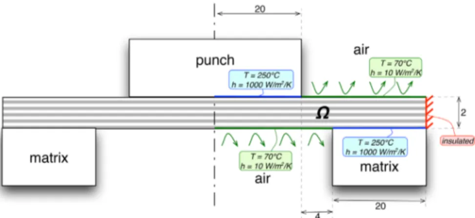
3.3. Application to Industrial Nonlinear Case

3.3.1. Problem Definition

The proposed ADI resolution method was applied to an industrial case representative of the thermostamping process. A 2 mm thick laminate comprised of 16 anisotropic plies stacked on a 0, 90

s

 

  sequence is considered.

The temperature dependant thermal properties are adapted from carbon fibre reinforced PEEK and are given in Table 4. The initially hot laminate (at 400 C )

comes in contact with a cold matrix and punch set, as illustrated in Figure 10, at time t=0 s.

The 2D heat transfer problem is solved using (i) a full 2D resolution in COMSOL (ii) the presented alternate direction implicit (ADI) method, and (iii) a series of independant one-dimensional through thickness problems. In the ADI method, the Pm problem consists of a 1D homogenized through thickness

problem. Because of the 0, 90

s

 

  stacking sequence, the in-plane thermal

conductivity tensor Ks is isotropic and is an average of the longitudinal and

transsverse properties given in Table 4. Nonlinear resolution is performed in MATLAB over a physical time of 5 s with 150 time steps. In COMSOL, the

exact multiply description is implemented. Using symmetry, only half of the geometry is considered and presented hereunder.

3.3.2. Results and Discussion

Three-dimensional effect. The problem is nonlinear, and, as visible in Figure 11, highly three-dimensional at the vicinity of the shear edge (between the

(19)

Figure 9. Maximum error between the temperature fields computed with COMSOL using a 3D model and with the presented approach vs. thickness to radius of curvature ratio h R . The error is computed at final time t=20 s. As h R increases, the metric tensor g becomes not constant through thickness, and the separated form resolution fails at predicting 3D effects.

Figure 10. Industrial test case geometry and boundary conditions. The problem is solved on the multiply laminate domain Ω.

Figure 11. Industrial test case. Close up on temperature fields at time 3 s computed with the full 2D resolution (up) and the ADI method (down). The three-dimensional effect is partly described with the ADI method.

(20)

Table 4. Material properties used in the industrial case, representative of carbon fibre/ PEEK composite.

Transverse thermal conductivity _{W m}_⋅ −1_⋅_K−1 3

0.42 1 10+ × − ×  T_{ }C

Longitudinal thermal conductivity _{W m}_⋅ −1_⋅_K−1 3

4.0+7.5 10× − ×  T_{ }C

Specific heat 1 1

J kg⋅ − ⋅K− 800+2.25 T×  _{ }C

Density 3

kg m⋅ − 1600 0.2 T− ×  _{ }C

punch and the matrix). Still the proposed ADI method is able to partly discribe this tridimensional effect thanks to the Pm problem that considers in plane

diffusion.

Temperature profiles at three different positions at time t=3 s are plotted

in Figure 12.

• Far from the shear edge (cut CC'), the temperature gradient is mostly through thickness and the three approaches prove efficient at describing the through thickness temperature field.

• In the centre of the shear edge zone (cut AA'), the ADI method enables an accurate recovery of the through thickness profile obtained with the full 2D method. On the contrary, at this position AA', the one-dimensional method highly overestimates the temperature since it does not account for the nearby cold moulds.

• Similarly in the intermediate region over the matrix (cut BB’), the one- dimensional approach under predicts the temperature field. On the contrary, the ADI proposed method, enables a partial description of the three-dimensional effects (±5 C ). Nonetheless, the method results in overpredicting temperature

at height y=1 mm. At this worst position, three-dimensional effects are

enhanced, the decomposition methods fails and this artifact (also visible in Figure 11) cannot be overcome.

Nonlinearity. In addition to this three-dimensional effect, the proposed industrial case is nonlinear, since the properties are temperature dependant. In this nonlinear case, the ADI method still proved efficient at predicting the temperature field. The efficiency of the method is explained by the very smooth non-linearities of the thermal properties used in the test case (see Table 4). Given that this is the case for the majority of industrial thermoplastic composite, the decomposition ADI method will likely be efficient for other industrial materials.

Multiply. Finally, the industrial test case was performed with a 16 plies laminates, with a very harsh 0 ,90_  __{anisotropic stacking. The ADI, which} considers an homogenized in-plane conductivity for the in-plane Pm problem,

still proves efficient at predicting the thermal fields. In conclusion, as far as the heat transfer is concerned, a multiply stacking representative of an industrial blank can be considered as homogeneous through thickness.

(21)

Figure 12. Industrial test. Temper 5 C±  _{ature profiles through thickness at three}

different positions. Plots are at time 3 s for the full 2D resolution, the ADI method and the one-dimensional method.

3.4. Proposed Integration in a Global Procedure

Several thermostamping simulation tools exist which handle the mechanics. This is the case, for instance, of Plasfib [30], Aniform [31] or PAMForm [4]. In order to improve the physical description of these tools, accurate prediction of heat transfer is required. Implementation using the presented method, is possible for several reasons:

1) In these tools, the global time integration scheme is incremental and therefore follows the same scheme as the one described in Section 2.2.2. The iterative time integration procedure is thus consistent between the existing mechanical algorithm, and the proposed heat transfer with operator splitting algorithm.

2) The two-dimensional problem Pm is a standard partial differential equa-

tion. The spatial integration can be integrated using standard numerical methods. The FEM tools developed for the other physics (in the above examples, mechanics) can easily be reused for this heat equation.

3) The problems Pz are independent one-dimensional partial differential

equations. Implementation is straightforward using standard numerical methods (finite difference, finite elements).

4) The through thickness average two-dimensional temperature field T z is

readily available as the solution of the Pm problem at each time step. Thus it

can be used as an input for a rough evaluation of a through thickness equivalent mechanical behavior. Furthermore, should one want a finer mechanical description, the full three-dimensional field is also provided at each time step (Equation (25)).

4. Conclusions

(22)

temperature field in thin shells. It is particularly adapted to simulate temperature effects in thermo-stamping processes. The main contributions of this work are the following:

• An in-plane/out-of-plane decomposition strategy was proposed. The initial 3D heat transfer problem can be solved in two successive steps:

-solving of a series of 1D problems (Pz) with a fine time step and a good

accounting of thermal shocks problems. -solving of one 2D problem (Pm).

The strong potential of this numerical strategy for computational costs reduction was clearly highlighted.

• The applicability of this solving strategy was investigated. Two conditions are to be fulfilled for the model to be predictive:

-a small aspect ratio for conduction dimensionless ratio A that includes both geometrical aspect ratio h L and anisotropy of the conductivity tensor.

-a small thickness to radius of curvature ratio h R.

These two conditions are fulfilled in standard thermo-stamping industrial cases.

• The proposed formulation is such that the problems Pm and Pz are

classical and can be solved within a standard incremental time integration scheme and FEM formulations. Thus, the ADI decomposition can readily be implemented in existing industrial simulation softwares.

Acknowledgements

This study is part of the COMMANDO-STAMP project managed by IRT Jules Verne (French Institute in Research and Technology in Advanced Manufactur- ing Technologies for Composite, Metallic and Hybrid Structures). The authors wish to associate the industrial and academic partners of this project; Respec- tively SAFRAN, Peugeot Citroën Automotive, SOLVAY, CEMCAT, LTN, GeM, LAMCOS and 3SR. Also, fruitful discussions with Philippe Boisse and Nahiene Hamila about the integration in a global procedure are to be acknowledged.

References

[1] Hou, M. (1997) Stamp Forming of Continuous Glass Fibre Reinforced Polypropy-lene. Composites Part A: Applied Science and Manufacturing, 28, 695-702. https://doi.org/10.1016/S1359-835X(97)00013-4

[2] Lessard, H. (2014) Évaluation expérimentale du procédé de thermoformage- estampage d’un composite peek/carbone constitué de plis unidirectionnels. Ph.D. Thesis, Université du Québec à Trois-Rivières, Trois-Rivières.

[3] Karbasian, H. and Tekkaya, A.E. (2010) A Review on Hot Stamping. Journal of Ma-terials Processing Technology, 210, 2103-2118.

https://doi.org/10.1016/j.jmatprotec.2010.07.019

[4] De Luca, P., Lefebure, P. and Pickett, A.K. (1998) Numerical and Experimental In-vestigation of Some Press Forming Parameters of Two Fibre Reinforced Thermop-lastics: APC2-AS4 and PEI-CETEX. Composites Part A: Applied Science and Man-ufacturing, 29, 101-110. https://doi.org/10.1016/S1359-835X(97)00060-2

(23)

[5] Cao, J., Xue, P., Peng, X. and Krishnan, N. (2003) An Approach in Modeling the Temperature Effect in Thermo-Stamping of Woven Composites. Composite Struc-tures, 61, 413-420. https://doi.org/10.1016/S0263-8223(03)00052-7

[6] Pickett, A.K., Quickborner, T., de Luca, P. and Haug, E. (1994) Industrial Press Forming of continuous Fibre Reinforced Thermoplastic Sheets and the Develop-ment of Numerical Simulation Tools. International Conference on Flow Processes in Composites Materials, Galway, 7-9 July 1994, 356-368.

[7] Thomann, U.I., Sauter, M. and Ermanni, P. (2004) A Combined Impregnation and Heat Transfer Model for Stamp Forming of Unconsolidated Commingled Yarn Preforms. Composites Science and Technology, 64, 1637-1651.

https://doi.org/10.1016/j.compscitech.2003.12.002

[8] Hamila, N., Boisse, P. and Chatel, S. (2009) Semi-Discrete Shell Finite Elements for Textile Composite Forming Simulation. International Journal of Material Forming, 2, 169-172. https://doi.org/10.1007/s12289-009-0518-5

[9] Ten Thije, R.H.W., Akkerman, R. and Huétink, J. (2007) Large Deformation Simu-lation of Anisotropic Material Using an Updated Lagrangian Finite Element Me-thod. Computer Methods in Applied Mechanics and Engineering, 196, 3141-3150. https://doi.org/10.1016/j.cma.2007.02.010

[10] Saetta, E. and Rega, G. (2014) Unified 2D Continuous and Reduced Order Model-ing of Thermomechanically Coupled Laminated Plate for Nonlinear Vibrations.

Meccanica, 49, 1723-1749. https://doi.org/10.1007/s11012-014-9929-6

[11] Bergman, G. and Oldenburg, M. (2004) A Finite Element Model for Thermome-chanical Analysis of Sheet Metal Forming. International Journal for Numerical Me-thods in Engineering, 59, 1167-1186. https://doi.org/10.1002/nme.911

[12] Surana, K.S. and Phillips, R.K. (1987) Three Dimensional Curved Shellnite Ele-ments for Heat Conduction. Computers & Structures, 25, 775-785.

https://doi.org/10.1016/0045-7949(87)90169-6

[13] Surana, K.S. and Abusaleh, G. (1990) Curved Shell Elements for Heat Conduction with p-Approximation in the Shell Thickness Direction. Computers & Structures, 34, 861-880. https://doi.org/10.1016/0045-7949(90)90357-8

[14] Rolfes, R. and Teßmer, J. (2001) 2D Finite Element Formulation for 3D Tempera-ture Analysis of Layered Hybrid StrucTempera-tures. NAFEMS Seminar: Numerical Simula-tion of Heat Transfer, Wiesbaden, 9-10 May 2001, 1-5.

[15] Do Carmo, D.A. and De Faria, A.R. (2015) A 2D Finite Element with through the Thickness Parabolic Temperature Distribution for Heat Transfer Simulations In-cluding Welding. Finite Elements in Analysis and Design, 93, 85-95.

https://doi.org/10.1016/j.finel.2014.09.005

[16] Bognet, B., Bordeu, F., Chinesta, F., Leygue, A. and Poitou, A. (2012) Advanced Si-mulation of Models Defined in Plate Geometries: 3D Solutions with 2D Computa-tional Complexity. Computer Methods in Applied Mechanics and Engineering, 201-204, 1-12. https://doi.org/10.1016/j.cma.2011.08.025

[17] Chinesta, F., Leygue, A., Beringhier, M., Nguyen, L.T., Grandidier, J.-C., Schreer, B. and Pesavento, F. (2013) Towards a Framework for Non-Linear Thermal Models in Shell Domains. International Journal of Numerical Methods for Heat & Fluid Flow, 23, 55-73. https://doi.org/10.1108/09615531311289105

[18] Douglas, J. (1955) On the Numerical Integration of by 22 22

u u u x y t

∂ ∂ ∂

+ =

∂ ∂ ∂ Implicit Methods. Journal of the Society for Industrial and Applied Mathematics, 3, 42-65. [19] Douglas, J. and Rachford, H.H. (1956) On the Numerical Solution of Heat

(24)

Conduc-tion Problems in Two and Three Space Variables. Transactions of the American Mathematical Society, 82, 421-439.

https://doi.org/10.1090/S0002-9947-1956-0084194-4

[20] LeVeque, R.J. (2005) Finite Difference Methods for Differential Equations. Univer-sity of Washington, Seattle.

[21] Peaceman, D.W. and Rachford, H.H. (1955) The Numerical Solution of Parabolic and Elliptic Differential Equations. Journal of the Society for Industrial & Applied Mathematics, 3, 28-41. https://doi.org/10.1137/0103003

[22] Strang, G. (1968) On the Construction and Comparison of Difference Schemes.

SIAM Journal on Numerical Analysis, 5, 506-517. https://doi.org/10.1137/0705041 [23] Lions, P.L. and Mercier, B. (1979) Splitting Algorithms for the Sum of Two

Nonli-near Operators. SIAM Journal on Numerical Analysis, 16, 964-979. https://doi.org/10.1137/0716071

[24] Godunov, S.K. and Ryabenkii, V.S. (1987) Difference Schemes: An Introduction to the Underlying Theory. Elsevier Science, Amsterdam.

[25] Thomas, M., Boyard, N., Lefèvre, N., Jarny, Y. and Delaunay, D. (2010) An Experi-mental Device for the Simultaneous Estimation of the Thermal Conductivity 3-D Tensor and the Specific Heat of Orthotropic Composite Materials. International Journal of Heat and Mass Transfer, 53, 5487-5498.

https://doi.org/10.1016/j.ijheatmasstransfer.2010.07.008

[26] Douglas, J. and Seongjai, K. (2001) Improved Accuracy for Locally One-Dimen- sional Methods for Parabolic Equations. Mathematical Models and Methods in Ap-plied Sciences, 11, 1563-1579. https://doi.org/10.1142/S0218202501001471

[27] Faraj, J., Pignon, B., Bailleul, J.L., Boyard, N., Delaunay, D. and Orange, G. (2015) Heat Transfer and Crystallization Modeling during Compression Molding of Thermoplastic Composite Parts. Key Engineering Materials, 651-653, 1507-1512. https://doi.org/10.4028/www.scientific.net/KEM.651-653.1507

[28] Carslaw, H.S. and Jaeger, J.C. (1959) Conduction of Heat in Solids. Clarendon Press, Oxford.

[29] Fachinotti, V.D. and Bellet, M. (2006) Linear Tetrahedral Finite Elements for Thermal Shock Problems. International Journal of Numerical Methods for Heat & Fluid Flow, 16, 590-601. https://doi.org/10.1108/09615530610669120

[30] Guzman-Maldonado, E., Hamila, N., Boisse, P. and Bikard, J. (2015) Thermome-chanical Analysis, Modelling and Simulation of the Forming of Pre-Impregnated Thermoplastics Composites. Composites Part A: Applied Science and Manufactur-ing, 78, 211-222. https://doi.org/10.1016/j.compositesa.2015.08.017

[31] Haanappel, S.P., Thije, R.H.W., Sachs, U., Rietman, B. and Akkerman, R. (2014) Composites: Part A Formability Analyses of Unidirectional and Textile Reinforced Thermoplastics. Composites Part A, 56, 80-92.

https://doi.org/10.1016/j.compositesa.2013.09.009

[32] Benveniste, Y. (2006) A General Interface Model for a Three-Dimensional Curved Thin Anisotropic Interphase between Two Anisotropic Media. Journal of the Me-chanics and Physics of Solids, 54, 708-734.

https://doi.org/10.1016/j.jmps.2005.10.009

[33] Bognet, B., Leygue, A. and Chinesta, F. (2014) Separated Representations of 3D Elastic Solutions in Shell Geometries. Advanced Modeling and Simulation in Engi-neering Sciences, 1, 4. https://doi.org/10.1186/2213-7467-1-4

[34] Hladik, J. and Hladik, P.-E. (1999) Le calcul tensoriel en physique. 3rd Edition, Dunod, Paris.

(25)

Appendix. Arbitrary Curvilinear Shell Description

In this Appendix, the surface operator ∇s is defined in the arbitrary curved

shell domain illustrated in Figure 1. This definition follows the framework adopted by Benveniste [32] in the case of a thin interphase. A similar approach is fully detailed in three dimensions by Bognet et al. [33] in their appendix.

A.1. Mid-Surface Description

Mapping. The reference global cartesian system is denoted as

(

X Y Z, ,

)

with

its origin O. First, the mid-surface Γ of the shell like domain is considered. A position G=

(

X Y Z, ,

)

on this surface Γ is parametrized in a reference

dimensionless coordinate system

(

p q,

)

using the mapping function

[ ]

(

)

(

)

2 3 0,1 : , , , p q G X Y Z  _→ _{Γ ⊂}   → =   φ (27)

This mapping

φ

is such that p and q are dimensionless.

Basis. The natural basis at point G consists of the two tangent vectors

0 , p p p ∂ = = ∂ φ e φ and 0 , q q q ∂ = = ∂ φ e φ

where the standard comma notation denotes derivation.

Metric tensor. The first fundamental metric tensor of this 2D surface writes, in the local basis,

(

0 0

)

0 0 0 0 0 0 0 0 0 , . p q p p p q p q q q  ⋅ ⋅  =  _⋅ _⋅     e e e e e e g e e e e

The unit normal to the tangent surface at point G is also defined as

0 0 0 0 . p q p q ∧ = ∧ e e n e e (28) The second order tensor b, representing the second fundamental form,

which components are defined as bij =ei j, ⋅n, ∀ ∈i

{ }

p q, ,∀ ∈j

{ }

p q, gives the

local mean curvature

( )

1 trace 2

H= b

and Gaussian curvature

( )

det

K= b

of the surface Γ .

A.2. Shell Domain Parametrization

(26)

described in Figure A1. The projection G of M on the mid-surface Γ is first defined. Therefore, OM  =OG+GM . G is parametrized using the mapping (27) and the third dimensionless coordinate

GM r h ⋅ =  n

is defined, where h is the local thin shell thickness. It quantifies the distance between M and the mid-surface Γ . Thus the coordinate r∈ −

[

1 2 ,1 2

]

is

also dimensionless. In summary, the shell domain mapping writes

[ ]

(

)

(

)

2 1 1 ₃ 0,1 , 2 2 : , , , p q r M p q rh  _{× −} _{→ Ω ⊂}  _ _   _→ ₌ ₊   ψ φ n

Because r is the distance to the mid-surface, the

(

p q r, ,

)

coordinate sys-

tem is parallel curvilinear as defined by Benveniste [32].

Basis. At point M , the natural basis associated to this curvilinear coordinate system consists of the three vectors

Figure A1. Illustration of the mapping used to parametrize the shell domain Ω_{. The} position M =

(

X Y Z, ,

)

in the physical Euclidean space is obtained from the dimensionless coordinates

(

p q r, ,

)

using: (i) the mid-surface Γ mapping (the function

(

)

: p q, G

(27)

26

( )

0 , , , , 0 , , , , , . p p p p p r p q q q q q r q r r r h r r h r h = = + = + = = + = + = = e ψ φ n e e e ψ φ n e e e ψ n (29) Metric tensor. The symmetric fundamental metric tensor g is described in

terms of its coordinates gij where i∈

{

p q r, ,

}

and j∈

{

p q r, ,

}

. By defini-

tion

.

ij i j

g = ⋅e e

Because the system is parallel curvilinear, g_pr =g_qr =0. Moreover, Equation (29) gives

2 2

rr

g =hn n⋅ =h because n is a unit vector.

Following Equation (64) in [33], the component gpp, gpq and gqq write

1

{ }

0 2 2 2 , , 2 , , , , ij ij ij ij i j g =g − rhb +r h c +r h h ∀ ∈i p q ∀ ∈j p q (30)

where the second order tensor c represents the extrinsic third fundamental form. This equation shows that the local metric tensor g is obtained as a

correction of the metric tensor 0

g at the mid surface Γ . This correction

depends on the distance rh from Γ and gets larger as the curvature b

increases. But it also depends on the shell thickness variation

( )

2 ,ij

h that may

occur in the case of blanks with ply drops.

In the case where the radii of curvature of the surface Γ are large compared to the shell thickness h, the second term is negligible compared to the first one. Because cij is a product including the curvature bij (see for instance Equation

(59) by Bognet et al. [33]), the third term also vanishes besides 0

ij

g when the

curvature of Γ tends to 0. If, in addition, the shell thickness variations h,i are

small, the last term can also be neglected. Then, the fundamental metric tensor in the shell reduces to

[ ]

0 0 0 0 0 2 2 0 0 0 0 0 0 pp pq qp qq g g g g h h   _ _     _{ } =_ _=           g g (31)

and is thus independent of the through thickness position r in the shell. Furthermore, the inverse of this metric tensor is also block-diagonal and writes

( )

[ ]

1 0 1 2 0 . 1 0 h − − _ _      =       g g (32)

A.3. Surface Differential Operators

Gradient. Following [34], the gradient of a scalar β_{is a first order tensor.}

1_{The expression (30) for}

ij

g differs from that of [33] because, in our case, er=hn, where h

(28)

In the contravariant basis

(

e e ep, q, r

)

, it writes , 1 , , p q r β β β β −     ∇ = _ _     g

which can be decomposed, using Equation (32) into an in-plane and an out-of- plane term: , 2 1 s r r h β β β ∇ = ∇ + e

where the surface gradient ∇sβ writes, in the basis (ep, eq):

( )

₀ 1 _, , . p s q β β  − _β  ∇ =__ _     g (33) In the case where the out-of plane coordinate r is redimensionalized, as z=hr, the normal vector ez =her =n, and

, .

s z z

β β β

∇ = ∇ + e

As described in section 2.1.2, for a conductivity tensor which has a principal direction in the out of plane direction (Equation (3)), the flux in-plane/out-of- plane decomposition (4) is recovered.

Divergence. First, the following scalar magnitude is defined: