HAL Id: hal-00878543
https://hal.archives-ouvertes.fr/hal-00878543
Submitted on 30 Oct 2013
HAL is a multi-disciplinary open access
archive for the deposit and dissemination of
sci-entific research documents, whether they are
pub-lished or not. The documents may come from
L’archive ouverte pluridisciplinaire HAL, est
destinée au dépôt et à la diffusion de documents
scientifiques de niveau recherche, publiés ou non,
émanant des établissements d’enseignement et de
A multi-resolution image reconstruction method in
X-ray computed tomography
Marius Costin, Delphine Lazaro-Ponthus, Samuel Legoupil, Philippe
Duvauchelle, Valerie Kaftandjian
To cite this version:
Marius Costin, Delphine Lazaro-Ponthus, Samuel Legoupil, Philippe Duvauchelle, Valerie Kaftandjian.
A multi-resolution image reconstruction method in X-ray computed tomography. Journal of X-Ray
Science and Technology, IOS Press, 2011, 19 (2), pp.229-247. �hal-00878543�
A 2D Multiresolution Image Reconstruction Method in X-ray
Computed Tomography
Marius Costin
a,b,∗, Delphine Lazaro-Ponthus
a, Samuel Legoupil
a,
Philippe Duvauchelle
band Val´
erie Kaftandjian
b aCEA, LIST, F-91191 Gif-sur-Yvette, France
bINSA Lyon, CNDRI, F-69621 Villeurbanne, France
Abstract
We propose a multiresolution X-ray imaging method designed for non-destructive test-ing/evaluation (NDT/NDE) applications which can also be used for small animal imaging studies. Two sets of projections taken at different magnifications are combined and a mul-tiresolution image is reconstructed. A geometrical relation is introduced in order to combine properly the two sets of data and the processing using wavelet transforms is described. The ac-curacy of the reconstruction procedure is verified through a comparison to the standard filtered backprojection (FBP) algorithm on simulated data.
Keywords: X-ray CT, image reconstruction, multiresolution.
1
Introduction
In micro and nano computed tomography (CT) studies, the need for higher resolution images is constantly increasing. State-of-the-art X-ray nanoCT systems are capable of providing images with nominal pixel sizes of hundreds of nanometers. At this scale, for the most applications transversal truncation is inherent due to the size of the sample which is larger than the field of view (FOV). Therefore, a direct usage of the classical FDK (Feldkamp Davis Kress) [19] algorithm is not adequate because it requires non-truncated projections.
Several methods were proposed to solve this problem by reconstructing only a region of interest (ROI) inside an object. In the inverse problems theory this is known as the interior problem. In two dimensions (2D), the direct application of the filtered backprojection (FBP) formula leads to an inexact solution, because of the non-locality of the ramp filter. Accurate reconstruction methods based on the backprojection of the first derivative are presented in several recent papers [14, 30, 43, 44, 49]. Their main advantages are the true locality and the ability to reconstruct accurately ROIs from truncated or contaminated data sets, but the inversion of the resulting Hilbert transformed image is costly in terms of computation time. In configurations where the ROI is fully inside the object the solution is not unique, hence this method does not provide an answer to all the possible truncations. The inversion using the backprojection of the second derivative of the projections, called λ-tomography [17, 18, 45, 46], produces only approximative images with amplified edges that is unsuitable for most applications.
Apart from the purely mathematical research in the inversion problem, approximative methods were developed in order to overcome the transversal truncation. Lewitt [27] proposed several pro-jection extension schemes and his implementation of a simple completion method gives good results with reasonable computational efforts. The analysis in [41] suggests that his method outperforms elliptical or cosine extrapolations, but introduces an asymmetric distortion and is more computa-tionally intensive. Because the projections are not independent, some consistency conditions can be imposed in the process of extrapolation. Most implementations use the Helgason-Ludwig con-ditions and in literature several improvements are presented [20, 26, 27], but all of them are less accurate than the two step Hilbert transform method [14, 30, 49]. However, in cases of purely inte-rior truncation, the completion methods do provide better results since the solutions obtained with the Hilbert method are not stable.
Another way to overcome the transversal truncation problem is the so-called ”zoom-in CT”. It consists of a combination of two sets of projections, one in a position where the object is fully inside the FOV and the second one focused on the ROI. Nalcioglu [29] developed a method for the parallel beam case where only the ROI data is back-projected. In a pre-processing step, the projection data is corrected in order to reduce the artifact due to truncation by using a coarser image which completely covers the object. For the fan-beam and cone-beam cases, a method called reconstruction/reprojection was developed [41]. In a first step, a small set of projections are collected and reconstructed so that the object is globally known. The second step consists of an acquisition at a higher resolution at a position where the projections are transversally truncated. These are then extended with a forward projection procedure through the previously reconstructed object. Ramp filtering is applied on the global sinogram, prior to the reconstruction of a desired ROI. Several other papers [8, 11, 12, 42] describe reconstruction methods very similar to the one described in [41]. For the small animal imaging applications, Cho et al. [9] implemented a PI-line-based back-projection filtration algorithm (BPF), which uses only local data and provides images of a quality comparable to full data reconstructions. A variation of the reconstruction/reprojection idea was proposed by Azevedo in [2]. The low resolution data is combined with the high resolution data in the Radon space and the claim is that faster and more accurate reconstructions can be achieved. Recently, Knaup et al. [25] proposed efficient methods for ROI imaging with and without backprojecting the low resolution data.
Unlike all the previously mentioned algorithms, our method aims at reconstructing the entire object, not only the ROI. This is because the targeted objects for our studies can have multiple levels of details. For a lot of applications it is necessary to study the coarse features of a large object and to focus on a certain ROI.
We propose a method which associates a zoom-in acquisition with a multiresolution reconstruc-tion. A proper rearrangement of the ray integrals at the coarse resolution allows to create a global sinogram used as input in our algorithm. Since the resulting sinograms are very large, we need a fast reconstruction. For projections in the order of several thousands of pixels, the standard recon-struction by FBP is time consuming and algebraic methods are hardly feasible. In order to handle the timing constraints we accelerated the reconstruction process by using a wavelet decomposition approach.
The remainder of this article is organized as follows. Next section presents our reconstruction algorithm and section 3 describes the materials and methods used. The results are presented and discussed in section 4, before concluding in Section 5.
2
Proposed Algorithm for Multiresolution Image
Reconstruc-tion
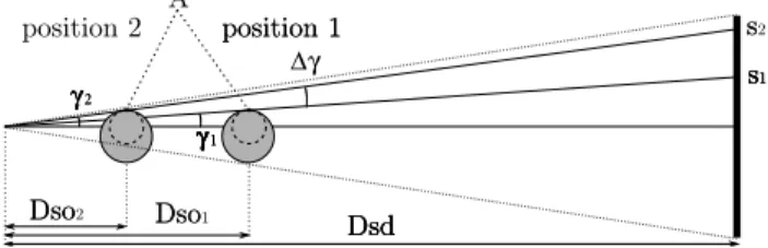
We propose a method in which we combine a zoom-in CT acquisition with multiresolution pro-cessing, using the wavelet theory. Originally applied for denoising and compression purposes [1], the use of wavelet theory in the tomographic inversion started to be investigated in [21, 23, 35–38]. We distinguish two main approaches in the use of the multiresolution concept, depending on its place along the inversion process. First, it can be used in the projection space, as in [22, 32, 33] in order to optimize the projection sampling for local tomography. A similar method is to replace only the ramp filtering step of the FBP algorithm with a wavelet ramp filtering as in [47, 48]. The second approach is to adapt the filtering and the backprojection steps in order to recover directly from the sinograms the set of 2D wavelet coefficients corresponding to the imaged object. A 2D inverse wavelet transform is applied on the resulting data in order to recover the tomographic image [3–6,15,31,39]. For more details on the mathematical basis the reader should refer to [13,28]. In our method we use multiresolution processing on both the projection and the reconstructed images. In a zoom-in CT setup as depicted in figure 1, two sets of projections are acquired at position 1 and position 2, respectively. For both positions, the acquisition is performed equiangularly over a circular trajectory.
Fig. 1: Top view of the zoom-in CT setup. The dashed circle represents the ROI, s1and s2indicate
two rays passing through the same point A in the two scanning positions.
The magnification factors at positions 1 and 2 are defined by mf1 = DsoDsd1 and mf2 = DsoDsd2
respectively, where Dsd is the source-to-detector distance and Dso is the source-to-object distance. The two positions are related by a zoom ratio of zr =mf2
mf1.
We consider a ROI either inside or crossing the boundary of the imaged object, but its center must correspond to the rotation axis. Position 1 is chosen in such a way that the object is fully inside the FOV at any projection angle. For the second acquisition, the object is moved towards the X-ray source along the beam axis. The spatial resolution inside the ROI is fixed by the zoom ratio, and the maximum ROI size is limited by the FOV at the second position.
The notations and conventions regarding the CT setup are similar to the ones used by Kak and Slaney in [24]. We consider the object fixed and the fan beam rotating counterclockwise at an angle
β measured from the initial point. A ray is identified by this angle β and a pixel sk = nkα which
defines the distance to the beam axis. The set of projections (i.e. the sinogram) is denoted p and a ray in this set is denoted p(β, s). The detector pixels range between −na and na, with a = 0
identifying the beam axis, and α represents the pixel size of the detector. The angle of the ray with respect to the beam axis is computed as γ = arctan( s
Dsd). Its values are in the interval [−γa, γa]
We reconstruct a pseudo-3D volume by combining a stack of 2D slices. In the following we present the algorithm and the results for one horizontal slice, hence the 2D case. The procedure is applied similarly for all the horizontal planes.
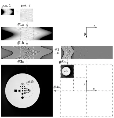
Our method is based on the classical fan beam FBP algorithm in combination with a multires-olution processing and we denoted it ASDIR (Approximate Single Detail Image Reconstruction). It consists of four consecutive steps enumerated below and illustrated in figure 2:
#1 Sinogram creation
#2 Wavelet transform of the sinogram #3 Multiscale backprojections
#4 Image recovery
Fig. 2: Synthesis sketch of the proposed method. The ROI is indicated by the dashed rectangle in the sinogram and by the dashed circle in the reconstructed image.
2.1
Sinogram Creation
In the first step we combine the two sinograms p1 and p2into a single larger one, denoted p. This
process can be considered as an extension of the truncated projections acquired at the zoomed position. Assuming a detector of N1 pixels, we create a virtual detector of N2 pixels, with N2 =
zr· N1. The central part of the extended sinogram p is a point by point copy of the sinogram p2,
and the exterior points are computed from p1.
In order to reduce the acquisition time and the exposure, we chose to measure zr times less angular projections for the low resolution sinogram p1. This reduction is of the same order as the
scaling in the transversal direction and depending on the required precision outside the ROI, it could be furthermore increased. The sampling pattern is therefore nonuniform on both the transversal and the angular directions.
Considering this type of acquisition configuration, the simplest extension is to scale the sinogram
p1 and to interpolate the missing points, independently for each β. But for a divergent beam as in
our case, this approach is not correct because the ray integrals p2(βk, sj)|sj=zr·si and p1(βk, si) are
measured over different paths, hence they have different values. This fact is illustrated in figure 1, where the point A is crossed by different rays at the two positions. However, for the circular scanning trajectory it is possible to identify the corresponding ray which passes at the same incidence angle through the point A in a different projection taken at a neighboring β. For this purpose, we derived two formulas to compute the correct position of the corresponding ray integral in the sinogram. More precisely we want to find the functions g1 and g2which describe the correspondence between
the rays at position 1 and position 2 respectively {
β1= g1(β2, s2) s1= g2(β2, s2)
. (1)
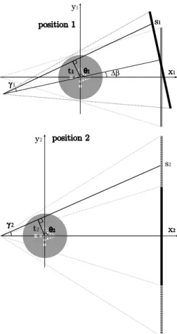
Consider two coordinate systems with the origin on the rotation axis at the two positions, as in figure 3. A ray is described by a line equation of the form
t = x cos θ + y sin θ (2)
where t is the distance from the origin to the line and θ is the angle measured from the x axis to the perpendicular on the line.
In order to identify the same ray in the two systems it is sufficient to impose the following
conditions {
t1= t2 θ1= θ2
. (3)
Based on these relations and using geometrical arguments we compute β1= β2+ arctan ( s2 Dsd ) − arcsin(Dso2 Dso1sin(arctan( s2 Dsd)) ) s1= Dsd tan [ arcsin ( Dso2 Dso1sin(arctan( s2 Dsd)) )] . (4)
With the two relations in (4), we synthesize the first step of our method as
p(β, s)|β=β2,s=s2 =
{
p2(β2, s2), |s| ≤ N21α p1(β1, s1), N21α <|s| ≤ N22α
. (5)
The values computed with the relations in (4) may not be integer to match the exact position of a measured ray in p1(β1, s1). Because a rounding of these values could introduce small discontinuities
in the extended sinogram, we apply a bilinear interpolation between four neighboring points. A small offset in the gray values can still be present after the interpolation which we correct with a simple registration procedure. In order to ensure a smooth transition between the ROI and
Fig. 3: Sketch of the same ray in the two coordinate systems.
the exterior part, we add an offset to the pixels outside the ROI such that the derivative of the projection is continuous. The offset is added only to several neighboring pixels and its value decreases exponentially to zero towards the exterior. The errors which can be introduced by the interpolation are small and the image is affected mainly outside the ROI. Inside the ROI the image is only indirectly affected by the ramp filtering and to a very small extent. This procedure also reduces the effect of discontinuities produced by a geometrical misalignment between the two scan positions.
After the enlarged sinogram is created, the FBP convolution (at the high resolution) is applied to the extended sinogram. With our notations we write this step as
pwf(β, s) = [ Dso2 √ Dso2 2+ s2 p(β, s) ] ∗ h(s) (6)
where H(ω) is the Fourier transform of h(s) and H(ω) = {
|ω|, |ω| ≤ 0.5
0, |ω| > 0.5 . In the case of objects containing sharp transitions a smoothing may be necessary and this is implemented by a
supple-mentary convolution with a window function. A list of such functions and their effect is presented and discussed in [7].
The region corresponding to the ROI is saved as a separate array denoted by pwf ROI and it
serves for the reconstruction of the high resolution part.
2.2
Wavelet Transform of the Sinogram
Each angular projection of the enlarged sinogram is decomposed into approximation and wavelet coefficients following the concept of MRA, as described by Mallat [28]. For a decomposition at the resolution 2j (j∈ {1, ..., J}) the approximation coefficients are obtained with
A2jpβ = (⟨ pwf(β, s), ϕ 2j(s− 2jn) ⟩) n∈Z∗ = ((pwf(β, s)∗ ϕ2j(−s) ) (2jn))n∈Z∗ (7)
where the scaling function ϕ acts as a low-pass filter, which is followed by a sampling at the rate 2j. The detail coefficients are obtained by computing
D2jpβ = (⟨ pwf(β, s), Ψ 2j(s− 2jn) ⟩) n∈Z∗ = ((pwf(β, s)∗ Ψ2j(−s) ) (2jn))n∈Z∗ (8)
where the wavelet Ψ acts as a bandpass filter and it is followed by a sampling at a rate of 2j.
We chose the biorthogonal 4.4 wavelet (or Cohen-Daubechies-Feauveau 9/7) [13] for its good approximation of images with a low number of coefficients [10]. Depending on the image size and the final image quality, different levels of decomposition can be applied, a good compromise being
zr− 1. Each level of DWT consists of an in-place transform, the approximation coefficients are
stored to the left and the details to the right, as illustrated in the middle row of figure 2.
2.3
Multiscale Backprojections
The third step of our method consists of two backprojections which will combine in the final image recovery. For the coarse resolution, we backproject the approximation coefficients from the previous step by using AJf (x, y) = ∫ 2π 0 ( 1 UAJ(x, y, β) )2 AJpβ(sJ) dβ (9)
where f is the function to be reconstructed, UAJ(x, y, β) =
Dso/J +x sin β−y cos β Dso/J , sJ=
1
UAJ(x,y,β)(x cos β+ y sin β) and J is the number of decomposition levels of the DWT.
For the ROI which contains the high resolution part, we backproject the array pwf ROI, saved in the first step fROI(x, y) = ∫ 2π 0 ( 1 UD(x, y, β) )2 pwf ROIβ (sxy) dβ (10)
2.4
Image Recovery
A CT image of N2×N2pixels is recovered by combining the two subimages obtained in the previous
step and we can divide this procedure in three parts. First, the AJ sub-image is used as the set
of approximation coefficients for a 2D separable wavelet decomposition for which we consider all the detail coefficients being zero. Second, this resulting image is inverted by using the 2D inverse DWT created with the same mother wavelet as for the decomposition of the sinogram. Third, the high resolution sub-image fROI is superposed onto its corresponding place in the final image f
0.
We replace pixel by pixel the values corresponding to the ROI and because they have the same origin, i.e. the enlarged sinogram, the gray values are similar and therefore the transition at the ROI border is smooth. For this reason, no registration procedure is needed and the recovered image has correct gray values inside and outside the ROI.
3
Materials and Methods
3.1
Simulated Configuration
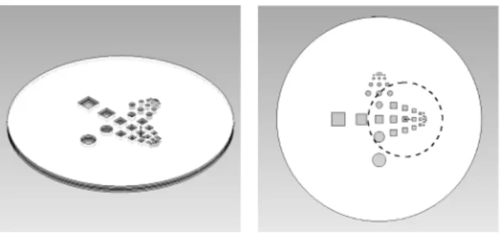
Because our application targets NDT applications, we created a special numerical disk phantom containing holes with decreasing sizes. The Shepp-Logan phantom [40] which is traditionally used for the CT assessment is not well suited for our case because it does not contain similar features to compare the results for the ROI with the exterior. For this purpose we created two patterns of holes with similar sizes, one inside the ROI and the second outside it. In order to evaluate different types of artifacts, one was modeled with rectangular holes and the second with circular holes.
The exterior diameter of the disc measures 15.00 mm and the diameters of the circular holes have the following values: 1.00 mm, 0.80 mm, 0.60 mm, 0.50 mm, 0.40 mm, 0.30 mm, 0.20 mm, 0.10 mm, 0.05 mm, 0.025 mm. The squared holes have exactly the same values for edges and the distances between holes are similar, ranging from 0.80 mm to 0.025 mm. For the holes smaller than 0.60 mm we added transversally pairs of identical holes, as depicted in figure 4.
Fig. 4: Disc phantom with the ROI indicated by the dashed circle (in the top-view drawing). We considered an off-centered ROI having a diameter of 5.55 mm and the origin at the center of the 0.40 mm square hole, as indicated in figure 4. The phantom was modelled as a CAD (computer-aided design) object and a triangularized version saved as a stl file was used as input to the simulation software VXI [16]. Two full scans were simulated with a set of 300 projections for the first position and respectively a set of 1200 projections for the second one. The computations were
performed without including the scattering effect, with a monochromatic source of 70 keV photons, for a disc made of aluminum. The detector contains 1120 pixels with a pixel size of 100µm. The two scanning positions are at Dso1= 72 mm and Dso2= 18 mm for a distance source to detector
of Dsd = 360 mm, hence the magnification factors are 5 and 20. With this choice of parameters, the zoom ratio amounts to 4. We reconstruct images of 4480×4480 pixels with a nominal pixel size of 5µm. With this configuration the sampling is four times higher than it would be possible at position 1, i.e. reconstructed images of 1120×1120 pixels with a nominal pixel size of 20 µm.
3.2
Comparison with alternative reconstruction methods
In order to assess the reconstructions performed with the proposed algorithm, a reference image was created to serve for comparisons. A full scan was simulated at position 2 with a detector of 4480 pixels. The resulting sinogram has exactly the same dimensions as our enlarged one, but the forward projection is performed for all the pixels, providing a high resolution for the whole image, not only for the ROI as in our case. The image is reconstructed with the standard FBP algorithm and is denoted in the following ”reference FBP”.
We distinguish two features in our algorithm which we want to evaluate. First, the extension of the projections with the proposed relation, which is best evaluated by reconstructing the enlarged sinogram with the FBP algorithm. The resulting image is denoted ”extended FBP”. The second is the multiresolution processing which produces an approximation image outside the ROI, but several times faster than the FBP algorithm. This image is denoted in the following ”ASDIR”.
An alternative reconstruction method which does not use the wavelet transform can be synthe-sized in the following steps:
#1 Reconstruct the low resolution data p1
#2 Extend the high resolution data p2 with the low resolution data p1, as described in section 2.1
#3 Reconstruct the ROI from the extrapolated sinogram
#4 Combine the low resolution and ROI reconstructions in the image space The image reconstructed with this algorithm is denoted in the following ”ALT”.
3.3
Spatial Resolution and Noise Considerations
The spatial resolution aspect was addressed by an analysis of the smallest details in the recon-structed images. A rough estimation of the spatial resolution was performed with the help of profile plots through the different series of holes. The accuracy of the reconstructions was assessed quantitatively by computing the mean squared error (MSE) as
M SE = 1 NxNy Nx ∑ y=1 Ny ∑ x=1
[I(x, y)− Iref(x, y)]2 (11)
where Nxand Ny represent the dimensions of the area used for computation and I is the image to
be compared to the reference image Iref. We computed separately the values over homogeneous
The stability of the method with respect to noise was verified by several comparisons to the refer-ence FBP reconstruction. We simulated forward projection data with beams containing 103, 104, 105
and 5× 10⁵ photons per ray. For each case, 25 identical sinograms were generated and a
Poisso-nian noise was added. The MSE was computed independently for each plane, with respect to the noiseless image. The average value of MSE was calculated separately for the whole image and for the ROI respectively. Another parameter, the signal-to-noise ratio (SNR) was calculated indepen-dently for all the pixels as the ratio between the mean value and the standard deviation over the 25 reconstructed images. The final SNR value is the average over all the pixels of the region.
3.4
Timing Considerations
In the FBP algorithm the most time consuming part is the backprojection. Our method improves significantly the reconstruction speed because we backproject only a fraction of the points needed by the classical FBP algorithm. We can estimate this gain in the computation time by an area ratio. We denote with sf the speedup factor, calculated as the ratio between the total number of pixels in the image to the number of backprojected pixels with our method. For a wavelet decomposition on J levels and a zoom factor zr, it can be written as
sf = [ 1 4J + 1 2zr ]−1 . (12)
In the above formula, the terms represent ratios between the number of points which are backpro-jected to the total number of points of the image. The first term corresponds to the backprojection of the global approximation while the second to the backprojection of the ROI. We remark the fact that for reasonable zoom in CT configurations zr and J have small values, not larger than 16. The value computed with the above relation is interpreted as an improvement of sf times in the reconstruction speed as compared to the standard FBP applied for the combined sinogram.
4
Results and discussion
A first remark is that the enlarged sinogram obtained after the first step can be directly inverted with a simple FBP implementation. But this would not be efficient because the images are very large and the region outside the ROI is artificially oversampled. With our algorithm we optimize the reconstruction process by avoiding unnecessary backprojections which are costly in terms of computation time. The wavelet processing brings the advantage of a good approximation for the region outside the ROI.
Because the results for the ROI are the most important, we present first a comparison with images obtained for it. In figure 5 we depict reconstructions of the ROI for three cases: truncated data, before and after replacing the fROI subimage. The first row of figure 5 is only an illustration
of the distortions produced by transversal truncation. In the profile plot along the dashed horizontal line the cupping artifact due to truncation is clearly visible, together with a reduction of the contrast ratio. The second row of figure 5 displays the ROI obtained with the coarse resolution from the backprojection of the approximation coefficients AJf . After the last step of our method consisting
of the replacement of the ROI, the result is more accurate, as depicted in the bottom row of figure 5. With these profile plots we show only partially the differences between the intermediate and the final step. They will be emphasized for the smallest holes in a following paragraph, at the analysis
0 0.5 1 1.5 2 0 555 1110 G r ay V al u e Pixel No. ideal FBP truncated 0 0.2 0.4 0.6 0.8 1 1.2 1.4 0 555 1110 Gray Value Pixel No. ideal intermediate 0 0.2 0.4 0.6 0.8 1 1.2 1.4 0 555 1110 Gray Value Pixel No. ideal ASDIR
Fig. 5: ROI (dashed circle) and profile plots through its center, along the horizontal dotted line. Top row: FBP from truncated projections. Middle row: intermediate image after applying the 2D inverse DWT. Bottom row: ASDIR.
of the spatial resolution. We point out that this comparison is equivalent to the comparison of similar features inside and outside the ROI which will be presented in figure 7.
Reconstructed images with the three methods are displayed in figure 6. In order to verify the continuity at the boundary of the ROI, we plotted a profile through the central vertical line, indicated with the dashed line in the (rotated) magnified view on the upper right corner of the figure. The middle part of this line crosses the ROI, and as expected the transition is smooth for both the extended FBP and the ASDIR images.
Regarding the spatial resolution aspect, we investigated first the monoresolution image (reference FBP) and secondly the multiresolution ones (extended FBP and ASDIR). For a nominal pixel size of 5µm, we expect to clearly identify the 25 µm holes. Moreover, in the reference image we should be able to distinguish the rectangular from the circular shapes. The results shown in the first column
0 0.2 0.4 0.6 0.8 1 0 350 700 1050 1400 Gray Value Pixel No. reference FBP 0 0.2 0.4 0.6 0.8 1 0 350 700 1050 1400 Gray Value Pixel No. extended FBP 0 0.2 0.4 0.6 0.8 1 0 350 700 1050 1400 Gray Value Pixel No. ASDIR
Fig. 6: Reconstructed images of the disc phantom and several profile plots along the central vertical line. The support of the plots is indicated with the dotted line in the magnified view (rotated) on the upper right corner. Top row: reference FBP image. Middle row: extended FBP. Bottom row: ASDIR.
in figure 7 confirm our assumptions with the remark that the circular holes are slightly deformed due to the angular undersampling and the asymmetry of the features of the object. The chosen configuration does not meet the sampling condition [7] of having M ≥ π2N angular projections,
where N represents the number of pixels in the detector. Such a large number of projections is prohibitive in experiments and our aim was to simulate a case close to our experimental set-up. A more detailed study on the angular sampling is an objective of our future work.
In the multiresolution images, we expect a resolution inside the ROI similar to the one of the reference image and at most four times lower outside the ROI, value given by the zr factor. The
0 0.2 0.4 0.6 0.8 1 0 10 20 30 40 50 60 G r ay V al u e Pixel No. reference FBP 0 0.2 0.4 0.6 0.8 1 0 10 20 30 40 50 60 G r ay V al u e Pixel No. extended FBP 0 0.2 0.4 0.6 0.8 1 0 10 20 30 40 50 60 G r ay V al u e Pixel No. ASDIR 0 0.2 0.4 0.6 0.8 1 0 10 20 30 40 50 60 G r ay V al u e Pixel No. reference FBP 0 0.2 0.4 0.6 0.8 1 0 10 20 30 40 50 60 G r ay V al u e Pixel No. extended FBP 0 0.2 0.4 0.6 0.8 1 0 10 20 30 40 50 60 G r ay V al u e Pixel No. ASDIR
Fig. 7: Magnified areas and corresponding profile plots for the smallest details, the 25µm holes, for the three cases: reference FBP, extended FBP and ASDIR. The upper left image indicates the ROI and the position of the magnified areas. The top row contains the circular holes, situated outside the ROI, and the bottom row displays the rectangular holes, situated inside the ROI.
bottom images in the second and third columns of figure 7 prove that inside the ROI we obtain results almost identical to the reference image, hence the resolution is conserved. Outside the ROI, the resolution is degraded, as seen in the upper images, in the second and third columns of figure 7. For a better evaluation, we analyzed the adjacent row of holes which have a diameter of 50 µm. Figure 8 presents magnified views and profile plots along the dashed lines. The features are resolved in both cases and we conclude that the obtained resolution outside the ROI is enough to meet our requirements.
0 0.2 0.4 0.6 0.8 1 0 20 40 60 80 100 120 G r ay V al u e Pixel No. extended FBP 0 0.2 0.4 0.6 0.8 1 0 20 40 60 80 100 120 G r ay V al u e Pixel No. ASDIR
Fig. 8: Extended FBP (left) and ASDIR (right) images: magnified areas outside the ROI containing the 50µm circular holes and the associated profile plots along the dashed line.
An exact computation of the spatial resolution value (SR) in the reconstructed images is beyond the purpose of this paper. Instead, we were able to estimate the bounds of the intervals containing the SR values for the low resolution and for the high resolution regions. As a remark, these values
are highly dependent on the chosen CT geometry and in practice they are degraded by several factors. Taking into account that the 25 µm holes are resolved, we conclude that the resolution inside the ROI is better than 20 line pairs per millimeter (lp/mm) and that it is limited by the pixel size to a value of 100 lp/mm. Outside the ROI, based on the fact that the 50µm holes are resolved and the 25µm ones are not resolved, we compute the limits of the interval to 10 and 20 lp/mm respectively.
Figure 9 displays the reconstruction using the alternative algorithm described in section 3.2. The reconstructed image is highly degraded by streak artefacts and aliasing originating from the
0 0.2 0.4 0.6 0.8 1 0 10 20 30 40 50 60 Gray Value Pixel No. ALT 0 0.2 0.4 0.6 0.8 1 0 20 40 60 80 100 120 Gray Value Pixel No. ALT
Fig. 9: Reconstruction with the alternative algorithm and profile plots through the 25µm and 50 µm holes outside the ROI.
low number of projections used in the first step. We compressed the grayscale in order to emphasize these artefacts and this shows another problem, i.e. a shift of the gray values between the ROI and the rest of the object. In the last step of the algorithm we used a simple registration procedure which shifts the gray values inside the ROI with the difference of the average values computed over homogeneous zones inside and outside the ROI. On the right side of figure 9 the zoomed regions similar to the top row of figure 7 and respectively of figure 8 are displayed with the associated profile plots along the dashed lines. While the smallest holes are completely undistinguishable, the second row is more visible but still worse than ASDIR. The presented image is a reconstruction with a direct implementation of the algorithm described in section 3.2. It would surely give better results with some optimizations and smoothing, but we believe it cannot match the performance of ASDIR. There are three main arguments supporting this statement. First, the number of projections used in the reconstruction is lower for the alternative method compared to ASDIR and therefore the low resolution part of the ASDIR image will contain less artefacts. Second, in the last step of ASDIR, the inverse DWT is applied by considering the detail wavelet coefficients as zero. This has the effect of a low-pass filtering and hence in the case of noisy data the high frequency noise will be reduced. Third, with experimental data the gray values may vary between the acquisitions at the two positions. For best results the alternative algorithm would require an advanced registration procedure in the image space in order to ensure the recovery of the correct values inside and outside the ROI. By contrast, ASDIR needs only a simple and fast registration applied on the sinograms and the final images are correctly recovered without further processing.
The quantitative assessment of the reconstruction quality was performed first on noiseless recon-structions by comparing the ASDIR and ALT images to the reference FBP. For the ASDIR image, in the low resolution region we obtained a MSE of 1.02× 10⁻⁴and for the high resolution region a MSE of 3.8× 10⁻⁷. The error for the ROI amounts to about three times the machine epsilon for the single precision floating point arithmetic. For the ALT image the MSE computed for the low
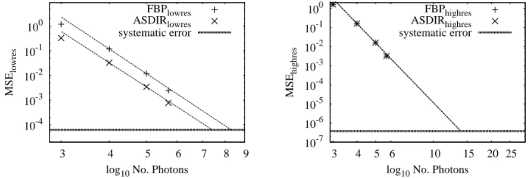
resolution part amounts to 2.12× 10⁻² and for the high resolution part is identical to ASDIR. A second quantitative evaluation was the behavior of the ASDIR algorithm with respect to FBP in the case of noisy data. The average MSE was computed as described in section 3.3 for the noisy reference FBP and noisy ASDIR images with respect to the noiseless reference FBP image. Figure 10 presents on a logarithmic scale the MSE computed for the low resolution part on left and for the high resolution part on right, for the four noise levels (103, 104, 105 and 5× 10⁵ photons). In the first case we remark a lower MSE for our method which is a consequence of the low-pass
10-4 10-3 10-2 10-1 100 3 4 5 6 7 8 9 MSE lowres
log10 No. Photons
FBPlowres ASDIRlowres systematic error 10-7 10-6 10-5 10-4 10-3 10-2 10-1 100 3 4 5 6 10 15 20 25 MSE highres
log10 No. Photons
FBPhighres
ASDIRhighres systematic error
Fig. 10: Average MSE for the low resolution part (outside ROI) and for the high resolution part (inside ROI) in the case of noisy data.
filtering in the last step of the ASDIR algorithm. The four points were fitted in order to show the trend for a larger interval. The plots show also the ”systematic error” which is computed as the MSE for noiseless data. The intersection of the fit with the systematic error marks the point where the Poissonian noise becomes less important than the errors introduced by the ASDIR algorithm. Usually the experimental data is acquired with less than 106 photons per ray and for this reason
we can consider the errors introduced by our method as being negligible. The results for the high resolution part are displayed on the right side of figure 10. As expected, the calculated values of MSE are almost identical for the two images and the trend is showed by a fit. We only remark that in this case the systematic error is much smaller than for the low resolution part.
Another quantitative evaluation was made through the SNR factor. In figure 11 the average values computed for the low resolution region are plotted. The dotted curve represents the theo-retical maximal value of SNR, limit imposed by the Poissonian noise. As in the case of the mean squared error comparison, our method has a better SNR because of the denoising properties of the wavelet transform.
The reconstruction speed was evaluated by taking the fastest time in three runs of the same data set on the same PC, equipped with an AMD Opteron processor running at 2.8 GHz. The best time per horizontal slice amounts to 1848 seconds for the FBP algorithm and 249 seconds for our method. The speedup factor computes therefore to 7.42, close to the expected value of 8 estimated with formula (12). By employing a short scan configuration, the method can be further optimized both in terms of the radiation exposure and of the reconstruction speed, an objective set for our future work. The code used for backprojection was parallelized with OpenMP [34] and showed an almost linear gain with the number of processors used. For a fair comparison, all the results presented in this paper were produced with the non-parallelized version.
1 10 100
3 4 5 6
SNR lowres [dB]
log10 No. Photons FBPlowres ASDIRlowres
Fig. 11: SNR values for the low resolution region.
A major drawback of the presented method is the fact that the extension to the 3D case is impossible for the circular trajectory. On the vertical plane, the projections acquired at the first position are not sufficient for a correct extension. Our idea for ray rearrangement can only be possible for complex source trajectories and is more difficult to implement. However, in the typical experiments with our configuration, the vertical divergence is less than 5 degrees, a value small enough to employ the pseudo-3D reconstruction without introducing important artifacts.
Another disadvantage of our method is the sensitivity to geometric misalignments. The reg-istration procedure employed in the first step reduces this effect but the extent varies with its parameters and more important with the amount of positioning error. As an illustration, in figure 12 we show the ROI and a part of its surrounding area on a image reconstructed from the sinogram
p1including a transversal translation of 12 pixels which represents a spatial misalignment of 60µm.
0.8 0.85 0.9 0.95 1 1.05 1.1 0 50 100 150 200 Gray Value Pixel No. 0.8 0.85 0.9 0.95 1 1.05 1.1 0 50 100 150 200 Gray Value Pixel No.
Fig. 12: Illustration of a geometric misalignment (left) and the effect of the registration procedure (right).
The image on the left shows the reconstruction without the registration procedure and the image on the right shows the reconstruction including the registration. Outside the ROI the image
is distorted in both cases because of the transversal shift. For comparison, the left side image from the bottom row of figure 5 shows the reconstruction from projection data without misalignments. In the case of the uncorrected reconstruction a strong discontinuity is present at the ROI border which is removed by our procedure. This effect is already visible on the CT images but it is proved by the two profile plots along the dotted lines crossing the ROI. The main purpose for using this registration procedure was to ensure a continuous transition at the border of the ROI, especially for experimental data where the gray values may change between the two scans due to intensity variations. For an automated zoom-in acquisition a separate procedure for the correction of geometric misalignments would be required.
5
Conclusions
We presented a multi-resolution tomographic reconstruction method for zoom-in computed tomog-raphy. For a circular scanning trajectory we demonstrated that it is possible to avoid the recon-struction/reprojection approach [41], by a proper extension of the truncated projections with points computed from the measured projections. Our method was validated with simulated data and as proved by the graphs in figure 10, we can conclude that the errors introduced by our algorithm are lower than the Poissonian noise appearing in experimental data. For noisy images our algorithm shows a better behavior than the standard FBP since it reduces the noise in the low resolution region. With a slight loss in spatial resolution outside the ROI, our multi-resolution approach ac-celerates the reconstruction with a significant factor when compared to the FBP reconstruction and the required amount of projection data is reduced.
6
Acknowledgements
We thank the anonymous reviewers for their contribution, in particular for suggesting the compar-ison to the alternative reconstruction described in section 3.2.
References
[1] M. Antonini, M. Barlaud, P. Mathieu and I. Daubechies, Image coding using wavelet transform,
IEEE Trans. on Image Proc. 1 (1992), pp. 205–220.
[2] S. Azevedo, P. Rizo and P. Grangeat, Region-of-interest cone-beam computed tomography, in: International Meeting on Fully Three-Dimensional Image Reconstruction in Radiology &
Nuclear Medicine, 1995.
[3] C. Berenstein and D. Walnut, Wavelets and local tomography, preprint, 1995.
[4] S. Bonnet. Approches Multir´esolution en Reconstruction Tomographique 3D: Application `a l’Angiographie C´er´ebrale, Ph.D. Dissertation, L’Institut National des Sciences Appliqu´ees de Lyon, Images et Systemes, EEA, Lyon, France, 2000.
[5] S. Bonnet, F. Peyrin, F. Turjman and R. Prost, Multiresolution reconstruction in fan-beam tomography, IEEE Trans. Image Proc. 11 (2002), pp. 169–176.
[6] S. Bonnet, F. Peyrin, F. Turjman and R. Prost, Nonseparable wavelet-based cone-beam recon-struction in 3D rotational angiography, IEEE Trans. Med. Imaging 22 (2003), pp. 360–367. [7] T. M. Buzug, Computed Tomography, Springer-Verlag Berlin Heidelberg, 2008.
[8] M. Cho, I. Chun, S. Lee, M. Cho and S. Lee, Trabecular thickness measurement in cancellous bones: postmortem rat studies with the zoom-in micro-tomography technique, Physiol. Meas.
26 (2005), pp. 667–676.
[9] S. Cho, J. Bian, C. Pelizzari, C. Chen, T. He and X. Pan, Region-of-interest image reconstruc-tion in circular cone-beam microCT, Med. Phys. 34 (2007), pp. 4923–4933.
[10] C. Christopoulos, A. Skodras and T. Ebrahimi, The JPEG2000 still image coding system: an overview, IEEE Trans. on Cons. El. 46 (2000), pp. 1103 –1127.
[11] I. Chun, M. Cho, S. Lee, M. Cho and S. Lee, X-ray micro-tomography system for small-animal imaging with zoom-in imaging capability, Phys. Med. Biol 49 (2004), pp. 3889–3902.
[12] I. Chun, S. Lee, M. Cho and M. Cho, Zoom-in micro tomography with the combination of full and limited field-of-view projection data, in: Nuclear Science Symposium Conference Record, 2004, pp. 2962 – 2964.
[13] I. Daubechies, Ten Lectures on Wavelets (C B M S - N S F Regional Conference Series in Applied Mathematics). Soc. Ind. Appl. Math., 1992.
[14] M. Defrise, F. Noo, R. Clackdoyle and H. Kudo, A large class of inversion formulae for the 2D Radon transform of functions of compact support, Inv. Problems 22 (2006), pp. 1037–1053. [15] A. Delaney and Y. Bresler, Multiresolution tomographic reconstruction using wavelets, IEEE
Trans. Image Proc. 4 (1995), pp. 799–813.
[16] P. Duvauchelle, N. Freud, V. Kaftandjian and D. Babot, A computer code to simulate x-ray imaging techniques, Nucl. Instrum. Methods Phys. Res., Sect. B 170 (2000), pp. 245–258. [17] A. Faridani, D. Finch, E. Ritman and K. Smith, Local tomography II, SIAM J. Appl. Math.
57 (1997), pp. 1095–1127.
[18] A. Faridani, E. Ritman and K. Smith, Local tomography, SIAM J. Appl. Math. 52 (1992), pp. 459–484.
[19] L. Feldkamp, I. Davis and J. Kress, Practical cone-beam algorithm, J. Opt. Soc. Am. A 1 (1984), pp. 612–619.
[20] G. V. Gompel, M. Defrise and D. V. Dyck, Elliptical extrapolation of truncated 2D CT projections using Helgason-Ludwig consistency conditions, in: Proceedings of SPIE, 6142 (2006), pp. 1408–1417.
[21] M. Holschneider, Inverse Radon transforms through inverse wavelet transforms. Inv. Problems
7 (1991), pp. 853–861.
[22] T. Hsung and D. Lun, New sampling scheme for region-of-interest tomography, IEEE Trans.
[23] G. Kaiser and R. F. Streater, Windowed Radon transforms, analytic signals and the wave
equation, 1992.
[24] A. Kak and M. Slaney, Principles of Computerized Tomographic Imaging, IEEE Press, 1988. [25] M. Knaup, C. Maass, S. Sawall and M. Kachelriess, Simple ROI Cone-Beam Computed
To-mography, in: Proc. of the CT Meeting, The first international conference on image formation
in X-ray Computed Tomography, Salt Lake City, Utah, USA, 2010, pp. 194–199.
[26] H. Kudo and T. Saito, Sinogram recovery with the method of convex projections for limited-data reconstruction in computed tomography, J. Opt. Soc. Am. A 8 (1991), pp. 1148–1160. [27] R. Lewitt, Processing of incomplete measurement data in computed tomography, Med. Phys.
6 (1979), pp. 412–417.
[28] S. Mallat, A theory for multiresolution signal decomposition: The wavelet representation.
IEEE Trans. Pattern Anal. Mach. Intell. 11 (1989), pp. 674–692.
[29] O. Nalcioglu, Z. H. Cho and R. Y. Lou, Limited field of view reconstruction in computerized tomography, IEEE Trans. Nucl. Sci. 26 (1979), pp. 546–551.
[30] F. Noo, R. Clackdoyle and J. Pack, A two-step Hilbert transform method for 2D image reconstruction. Phys. Med. Biol. 49 (2004), pp. 3903–3923.
[31] S. Oeckl, T. Sch¨on, A. Knauf and A. Louis, Multiresolution 3D-computerized tomography and its application to NDT, Fraunhofer Publica, Germany, 2006, pp. 1–8.
[32] T. Olson, Optimal time-frequency projections for localized tomography, Ann. BioMed. Eng.
5 (1995), pp. 662–636.
[33] T. Olson and J. DeStefano, Wavelet localization of the Radon transform, IEEE Trans. Sig.
Proc. 42 (1994), pp. 2055–2067.
[34] OpenMP, OpenMP Application Program Interface, www.openmp.org, 2009.
[35] F. Peyrin and M. Zaim, Wavelet transform and tomography: Continuous and discrete ap-proaches. Wavelets in Med. and Biol. (1996), pp. 209–230.
[36] F. Peyrin, M. Zaim and R. Goutte, Multiscale reconstruction of tomographic images, in: IEEE
International symposium on Time-frequency and Time-scale analysis, Victoria, Canada, 1992,
pp. 219–222.
[37] F. Peyrin, M. Zaim and R. Goutte, Construction of wavelet decompositions for tomographic images. J. Math. Imag. Vision 3 (1993), pp. 105–121.
[38] F. Peyrin, M. Zaim and R. Goutte, Tomographic construction of a 2D wavelet transform: continuous and discrete case, in: Workshop on wavelets in Medicine and Biology, Baltimore, USA, 1994, pp. 5a–6a.
[39] F. Rashid-Farrokhi, D. Liu, C. Berenstein and D. Walnut, Wavelet-based multiresolution local tomography, IEEE Trans. Image Proc. 6 (1997), pp. 1410–1430.
[40] L. A. Shepp and B. F. Logan, The Fourier reconstruction of a head section, IEEE Trans.
Nucl. Sci. NS-21 (1974), pp. 21–43.
[41] G. Tisson, Reconstruction from Transversely Truncated Cone Beam Projections in
Micro-Tomography, Ph.D. Dissertation, Universiteit Antwerpen, Belgium, 2006.
[42] J. Wiegert, M. Bertramb, J. Wulff, D. Sch¨aferb, J. Weeseb, T. Netschc, H. Schombergc and G. Roseb, 3D ROI imaging for cone-beam computed tomography, International Congress
Series 1268 (2004), pp. 7–12.
[43] Y. Ye, H. Yu and G. Wang, Exact interior reconstruction with cone-beam CT, Int. J. BioMed.
Imaging 2007 (2007), pp. 1–6.
[44] Y. Ye, H. Yu, Y. Wei and G. Wang, A general local reconstruction approach based on a truncated Hilbert transform, Int. J. BioMed. Imaging 2007 (2007), pp. 1–8.
[45] H. Yu and G. Wang, A general formula for fan-beam lambda tomography, Int. J. BioMed.
Imaging 2006 (2006), pp. 1–9.
[46] H. Yu, Y. Ye and G. Wang, Practical cone-beam lambda tomography, Med. Phys 33 (2006), pp. 3640–3646.
[47] S. Zhao, Wavelet filtering for filtered backprojection in computed tomography, Appl. Comput.
Harmon. Anal. 6 (1999), pp. 346–373.
[48] S. Zhao and G. Wang, Feldkamp-type cone-beam tomography in the wavelet framework, IEEE
Trans. Med. Imaging 19 (2000), pp. 922–929.
[49] Y. Zou and X. Pan, Exact image reconstruction on pi-lines from minimum data in helical cone-beam CT, Phys. Med. Biol. 49 (2004), pp. 941–959.