To link to this article : DOI :
10.1016/j.imavis.2016.11.006
URL :
https://doi.org/10.1016/j.imavis.2016.11.006
To cite this version :
Quéau, Yvain and Mecca, Roberto and Durou,
Jean-Denis and Descombes, Xavier Photometric Stereo with Only
Two Images: A Theoretical Study and Numerical Resolution. (2017)
Image and Vision Computing, vol. 57. pp. 175-191. ISSN 0262-8856
O
pen
A
rchive
T
OULOUSE
A
rchive
O
uverte (
OATAO
)
OATAO is an open access repository that collects the work of Toulouse researchers and
makes it freely available over the web where possible.
This is an author-deposited version published in :
http://oatao.univ-toulouse.fr/
Eprints ID : 18816
Any correspondence concerning this service should be sent to the repository
administrator:
[email protected]
Photometric stereo with only two images: A theoretical study and
numerical resolution
q
Yvain Quéau
a,b,*
, Roberto Mecca
c,d,1, Jean-Denis Durou
a, Xavier Descombes
e aIRIT, Université de Toulouse, FrancebTechnical University Munich, Garching, Germany
cDepartment of Engineering, University of Cambridge, United Kingdom dDepartment of Mathematics, University of Bologna, Italy
eINRIA, Sophia Antipolis, France
Keywords: 3D-reconstruction Shape-from-shading Photometric stereo PDEs Numerical analysis Optimization Graph cut
A B S T R A C T
This work tackles the problem of two-image photometric stereo. This problem constitutes the intermedi-ate case between conventional photometric stereo with at least three images, which is well-posed, and shape-from-shading, which is ill-posed. We first provide a theoretical study of ambiguities arising in this intermediate case. Based on this study, we show that when the albedo is known, disambiguation can be formulated as a binary labeling problem, using integrability and a nonstationary Ising model. The result-ing optimization problem is solved efficiently by resortresult-ing to the graph cut algorithm. These theoretical and numerical contributions are eventually validated in an application to three-image photometric stereo with shadows.
1. Introduction
In the computer vision field, 3D-shape reconstruction using dig-ital images as input data has gained a growing importance. Interest in this task has increased even more since most mass digital devices have been equipped with cameras. Based on more than thirty years of research, such devices are potentially convertible into 3D-scanners without any hardware correction. Among all the photographic 3D-reconstruction techniques, we focus in this work on shape-from-shading (SFS) and photometric stereo (PS), which exploit shape-from-shading information when one (SFS) or several (PS) sources illuminate the observed object. For a comprehensive overview on these techniques, see the reference book[1]by Horn and Brooks, but also[2] and [3,4] for up-to-date surveys on SFS and PS, respectively.
Many articles enlightened the impossibility of avoiding any ambiguity while retrieving the shape from a single image, as in the
qEditor′s Choice Articles are invited and handled by a select rotating 12 member
Editorial Board committee. This paper has been recommended for acceptance by Enrique Dunn, Ph.D.
*Corresponding author.
E-mail address:[email protected](Y. Quéau).
1 Marie Curie fellow of the Istituto Nazionale di Alta Matematica, Italy.
SFS problem [5]. This impossibility arises from the difficulty met in distinguishing the concave from the convex surfaces. The most natural way to solve this problem is to use more than one image: Woodham showed in [6] that three is the minimum number of images to ensure well-posedness of the PS problem.
This work focuses on the intermediate case when only two images are taken into account (this specific situation will be referred to as PS2). Besides being particularly interesting for dedicated appli-cations as single-day outdoor PS from sun light[7,8], the PS2 problem can be seen as the degenerative case of lack of information from the three-source PS problem due to shadows[9]. In this view, we provide working tools aimed at solving the underlying ambiguities, derived from a theoretical study.
There exist a combinatorial number of normal fields which are solutions of the PS2 problem. Exhaustive search can be carried out among these normal fields, in order to find the one which best satisfies a smoothness constraint[10]. Alternatively, one may resort to the differential approach of PS, which implicitly enforces smooth-ness. A meaningful solution of the resulting PDE can be obtained either by specifying an explicit boundary condition[11], or by resort-ing to regularization[9]. Unfortunately, knowledge of the surface on the boundary is rarely available, and regularization techniques come along with parameters to tune, which might be tedious.
We put forward a new method for solving the PS2 problem, which is based on the non-differential approach of PS (normal estimation). We assume that the setup consists of orthographic viewing geome-try, parallel and uniform lighting, as well as Lambertian reflectance. Under such assumptions, and provided that the albedo is known, it is shown in this paper that the number of possible solutions can be predicted beforehand. It is then demonstrated that exhaustive search of the “best” normal field can be recast as a binary labeling problem, efficiently solvable by resorting to the graph cut algorithm. In contrast with existing methods, the proposed one requires neither knowing a boundary condition, nor tuning any parameter.
In the following, we first review the general equations of SFS, PS and PS2 inSection 2. InSection 3, we compare the differential and non-differential formulations of PS2. We show why the PS2 problem usually has a unique solution inSection 4. InSection 5, a practical graph cut-based[12]algorithm to compute this solution is intro-duced, and it is applied inSection 6to the problem of three-source PS with shadows.
2. From shape-from-shading to photometric stereo 2.1. Shape-from-shading
To fully describe the problem we are interested in, let us first recall some features of the SFS problem. We attach to the cam-era a 3D-Cartesian coordinate system xyz, so that xy coincides with the image plane and z with the optical axis. Under the assumption of orthographic projection, the visible part of a surface is a graph
z = u(x, y). It is well known that the SFS problem is modeled by the
image irradiance equation[1]:
R(n(x, y)) = I(x, y) (1)
where I(x, y) is the graylevel at image point (x, y), and the reflectance function R(n(x, y)) gives the value of the light re-emitted by the surface as a function of its orientation i.e., of the unit-length outgo-ing normal n(x, y) to the surface at surface point [x, y, u(x, y)]⊤. The unknown depth u has to be reconstructed on a compact domain
Y ⊂ R2called the reconstruction domain.
Let us consider a unique parallel and uniform light beam whose direction is indicated by the unit-length vector s = [s1, s2, s3]⊤ = [˜s⊤, s3]⊤ ∈ R3, and whose intensity is denoted by x. Assuming the observed object has purely diffuse reflection, and ignoring shadows, Eq. (1) can be written as follows:
q(x, y) x s•n(x, y) = I(x, y) (2)
where q(x, y) ∈ [0, 1] is the albedo.
In fact, this equality is nothing more than a relation of propor-tionality. Knowing that the vectors s and n(x, y) have unit-length, and assuming that x is a constant factor, it seems justified to rewrite Eq. (2) as a real equality:
q(x, y) s•n(x, y) = I(x, y) (3)
where I(x, y) ∈ [0, 1] should now be considered as the normalized graylevel.
Eq. (3) is a particular non-differential formulation (among many others) of the SFS problem. Once the normal field n has been esti-mated, it has to be integrated. This means that the following equation in u has to be solved[13]:
n(x, y) =q 1 1 +°°∇u(x, y)°°2
£
−∇u(x, y)⊤, 1¤⊤ (4)
where ∇u(x, y) = [
∂
xu(x, y),∂
yu(x, y)]⊤denotes the gradient of u(x, y).From Eqs. (3) and (4), we get the following differential formulation of SFS:
q(x, y) −p˜s•∇u(x, y) + s3
1+ k ∇u(x, y)k2 = I(x, y) (5)
which is a first-order nonlinear PDE of the Hamilton–Jacobi type. We refer the interested reader to the survey presented in[2]for a presen-tation of recent results on the eikonal equation, which follows from Eq. (5) when s = [0, 0, 1]⊤.
2.2. Photometric Stereo
Even if s is known, SFS is ill-posed without any additional knowl-edge on the surface to be reconstructed. In most papers on SFS, the albedo q(x, y) is supposed to be known, but this is still not enough to make the problem well-posed. The simplest way to overcome SFS ill-posedness is to use m ≥ 2 images taken from the same point of view, illuminated by m light sources (si, xi), i ∈ [1, m]. This new problem is
called photometric stereo (PS). The classical resolution of PS is based on a local estimate of the outgoing unit-length normal to the sur-face[6]. For a Lambertian surface, the non-differential formulation of PS consists in solving a system of m equations of type (3):
q(x, y) si•n(x, y)= Ii(x, y), i ∈ [1, m] (6)
As for SFS, this formulation requires that Eq. (4) is solved after-wards. From a theoretical point of view, Eq. (4) admits a solution in
u only if the estimated normal field is integrable[14](cf.Section 4.5). Due to estimation errors, this is rarely the case in practice, hence pro-jection of the estimated normal field on the space of integrable fields must be achieved, resorting for instance to Fourier analysis[14]or to variational methods[13]. Alternatively, one can directly try to esti-mate the “most integrable” normal field. This is the approach that is followed inSection 5.
Of course, a differential formulation of PS also exists, which aims at solving a system of m nonlinear PDEs of type (5):
q(x, y) −˜s i•∇u(x, y) + si 3 q 1 +°°∇u(x, y)°°2 = Ii(x, y), i ∈ [1, m] (7)
In the usual case, denoted PS3, where m ≥ 3 non-coplanar distant calibrated light sources are used[6], system (6) reduces to a full-rank linear system in m(x, y) = q(x, y)n(x, y) ∈ R3. Solving this system has several advantages, compared to SFS: it is well-posed and can be locally solved, thus parallelized. Furthermore, the albedo no longer has to be known.
We may wonder whether the differential formulation (7) would really be pertinent for PS3. The main advantage of solving Eq. (7) is that integrability is implicitly ensured, unlike solving Eq. (6), know-ing that the lack of integrability of n complicates the resolution of Eq. (4)[14]. However, the problem (7) has two drawbacks: it is nonlinear and cannot be solved locally[15].
In this paper, we focus on the resolution of PS when the lin-ear system (6) is not full-rank. In such cases, the non-differential formulation does not have as many advantages as for PS3, and the differential formulation might be worthwhile, at least because it is better-posed since the integrability constraint is implicitly satisfied. Indeed, practical solutions to the rank-deficient PS problem use this differential formulation. Yet, as discussed in Section 3.2, differen-tial approaches have to resort either to a boundary condition (which is rarely available) or to regularization (which requires parameter tuning). The solution presented inSection 5, which is based on the
non-differential formulation, involves neither boundary condition nor parameter tuning.
2.3. Scope of our work: photometric stereo using two images
The scope of our work is the intermediate case m = 2 of PS between m = 1 (SFS) and m ≥ 3 (PS3), denoted PS2. Such a problem arises in real-time 3D-reconstruction of non-rigid objects[16]. This application can be carried out using PS3, an RGB sensor and three colored light sources. Yet, when one of the light source is occluded, only two of the color channels provide meaningful shading clues, and hence a PS2 problem must be solved. The PS2 problem is also very similar to the case m ≥ 3 with coplanar light vectors si. A concrete
example to be mentioned is the case when a scene is illuminated by the sun[7]. In both cases, the linear system (6) is no longer full-rank in m(x, y) = q(x, y)n(x, y).
The PS2 problem has been addressed in few papers. Onn and Bruckstein prove in[10]that the determination of the normal is a priori ambiguous, and demonstrate how to eliminate this ambiguity using the integrability constraint. Yang et al. study the problem in the particular case of convex objects[17]. In[7], Sato and Ikeuchi use the resolution method designed by Onn and Bruckstein to solve the PS problem using m ≥ 3 images under solar illumination, which par-tially brings us back to the PS2 problem[18]. In[19], Kozera reaches the same conclusions as Onn and Bruckstein, by making an analyti-cal resolution of the differential formulation. From 1995 and for over ten years, only Ikeda addressed the PS2 problem[20]. However, he essentially considers the second image as a means to more accurately solve the SFS problem. More recently, the problem of outdoor PS has been reexplored in[8,21,22]. Finally, let us quote a preliminary version[11]of our work.
One could wonder whether the PS2 problem is not purely for-mal, considering that the actual trend is to deal with far more than two images, as in[23]where a full video is used, or in[21,22]where timelapse images sequences, acquired over several years, are con-sidered. Apart from the intrinsic interest we can find in studying the number of solutions to the PS2 problem, PS in the presence of shadows has been studied in several recent papers[9,24-29]. When
m
>
3, the graylevels which lie inside shadows are considered as outliers and left out of the estimation[24–26] or dealt with in a robust estimation process such as the Expectation–Maximization algorithm[27]. Most recent techniques assume that such outliers are sparsely distributed in the images, and hence design sparsity-enhancing algorithms[28,29]. When m = 3, Hernández et al. show in[9]that implementing a specific treatment for the twice-lit points i.e., for those where the PS2 problem may arise, improves the 3D-reconstruction accuracy. The application of our study will precisely be to improve the 3D-reconstruction in such shadow areas (see Section 6).3. Photometric stereo using two images: a theoretical study 3.1. Non-differential formulation of the PS2 problem
Taking m = 2 in Eq. (6), the non-differential formulation of PS2 is written as: q(x, y)£s1 1n1(x, y) + s12n2(x, y) + s13n3(x, y)¤ = I1(x, y) q(x, y)£s2 1n1(x, y) + s22n2(x, y) + s23n3(x, y)¤ = I2(x, y) n1(x, y)2+ n2(x, y)2+ n3(x, y)2 = 1 (8)
If q(x, y) is assumed to be known, the problem (8) consists at each point (x, y) in a nonlinear system of three equations with three unknowns (n1, n2, n3). The nonlinearity of the third equation could give rise to a non-unique solution, as observed by Ikeuchi and Horn
in[30]: “Naturally, the above nonlinear equations [. . . ] may have more than one solution, in which case additional information (such as a third image) may be needed to find a unique answer”. Indeed, most of the time, Eq. (8) does not have a unique but two solutions.
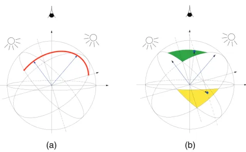
To solve Eq. (8), we only consider the set S of twice-lit unit-length normals n i.e., those where s1•n
>
0 and s2•n>
0. This set is an open part of Gaussian sphere G limited by two planes containing the origin (seeFig. 1a):( p1: s1 1n1+ s12n2+ s13n3= 0 p2: s2 1n1+ s22n2+ s23n3= 0 (9)
Planes p1 and p2 are orthogonal, respectively, to s1 and s2. At each twice-lit point (x, y) characterized by the graylevels I1(x, y) and I2(x, y), and by the supposedly known albedo q(x, y) 6= 0, system (8) admits two solutions, denoted n+(x, y) and n−(x, y), which are the intersections of S and of two planes which are obtained by trans-lating p1and p2of I1(x, y)
/
q(x, y) and I2(x, y)
/
q(x, y) in the directionsof s1and s2, respectively. SeeFig. 1b for a geometrical interpreta-tion of n+(x, y) and n−(x, y). The analytical formulae for them will be derived inSection 5.1. Let us denote by p the plane supported by s1 and s2and containing the origin of G. It is obvious that n+(x, y) and
n−(x, y) are symmetric with respect to p, for any (x, y) ∈ Y.
If I1(x, y) and I2(x, y) exactly match the Lambertian model (3), the non-differential problem (8) admits either two solutions, or one if
n+(x, y) = n−(x, y). But, if this model is not exactly satisfied, which may happen with real images, there may be some points (x, y) with-out any exact solution. The way to effectively handle these different cases will be specified inSection 5.1.
3.2. Differential formulations of the PS2 problem
Taking m = 2 in Eq. (7), and adding a Dirichlet boundary condi-tion, a first differential formulation of the PS2 problem is written as two nonlinear PDEs:
q(x, y)−˜s 1• ∇u(x,y)+s13 q 1+k∇u(x,y)k2 = I 1(x, y) a.e. (x, y) ∈ Y q(x, y)−˜s 2• ∇u(x,y)+s23 q 1+k∇u(x,y)k2 = I 2(x, y) a.e. (x, y) ∈ Y u(x, y) = g(x, y) ∀(x, y) ∈
∂
Y (10)Besides its nonlinearity, the main drawback of problem (10) con-cerns the need for a boundary condition: the function g(x, y), taken in the space of Lipschitz functions, represents a piece of information which is rarely available. On the other hand, since a common factor
q(x, y)
/
p1+ k ∇u(x, y)k2occurs in both PDEs of Eq. (10), we can com-bine them in order to simultaneously eliminate the albedo q(x, y) and the nonlinearity (we only have to suppose that q(x, y) 6= 0): hI2(x, y) ˜s1
− I1(x, y) ˜s2i•
∇u(x, y) = I2(x, y) s1
3− I1(x, y) s23 (11)
Considering the same boundary condition as in Eq. (10), we deduce:
( b(x, y)•∇u(x, y) = f (x, y) a.e. (x, y) ∈ Y u(x, y) = g(x, y) ∀(x, y) ∈
∂
Y (12) where: ( b(x, y) = I2(x, y) ˜s1− I1(x, y) ˜s2 f (x, y) = I2(x, y) s1 3− I1(x, y) s23 (13)This second differential formulation of the PS2 problem allows us to propagate boundary information g(x, y) across Y through vector
(b)
(a)
Fig. 1. (a) The setSof twice-lit normals, emphasized in red, is a part of Gaussian sphereGlimited by the planes p1and p2, which are orthogonal to light vectors s1and s2.
(b) An example where the system (8) admits two solutions in n (marked in red).
field b(x, y). Indeed, if b(x, y) and f(x, y) are two bounded (but not necessarily continuous) functions defined by Eq. (13), and if g(x, y) is a Lipschitz function, then Eq. (12) admits a unique Lipschitz solution
u(x, y)[15]. It is worth emphasizing that this implies that the differ-ential formulations of PS2 allow one to reconstruct surfaces that are differentiable almost everywhere. In practice, this means that sur-faces having sharp structures could be retrieved. In contrast, using the non-differential approach, the surface must be assumed to be C1, so that the normal is defined everywhere. If edges or depth disconti-nuities are in fact present, they must be adequately handled during the integration stage[13].
In order to ensure robustness to noise, propagation schemes used in [11]may be advantageously replaced by variational methods, recasting the linear PDE (12) as the following optimization problem:
min u: Y→R R R Y[b(x, y)•∇u(x, y) − f (x, y)] 2 dx dy s.t. u(x, y) = g(x, y), ∀(x, y) ∈
∂
Y (14)When m ≥ 3 images are available, it was shown in [31] that variational models such as Eq. (14) may be considered in several more difficult situations such as color PS, PS with pointwise sources or perspective PS, even without a boundary condition. Yet, when
m = 2, explicit knowledge of the function g is required in order to
ensure that the characteristics are not reconstructed independently. An alternative consists in using anisotropic regularization, in order to “couple” the 3D-reconstructions of the different characteristics, by ensuring smoothness along directions that are not tangent to the characteristics. A suitable variational model, which was introduced by Hernández et al. in[9], is written as follows:
min
u: Y→R
Z Z Y
n
[b(x, y)•∇u(x, y) − f (x, y)]2+ a1[b⊥(x, y)•∇u(x, y)]2
+a2£b⊥(x, y)⊤H(u)(x, y)b⊥(x, y) ¤2o
dxdy (15)
where the field b⊥ is perpendicular to the characteristic curves and H(u) is the Hessian matrix of u. The parameters a1 and a2
must be tuned appropriately, in order to ensure that the regu-larization is sufficient, yet avoiding over-smoothing the solution (cf.Section 5.4).
3.3. Example of PS2 problem
In order to question the consistency between the different for-mulations of the PS2 problem, let us take the example of a plane surface u(x, y) = x illuminated by light vectors s1 = [0, 0, 1]⊤and
s2 = 1 2 [1, 1,
√
2]⊤. If q ≡ 1, the images of this surface using Model (6) are uniform, with graylevels I1(x, y) =√1
2and I
2(x, y) = √2−1 2√2 . Let us first solve this PS2 example using the non-differential formulation (8), which is written as:
n3(x, y) =√1 2
n1(x,y)+n2(x,y)+√2 n3(x,y)
2 = √ 2−1 2√2 n1(x, y)2+ n2(x, y)2+ n3(x, y)2= 1 (16)
This system admits two solutions n+= √1
2 [−1, 0, 1]⊤and n−= 1
√
2[0, −1, 1]⊤, independently of (x, y). If the surface to be recon-structed is supposed to be differentiable everywhere, there are only two acceptable normal fields n(x, y) = n+or n(x, y) = n−. It follows from Eq. (4) that there are two possible values for ∇u(x, y):
−1 n+3(x, y) · n+ 1(x, y) n+ 2(x, y) ¸ =· 1 0 ¸ ; −1 n− 3(x, y) · n− 1(x, y) n− 2(x, y) ¸ =· 0 1 ¸ (17)
Imposing u(0, 0) = 0 to fix the integration constants, we finally obtain two solutions u+(x, y) = x and u−(x, y) = y. Fortunately, one of these solutions is the genuine surface.
Now, let us write the first differential formulation Eq. (10), sup-posing q ≡ 1: 1 q 1+k∇u(x,y)k2 = 1 √ 2 −∂xu(x,y)−∂yu(x,y)+√2 2 q 1+k∇u(x,y)k2 = √ 2−1 2√2 (18)
Note that no boundary condition is available. System (18) is equivalent to: (
∂
xu(x, y) +∂
yu(x, y) = 1 ° °∇u(x, y)°°2= 1 (19)By replacing k∇u(x, y) k2with
∂
xu(x, y)2+
∂
yu(x, y)2, we quicklyfind that Eq. (19) has the same solutions (17) in ∇u(x, y) as Eq. (16). Both formulations are thus consistent, in the sense that they provide the same global solutions.
It follows from the definitions (13) that:
b(x, y) = − 1
2√2[1, 1]
⊤ ; f (x, y) = − 1
2√2 (20)
In the absence of a boundary condition, the second differential formulation (12) reduces to:
∂
xu(x, y) +∂
yu(x, y) = 1 (21)Unsurprisingly, this PDE is the first equation of Eq. (19), which admits an infinity of solutions. For instance, all functions u(x, y) = a x + (1 − a)y + w(x − y), for any a ∈ R and any differentiable function
w : R → R, are solutions to Eq. (21). How can it be explained that this formulation does not lead to the same conclusion as the others? In fact, without a boundary condition, the differential formulation (12) is a necessary but insufficient condition. For better constraint, a boundary condition is required (but rarely available).
To conclude, there is obviously no inconsistency between the non-differential formulation and the first differential formulation of the PS2 problem. Hence, both these formulations should allow us to predict the same number of global solutions. Let us examine in more detail this issue.
4. PS2 problem: predicting the number of solutions
At any twice-lit point (x, y) ∈ Y, we know fromSection 3.1that the PS2 problem admits one or two solutions in n(x, y). Of course,
in order to predict the number of normal fields, the points where the normal can be determined unambiguously are of primary impor-tance. Such singular points have been studied in detail to solve the SFS problem[30].
4.1. Singular points
As already observed in Section 3.1, the first situation where normal uniqueness can be proved is reached when both solutions
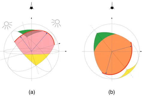
n+(x, y) and n−(x, y) to the problem (8) coincide. In this case, the unique solution is inside plane p. The set SRof such normals is a
geodesic on G. It is the intersection between S and p (seeFig. 2a). A second type of singular point occurs when one solution to Eq. (8) points towards the viewer (SGset inFig. 2b), while the other one
points away (SY set inFig. 2b). In this case, the ambiguities are
easy eliminated by choosing the “visible” normal. Let YR and YG
be the singular points sets where the normal belongs to SRor SG,
respectively.
Since a PS2 problem comes down to a pair of SFS problems (with the constraint that the camera pose is unique), one could wonder why the singular points of each SFS problem are not taken into account. These points are such that n = s1 in the first image, or
n = s2in the second. However, both these values of n are inside S
R,
since they support plane p. This shows us that the singular points of the PS2 problem include those of each SFS subproblem.
The normal field is continuous if the surface is supposed to be C1. Under such an assumption, is it possible to propagate the knowledge of the normal in a singular point to its non-singular neighbors? The answer to this question depends on which type of singular points is referred to. Let PR ∈ YRbe a singular point of the first type i.e., one
whose normal is inside SR. The normal in a non-singular neighbor ¯PR
of PRcan lie on both sides of SR. The subsets of S which are above and
below the geodesic SRare respectively called SUand SB, seeFig. 3.
In other words, there is a remaining ambiguity on the normal in ¯PR.
Now, let PG∈ YGbe a singular point of the second type, whose
nor-mal is inside SG. In any non-singular neighbor ¯PGof PG, we can infer
from the normal field continuity that the normal is inside SU. To
con-clude, the normal is unambiguously known in all points connected to
YGinside YrYR, which can be considered as supplementary singular
points.
(b)
(a)
Fig. 2. (a) Red geodesicSRis the intersection betweenSand p. Each normal pointing toSRis known without ambiguity. (b) This also holds true for each normal pointing toSG,
(b)
(a)
Fig. 3. (a) SetSBis colored in pink. It is the subset ofSbounded by equator E and geodesicSR. (b) Gaussian sphereGis seen from the camera point of view (i.e. z direction).
Orange setSUis the subset ofSlocated betweenSGandSR.
4.2. Using the singular points to construct a boundary condition
As an illustration, let us calculate a pair of images of the smooth surface depicted inFig. 4a, supposing q ≡ 1. The light directions are given, respectively, by (h1, 01) = (60◦, 17◦) and (h2, 02) = (135◦, 17◦), which avoids shadows (seeFig. 4b and c).
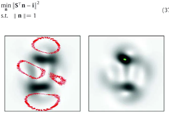
The sets of singular points YR and YG, which are numerically
estimated from the estimation of n+and n−described inSection 5, are superimposed to these images. In each of the five connected parts of YrYR, there are two solutions: one is contained in SU, the other in
SB. This gives rise to 25= 32 continuous normal fields. Nevertheless, a difference between our count and that put forward by Onn and Bruckstein[10]comes from the detection of YG: since the region
Y r YRcontaining YGis determined, only the other four regions are
ambiguous, leading eventually to 24= 16 possible normal fields. The solution u can be calculated over each connected singular points set, up to a constant of integration. Knowing that differen-tial formulation (12) needs a boundary condition to be well-posed, this is a simple way to construct one. Since
∂
Y is connected to YGinside Y r YR(seeFig. 4b and c), the solution can be univocally
cal-culated along
∂
Y. According to Mecca and Falcone[15], this allowsus to predict a unique solution, which is of course the original sur-face shown inFig. 4a. Based on this example, we could conclude that the non-differential and differential approaches to the PS2 resolu-tion are complementary, in order to predict the number of soluresolu-tions. Namely, the boundary condition required by the latter is provided by the former.
4.3. A possible remaining ambiguity
The conclusion of the previous section does not always hold true. For instance, in a case such as the example ofSection 3.3, there is no singular point (all the points have the same normal). Let us show another counterexample originally exhibited by Kozera in[32]. The surface represented by equation z = x y, with uniform albedo q ≡ 1, illuminated by light vectors s1 = [s, s, c]⊤ and s2 = [−s, −s, c]⊤, where s = √2
/
2 sin 0 and c = cos0, for a given 0 ∈]0, p/
2[, is characterized by the following graylevel functions: I1(x, y) =√s (−x−y)+c 1+x2+y2 I2(x, y) =−s (−x−y)+c√ 1+x2+y2 (22)
Fig. 4. (b–c) A pair of 256 × 256 synthetic images (stored in 32 bits) of the smooth surface (a), such that all the points are twice-lit, over which YR(in red) and YG(in green) are
The two first equations of the non-differential problem (8) are rewritten as: s [n1(x, y) + n2(x, y)] + c n3(x, y) =√s (−x−y)+c 1+x2+y2 −s [n1(x, y) + n2(x, y)] + c n3(x, y) =−s (−x−y)+c√ 1+x2+y2 (23)
Since by definition, s and c are nonzero, system (23) is equivalent to:
n1(x, y) + n2(x, y) =√1+x−x−y2+y2 n3(x, y) =√ 1 1+x2+y2 (24)
Using Eq. (24), the third equation of Eq. (8) can be rewritten as:
n1(x, y)2+ x + y p 1 + x2+ y2 n1(x, y) + x y 1 + x2+ y2 = 0 (25)
It is easy to check that this second-order equation always admits two real solutions in n1(x, y), which come down to a unique solution when y = x. These solutions give rise to two possible normals at each point (x, y) ∈ Y: n+(x, y) = 1 p 1 + x2+ y2 −y −x 1 ; n−(x, y) =p 1 1 + x2+ y2 −x −y 1 (26)
We deduce from Eqs. (26) and (4) two possible values for ∇u(x, y):
−1 n+ 3(x, y) · n+ 1(x, y) n+ 2(x, y) ¸ =· y x ¸ ; n−−1 3(x, y) · n− 1(x, y) n− 2(x, y) ¸ =· x y ¸ (27)
Both these vector fields are easily integrated, which provides us with two solutions u+(x, y) = x y and u−(x, y) = (x2 + y2)
/
2, up to two additive constants. That is to say, there is a remaining ambiguity.On the other hand, YG is empty, but it is easily deduced from
Eq. (26) that YRis the straight line y = x. The solution can therefore
be calculated along this line, up to a constant. Using a similar ratio-nale as inSection 4.2, we should conclude that the solution is unique, which would contradict the previous result. This contradiction is eas-ily explained: the prediction of Mecca and Falcone[15]holds true only if the solution is known on a curve which is not a characteristic. As we will see in the next section, this condition is precisely not valid in this case.
4.4. Using the characteristics to predict the number of solutions
In the previous example, each vector b(x, y) defined in Eq. (13) is parallel to [1, 1]⊤. The characteristics are thus the straight lines represented by equations y = x + g, g ∈ R, including the set YR.
Depth u can be univocally calculated along each characteristic, up to
a constant. This uniqueness result is not contradicted by the previous two-fold ambiguity since, for any g ∈ R:
u+(x, x + g) − u−(x, x + g) = x(x + g) −x2+
(
x + g)
2 2 = − g2 2 (28) is independent from x.If u(x, y) is known at one point of each characteristic, we have a better understanding why problem (12) has a unique solution. Fol-lowing this rationale, all functions of the folFol-lowing form seem to be solutions to the previous example:
u(x, y) = u+(x, y) + v( y − x) (29)
provided that v is a scalar function such that v(y − x) is constant along each characteristic. In fact, any function v is not acceptable because, as already noted, differential formulation (12) is a neces-sary but insufficient condition, in the absence of boundary condition. From Eq. (29), we deduce:
∇u(x, y) =· y − vx + v′′( y − x) ( y − x) ¸
(30)
Eq. (7) tells us that the surface z = u(x, y) of albedo q ≡ 1 is a solution to the previous example only if:
−s [ y−v′( y−x)]−s [x+v′( y−x)]+c
√
1+[ y−v′( y−x)]2+[x+v′( y−x)]2 = I
1(x, y)
s [ y−v′( y−x)]+s [x+v′( y−x)]+c
√
1+[ y−v′( y−x)]2+[x+v′( y−x)]2 = I
2(x, y) (31)
Using Eq. (22), we easily find the only two solutions in v′(y − x) to system (31): ( v′ 1( y − x) = 0 v′ 2( y − x) = y − x ⟹ ( v1( y − x) = K1, K1∈ R v2( y − x) =( y−x) 2 2 + K2, K2∈ R (32)
Plugging Eq. (32) into Eq. (29), we eventually obtain the two follow-ing solutions: ( u1(x, y) = u+(x, y) + K1 u2(x, y) = u+(x, y) +( y−x) 2 2 + K2= u−(x, y) + K2 (33)
This result confirms that there are only two analytical solutions u+ and u−, up to the constants K1and K2.
4.5. Integrability constraint
Even if vector field [p, q]⊤ = [−n1
/
n3, −n2/
n3]⊤is easily calcu-lated from a normal field, there is no guarantee that this vector field is integrable i.e., that it satisfies the integrability constraint[33]:∂
p∂
y=∂
q∂
x (34)whereas this is required, if the surface is supposed to be at least C2, in order to be sure that equation ∇u = [p, q]⊤has a solution in u. Onn and Bruckstein note in[10]that “most of the time”, in each con-nected part P of YrYR, one of the two possible normal fields may be
discarded since it is not integrable. To decide, they rely on a criterion deduced from Eq. (34):
Z Z (x,y)∈P ·
∂
p∂
y(x, y) −∂
q∂
x(x, y) ¸2 dx dy = 0 (35)They also characterize the “rare cases” where Eq. (35) is satisfied by more than one normal field, in which case the PS2 problem admits several solutions. In fact, the examples ofSections 3.3 and 4.3are such “rare cases”.
Let us now return to the example of Fig. 4. Using the non-differential formulation, we found 24 = 16 possible normal fields. A more complex rationale based on the topology of sets YRand YG
allowed us to predict a unique solution. Consequently, among the sixteen normal fields, only one is integrable. However, a prediction based on topology is difficult to extend to the discrete framework, since the notion of continuity will be lost.
Indeed, let us calculate the sets YRand YGwhen the images are
quantized. It is clear fromFig. 5that the topology of YRis very
sen-sitive to quantization noise. It is thus no longer possible to predict the number of solutions using the rationale ofSection 4.2from such a fragmented set YR.
We show in the next section that it is possible to efficiently find the most integrable normal field, and hence to eliminate the ambiguities of the PS2 problem, without knowledge of a boundary condition[11]nor parameter tuning[9].
5. Photometric stereo using two images: a numerical resolution
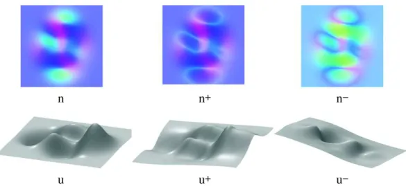
We know fromSection 3.1that the PS2 problem admits at most two solutions in n at each point (x, y) ∈ Y (seeFig. 6). We can thus a priori construct at most 2|Y|different discrete normal fields, where |Y| denotes the number of pixels inside Y. Yet, except in some rare cases[10], only one of these candidates is integrable. Let us show how to efficiently find this most integrable normal field.
5.1. Estimating the candidate normal fields
Problem (8) has two solutions n+and n−at each point. Let us first show how to express these solutions using a purely algebraic method.
At each point (x, y) ∈ Y, the two first equations of problem (8) write (the dependencies in (x, y) are omitted):
· s1⊤ s2⊤ ¸ | {z } S⊤∈R2×3 n = "I1 q I2 q # | {z } i∈R2 (36)
With a view to solving Eq. (36) in the least-squares sense in order to handle quantization noise, we reformulate problem (8) as follows:
min n ° °S⊤n − i°°2 s.t. k n k= 1 (37)
Fig. 5. Two same images as inFig. 4, quantized using 256 levels (8 bits). While this is
not the case of YG(right), YRbecomes fragmented (left).
The singular value decomposition (SVD) of S⊤can be written as:
S⊤= USV⊤= s1u1v⊤
1 + s2u2v⊤2 (38)
In Eq. (38), s1 ≥ s2
>
0 are the pair of strictly positive singular values of S (S has rank 2, since s1and s2are non-collinear), u1and u2 are orthonormal vectors of R2, and v
1and v2are orthonormal vectors of R3. It can be shown (Theorem 5.5.1 in[34]) that the minimum-norm solution of the least-squares problem resulting from Eq. (36): n0= arg min n∈E k n k s.t. E =©n ∈ R3, k S⊤n − ik2≤k S⊤m − ik2∀m ∈ R3ª (39) is written as: n0= u⊤ 1i s1 v1+ u⊤ 2i s2 v2 (40)
Let us now solve problem (37). Three cases can occur:
1. If kn0k = 1, then n+ = n− = n0is the only solution to Eq. (37), and the objective is null. This corresponds to the singular points in YR, cf.Section 4.1.
2. If kn0k
<
1, then neglecting the unit-length constraint, there exists a set of solutions with null objective to the optimiza-tion problem (37), which is written as:n0+ Rv3 (41)
where v3is a unit-length vector of the kernel of S⊤(this ker-nel has dimension 1, according to the rank theorem). Two of these solutions have unit-length, which are the only two solutions to problem (37)2: ( n+= n 0+ p 1− kn0k2v3 n−= n0−p1− kn0k2v 3 (42)
3. Finally, if kn0k
>
1, there is no solution with null objective to problem (37). It is tempting to choose the approximate solution n+= n−= n0kn0k, but this is not the real solution to Eq. (37). It is proven in[34]that this solution writes as:
n(k0) = s1u⊤1i s12+ k0 v1+ s2u⊤2i s22+ k0 v2 (43)
which reduces to n0when k0= 0, yet k0is in fact the unique positive solution in k to the following secular equation:
à s1u⊤1i s12+ k !2 + à s2u⊤2i s22+ k !2 − 1 = 0 (44)
Eq. (44) could be rewritten under the form of an algebraic equation of degree 4 in k, and solved using the Ferrari– Cardan formulae. Instead, we used in our implementation a Newton method. However, it should be reminded that an equation of this type has to be solved at each pixel such that kn0k
>
1. If the targetted application has real-time require-ments[16], n0/
kn0k may be preferred as a fast approxima-tion of the soluapproxima-tion to Eq. (37), although it is not the exact solution.2 The expressions in Eq. (42) a posteriori explain the signification of the superscripts
n
+
n
n
−
u
+
u
u
−
Fig. 6. Top: RGB-encoded normal fields (n is the ground truth, n+and n−are the normal fields estimated by Eq. (42)), using the quantized dataset presented inFig. 5. Bottom:
3D-shapes obtained integrating the normals[13]. The normal fields n+and n−are only two solutions among 2|Y|, since any combination of both these normal fields is also
plausible.
5.2. Disambiguating the problem by graph cut
The case kn0k
<
1 being by far the most frequent, we can actually build almost 2|Y|normal fields, which are all solutions to problem (8). In[35], it is proposed to better constrain the problem assuming that the normals are distributed according to a Laplace law, but this assumption is hard to justify. As discussed inSection 4.5, we would rather advise using the integrability constraint of the normal field, which is much less restrictive (the surface is simply assumed C2, at least piecewise). We will now describe the practical resolution of the problem (8) based on this constraint.Finding the “most integrable” normal field amounts to finding the one such that the integrability constraint (34) is “best” approximated over Y. This can be formulated as the variational problem (35).
Yet, such a variational problem does not account for the fact that we know explicitly the 2|Y|possible normal fields. An exhaustive search of the most integrable normal field could be preferred, but it may be computationally infeasible on large data. Instead, we sug-gest to recast the task of finding the most integrable normal field as a binary labeling problem whose solution can be found efficiently, by means of the graph cut algorithm[12].
Let us attribute to each pixel a label l ∈ {+, −} indicating the nor-mal n+or n−, and let us denote byhpl, qli⊤= h−nl
1
/
nl3, −nl2/
nl3 i⊤ the corresponding discrete approximation of the surface gradient ∇u. The “optimal” labeling l : Y → {+, −} is the one which makes the normal field the “most integrable”. Thus, we now have to solve the following discrete version of the variational problem (35) over Y:min l X X (x,y)∈Y "
∂
pl∂
y(x, y) −∂
ql∂
x(x, y) #2 (45)In order to discretize the space derivatives of problem (45) using finite differences of order 1, we should consider the four possible
cliques families of order 3:
C13=©©(x, y), (x − 1, y), (x, y − 1)ª∈ Y3ª C23=©©(x, y), (x + 1, y), (x, y − 1)ª ∈ Y3ª C33=©©(x, y), (x − 1, y), (x, y + 1)ª ∈ Y3ª C43=©©(x, y), (x + 1, y), (x, y + 1)ª ∈ Y3ª (46)
If we denote (l1, l2, l3) the labels of each clique’s three pixels, in the same order they are defined in Eq. (46), problem (45) can be rewritten as: min l X c3 ∈C3 Vint c3(l1, l2, l3) (47) where C3= ∪4
i=1Ci3, and potential Vcint3(l1, l2, l3) gives the local integra-bility for the current clique c3and the current labeling l. For example, if c3 1∈ C13: Vint c3 1 (l1, l2, l3) = h³ pl1(x, y) − pl3(x, y − 1)´−³ql1(x, y) − ql2(x − 1, y)´i2 (48)
Problem (47) is a labeling problem where the local potential depends on the current pixel and on two of its neighbors. Such com-binatorial optimization problems have been studied in[36], where it has been proven that the graph cut algorithm[12]can be used to minimize the energyPc3
∈C3Vcint3(l1, l2, l3), provided that its regularity
(sub-modularity) is ensured, which means here:
Vint
c3(+, +, l3) + Vcint3(−, −, l3) ≤ Vcint3(+, −, l3) + Vcint3(−, +, l3) Vint
c3(+, l2, +) + Vcint3(−, l2, −) ≤ Vcint3(+, l2, −) + Vcint3(−, l2, +) Vint
c3(l1, +, +) + Vcint3(l1, −, −) ≤ Vcint3(l1, +, −) + Vcint3(l1, −, +) (49)
for any c3 ∈ C3 and any (l
1, l2, l3) ∈ {+, −}3. Of course, these inequalities have no reason to be satisfied.
5.3. Ensuring the regularity condition
To ensure the regularity condition, we modify the problem (47) by introducing a regularization term of the Ising type:
min l X c3∈C3 Vcint3(l1, l2, l3) + X c2∈C2 VIsingc2 (l1, l2) (50)
where C2 = ∪4
i=1Ci2 gathers the four following sets of cliques of
order 2: C12=©©(x, y), (x − 1, y)ª∈ Y2ª C22=©©(x, y), (x, y − 1)ª∈ Y2ª C32=©©(x, y), (x − 1, y − 1)ª ∈ Y2ª C42=©©(x, y), (x + 1, y − 1)ª ∈ Y2ª (51)
and VIsingc2 (l1, l2) is defined as follows, where (l1, l2) denote the labels
of the two pixels of each clique c2∈ C2, in the same order they are defined in (51):
VcIsing2 (l1, l2) = bc2 d(l16= l2) (52)
In Eq. (52), bc2 is a positive or zero local coefficient i.e., such a
coefficient must be fixed for each c2 ∈ C2. Enforcing the regularity condition for Eq. (50), we deduce a lower bound for each bc2. For
example, if c2 3=©(x, y), (x − 1, y − 1)ª ∈ C32: bc2 3≥ 1 2 max ( 0, max (l3,l4)∈{+,−}2 ½ DVcint3 3 (l3), DVcint3 2 (l4) ¾) (53) where c3
3= c23∪ (x, y − 1), c32= c23∪ (x − 1, y) , and (l3, l4) denote the labels of (x, y − 1) and (x − 1, y), respectively. Finally, for j ∈ {2, 3} and
k ∈ {+, −}: DVcint3 j (k) = Vint c3 j (k, +, +) + Vint c3 j (k, −, −) − V int c3 j (k, +, −) − V int c3 j (k, −, +) (54)
From a Markovian point of view, our approach consists in using non-stationary Ising models. The use of such models corresponds to a piecewise uniform prior on the labeling l. We know fromSection 4 that there exist a finite number of connected areas over which the solutions n+and n−are different (these areas are bounded by the set YR). If these normal fields are estimated as indicated inSection 5.1,
they will be continuous inside each area, so the optimal labeling should change only along their boundaries. The Ising prior is thus consistent with the theoretical analysis conducted inSection 4.
Yet, in order not to bias the 3D-reconstruction which should rather be guided by integrability, this prior should have as little influence as possible: according to inequalities like Eq. (53), it is possible to predict, for each clique c2 ∈ C2, the smallest value of coefficient bc2 to ensure the regularity condition. These
coeffi-cients should therefore not be considered as parameters, which is an advantage. This allows us to limit the energy regularization, only in order to ensure regularity in the sense of Kolmogorov[36], thus avoiding oversmoothing. When coefficients bc2are not fixed to their
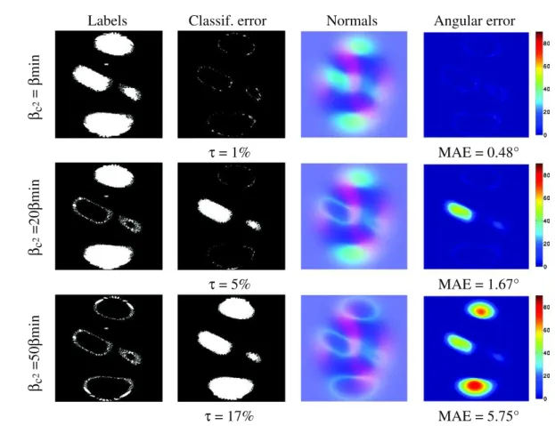
Labels
Classif. error
Normals
Angular error
β
c
2=
β
min
τ = 1%
MAE = 0.48°
β
c
2=20
β
min
τ = 5%
MAE = 1.67°
β
c
2=50
β
min
τ = 17%
MAE = 5.75°
Fig. 7. The oversmoothing of the labeling obtained using high values of coefficients bc2, on the dataset fromFig. 6. From left to right: obtained labeling (black for n+, white for
n−), XOR map between the estimated labels and the ground truth one (t indicates the percentage of wrong labels), estimated normal field, and absolute angular error in degrees (MAE is the mean angular error). The choice bc2= bminindicates minimal coefficients (cf. Eq. (53)).
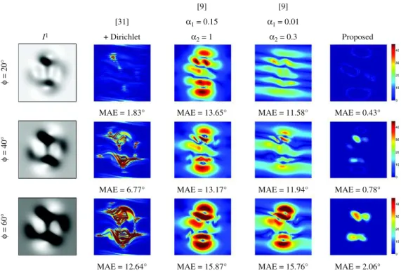
[9] [9] [31] α1 = 0.15 α1 = 0.01 I1 + Dirichlet α 2 = 1 α2 = 0.3 Proposed φ = 20°
MAE = 1.83° MAE = 13.65° MAE = 11.58° MAE = 0.43°
φ
= 40°
MAE = 6.77° MAE = 13.17° MAE = 11.94° MAE = 0.78°
φ
= 60°
MAE = 12.64° MAE = 15.87° MAE = 15.76° MAE = 2.06°
Fig. 8. Angular errors on the normals. The dataset fromFig. 5was considered while increasing the zenithal angles 0 for the lightings, in order to create stronger shadowing effects.
Our method confines the errors in the shadow areas, while requiring neither a boundary condition nor parameter tuning (a1and a2are defined in Eq. (15)).
minimum values, the labeling is oversmoothed, which biases the 3D-reconstruction (seeFig. 7). Our approach thus avoids the difficulty of tuning the regularization parameters, which is a problem with existing methods (cf.Figs. 8 and 9).
5.4. An efficient method for solving the PS2 problem
To sum up, the method of resolution of the PS2 problem that we recommend comprises two stages:
1. The calculation of normal fields n+ and n− as indicated in Section 5.1.
2. The disambiguation of the problem using the integrability cri-terion, an 8-connected Ising model, the minimum values of the coefficients bc2 like for instance Eq. (53), and the graph cut
algorithm.
Both steps can be efficiently conducted: the initial solutions n+ and n−are explicit, and optimization by graph cut is very efficient3.
The 3D-reconstruction shown in the first row ofFig. 7is obtained applying this method to the example ofFig. 6. The normal field is very similar to that of the ground truth: when the albedo is known and in the absence of shadow, our method is able to recover almost exactly the genuine normals.
In addition to being parameter-free and not requiring a boundary condition,Figs. 8 and 9show us that the proposed method is able to confine estimation errors, which may be useful if a shadow is present in one (or both) of the images. This is in contrast with existing meth-ods, for which an estimation error in one pixel may propagate to its neighbors.
Yet, our approach has one major weakness with respect to exist-ing methods. Indeed, we assume that the albedo is known. In contrast, since existing methods[9,31]are based on image ratios, knowledge of the albedo is not required. As a consequence, their
3 It is stated in[12]that “the running time is nearly linear in practice”.
methods are robust to unpredicted albedo variations, while ours is not. As it is illustrated inFigs. 10 and 11, this represents an impor-tant limitation of our method. To conclude, our method yields overall more accurate 3D-reconstructions than existing ones, and is more flexible (neither need for boundary condition nor parameter tuning), but only when the albedo is known. This restriction is also recurrent in shape-from-shading, where albedo estimation must be carried out beforehand using interpolation techniques[37,38], or within the 3D-reconstruction process by introducing priors on the albedo and the shape[39].
For sake of completeness, well-posedness of the PS2 problem with unknown albedo is briefly discussed hereafter.
5.5. PS2 problem with unknown albedo
At this stage, it is interesting to quote a variant of the PS2 problem, where the surface to be reconstructed has an unknown albedo. The presence of a supplementary unknown q(x, y) at each point (x, y) ∈ Y could drastically complicate the problem. A main feature of the PS3 problem is that the albedo can be univocally estimated[6]. This is not the case for SFS since, even if the albedo is known, the problem
[31] + Dirichlet [9] (α1 = 0.15, α2 = 1)
[9] (α1 = 0.01, α2 = 0.3) Proposed
[9] [9] [31] α1 = 0.15 α1 =0.01 I1 + Dirichlet α 2 = 1 α2 =0.3 Proposed d = 10
MAE = 1.88º MAE = 14.06º MAE = 11.82º MAE = 2.71º
d
= 50
MAE = 2.00º MAE = 14.16º MAE = 11.87º MAE = 9.22º
d
= 100
MAE = 2.05º MAE = 14.24º MAE = 11.89º MAE = 14.50º
ρ
ρ
ρ
Fig. 10. The 256 × 256 images were created with q everywhere equal to 1 except on a diagonal band with width dqpixels where it was set to 0.9. Assuming (wrongly) that q ≡ 1
induces a bias with our method, while existing methods are independent from the albedo.
is usually ill-posed[40]. We will see that the PS2 problem with unknown albedo is more similar to SFS than to PS3.
Let us first give a geometric interpretation of Eq. (11). Since s = £˜s⊤, s3¤⊤ and n(x, y) is parallel to [−∇u(x, y)⊤, 1]⊤, this equation is rewritten as:
h
I2(x, y) s1
− I1(x, y) s2i•n(x, y) = 0 (55)
Eq. (55) can be directly derived from the two first equations of Eq. (8). It means that n(x, y) lies within a plane w(x, y) which is orthogonal to the vector I2(x, y)s1− I1(x, y)s2. Naturally, w(x, y) is orthogonal to the plane p as well, which is supported by the vectors
s1and s2. It is noteworthy that Eq. (55) holds true for any albedo value q(x, y), because Eq. (11) has been derived from problem (10) by elimination of q(x, y).
We know from Section 3.1 that, for any known albedo value
q(x, y), problem (8) has two solutions n+(x, y) and n−(x, y) which are symmetric with respect to p. The geometric interpretation of
[31] + Dirichlet [9] (α1 = 0.15, α2 = 1)
[9] (α1 = 0.01, α2 = 0.3) Proposed
Fig. 11. 3D-reconstructions corresponding to the second row inFig. 10.
Eq. (55) means that for a fixed pair of graylevels (I1(x, y), I2(x, y)), dif-ferent values of q(x, y) will provide difdif-ferent values of n+(x, y) and
n−(x, y) which all lie within w(x, y).Fig. 12shows us that n+(x, y) and
n−(x, y) move towards plane p as q(x, y) decreases from 1 towards a limit value qinf(x, y) which corresponds to the limit case n+(x, y) =
n−(x, y). Hence, at each (x, y), a range of values [qinf(x, y), 1] are fea-sible for q(x, y). If s1 6= s2, it can be shown that this limit is:
qinf(x, y) = s
I1(x, y)2+ I2(x, y)2− 2 I1(x, y) I2(x, y) (s1•s2)
1 − (s1•s2)2 (56)
Hence, the PS2 problem with unknown albedo is ill-posed. How-ever, it is worth underlining that, when a boundary condition is available, problem (12) can be solved without any knowledge of
q(x, y). Moreover, q(x, y) can be a posteriori calculated in this case,
using any of the PDEs of Eq. (10).
Fig. 12. Normals n+(x, y) and n−(x, y) move towards p as q(x, y) decreases from 1
towards a minimum value qinf(x, y) which corresponds to the limit case n+(x, y) = n−(x, y).
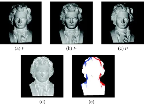
(a)
I
1(b)
I
2(c)
I
3(e)
(d)
Fig. 13. (a–b–c) Three photographs of a plaster bust of Beethoven. (d) Albedo estimated using the PS3 technique, which is biased in the shadow areas. (e) Partition of Y: Y3
(white), Y1,2
2 (red), and Y 2,3
2 (blue). PS2 is applied in the Y2sets, and PS3 elsewhere.
As an example, let us reconsider the example ofSection 3.3, under the assumption that q(x, y) is unknown. The non-differential problem (16) becomes: q(x, y) n3(x, y) =√12 q(x, y) n1(x,y)+n2(x,y)+ √ 2 n3(x,y) 2 = √ 2−1 2√2 n1(x, y)2+ n2(x, y)2+ n3(x, y)2 = 1 (57)
For any given value of q(x, y), the two first equations of Eq. (57), which can be rewritten as n3(x, y) =√ 1
2 q(x,y)and n1(x, y) + n2(x, y) = −1
√2 q(x,y), admit an infinity of solutions:
n(x, y) = 1 q(x, y) 1 √ 2 −1 0 1 + t −1 1 0 (58)
which depend on a real parameter t. Replacing the expression (58) of n(x, y) in the third equation of Eq. (57), we find after some algebra the following result:
n(x, y) = 1 2√2 q(x, y) −1 − 4p4 q(x, y)2− 3 −1 + 4p4 q(x, y)2− 3 2 (59)
where 4 = ±1. In Eq. (59), the albedo value q(x, y) can be arbitrar-ily chosen, provided that 4q(x, y)2− 3 ≥ 0. This means that q(x, y) ≥ √
3
/
2, which is actually the limit value qinf(x, y) given in Eq. (56). Clearly, this problem is ill-posed since at each point (x, y) ∈ Y, for each value q(x, y) ∈ h√3/
2, 1i, there are two possible normals, due to the two possible values of 4 in Eq. (59).To conclude, with the non-differential approach that we follow in this article, the PS2 problem can be solved unambiguously only if the albedo is known beforehand. Nevertheless, let us now show that solving the PS2 problem in an efficient way is not a purely formal challenge.
6. An application: improving three-source photometric stereo
We have seen in Section 5 that the accuracy of PS2 strongly depends on the presence of shadows. The simplest way to ensure robustness to shadows is to consider a third image, i.e. the PS3 problem. By placing the lights appropriately, one can ensure that each surface point is lit in at least two out of the three images, and resort to a combination of the PS2 and the PS3 techniques. This can improve a lot the accuracy of real-time PS based on color photometric stereo[16].
6.1. The recurrent problem of shadows
The three photographs of the first row ofFig. 13, which are avail-able on the web4, show a plaster bust of Beethoven illuminated by
three non-coplanar, parallel and uniform light beams. Since the light vectors are provided, these real data are particularly well adapted to the PS3 technique (seeSection 2.2). In addition, let us remark that no boundary condition is available.
Solving at each point (x, y) ∈ Y a linear system of type (6), then integrating the normals using [13], we indeed obtain a “satisfac-tory” 3D-shape (seeFig. 14), but this is contradicted by the estimated albedo (seeFig. 13d), which should be uniform since the material is homogeneous. We also note that the points where the albedo estimate is biased lie inside the shadows.
The problem of dealing with shadows in PS is well-known. Because they constitute an unavoidable departure from the Lamber-tian model (2), shadow graylevels are usually considered as outliers. In this view, most contributions[24–29]assume that m
>
3 images are available, which is not the case here. Only[9]considers the casem = 3, and thus “two-source photometric stereo [. . . ] in the presence
of shadows”.
Based on a simple shadow detection (we used the same graph cut-based approach as in[41]),Fig. 13e shows how Y can be split into
PS3
PS2
PS3/PS2 ([9])
PS3/PS2 (ours)
Fig. 14. 3D-shape reconstructed from the three photographs of the top line ofFig. 13, using different techniques. The PS2 technique is applied to the pair of images (I1, I2).
four subsets: Y3, Y1,22 , Y1,32 and Y2,32 , with straightforward notations (Y1,32 is empty in this example). A PS3
/
PS2 combination can then be considered: the PS2 technique can be used over the pixels lit in only two images, and the PS3 technique elsewhere. The PS3 solution is also used for the points shadowed in more than one image, for sta-bility reasons, yet it would probably be possible to define three other subsets Y11, Y21and Y31and resort to SFS over these sets.
To apply the method described inSection 5.4to the PS3
/
PS2 com-bination, we first need to estimate the albedo. Knowing that it is uniform since the material is homogeneous, this can be carried out by evaluating the histogram peak of the estimated albedo inside the set Y3, which can be considered as the “real” albedo: we obtained the value q = 0.
74.As shown inFig. 14, using only two images yields biased results because PS2 is not robust to shadows. Yet, as shown inFig. 15, com-bining the PS3 and PS2 techniques can improve a lot the accuracy
of the 3D-reconstruction. In addition, it seems that using the pro-posed PS2 framework inside this combination improves the results, in comparison with state-of-the-art.
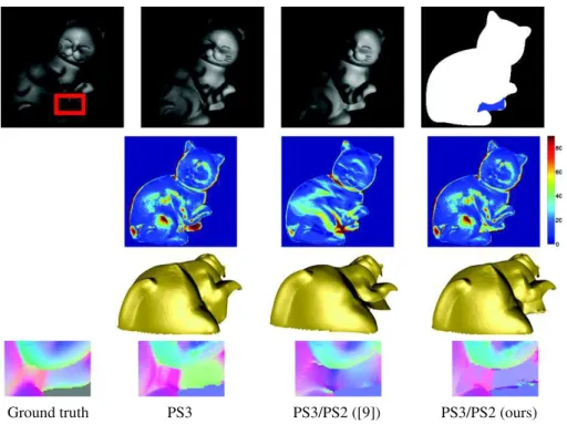
In order to quantitatively assess the accuracy of the proposed PS2 framework, we extracted three images from the dataset[42], which contains 96 images in total, and for which ground truth normals are available. As shown inFig. 16, our PS2 method was applied only over a shadow area, indicated in red, where the albedo is approximately uniform. The proposed method is able to handle shadows even when they are located near the boundaries, which is a known failure case of the differential approach in the absence of a boundary condition[9].
6.2. Color photometric stereo
Hernández et al. argue the following in [9]: “Using photomet-ric stereo on just three images may seem like an unreasonably hard
PS3
PS3/PS2 ([9])
PS3/PS2 (ours)
Fig. 15. Frontal (top) and side (bottom) views of the 3D-reconstructions obtained using PS3, and two versions of the combination PS3/PS2. Ours is able to recover fine-scale details
Ground truth
PS3
PS3/PS2 ([9])
PS3/PS2 (ours)
Fig. 16. First row: three images of a Lambertian object, and the Y3/Y2,32 partition. The area indicated in red lies almost entirely in the shadow in the first image. Second row:
angular error (in degrees) obtained using, from left to right, the PS3 method (MAE = 11.84◦), the PS2/PS3 combination from[9](MAE = 11.27◦), and the proposed one MAE = 11.57◦). The differential approach, which ensures smoothness, is globally more satisfactory than the non-differential one. Third row: 3D-reconstruction results. Fourth row: close-up on the estimated normals over the area indicated in red. The MAE are, respectively, 20.79◦, 25.49◦and 16.73◦. Our method achieves the best 3D-reconstruction in the shadow area.
Fig. 17. (a) An RGB image of a face illuminated by three directional, non-coplanar, color light sources. (b–c–d) Decomposition of the image (a) in three channels (red, green, blue).
(e) Partition of Y into sets Y3(white), YR,B2 (green), and YG,B2 (blue).
restriction. There is, however, a particular situation when only three images are available. This technique is known as color photomet-ric stereo”. Indeed, the most straightforward application of PS2 is color photometric stereo, a technique where three light sources with different colors and positions are used to simultaneously pro-vide three (graylevel) images of the surface under three different illuminations.
This idea is due to Kontsevich et al., who show in[43]how to reconstruct the 3D-shape of a white painted scene, illuminated by
m = 3 color light sources. Indeed, the number of channels of a
stan-dard color image is three. Considering each channel as a graylevel image, a single RGB image is enough to apply the PS3 technique. A deformable scene such as a face can therefore be reconstructed, even if the person is not standing still: Hernández et al. show in[16]“how multispectral lighting allows one to essentially capture three images (each with a different light direction) in a single snapshot, thus mak-ing per-frame photometric reconstruction possible”. An example of
such an RGB image extracted from a video sequence5is shown in
Fig. 17. Let us nevertheless point out that the albedo map should be the same in each channel. In practice, this requires that the scene is made-up. Since applying make-up also ensures that the albedo is uniform, it can be estimated by evaluating the histogram peak.
We can apply the PS3 technique to the image ofFig. 17a but, with-out any specific treatment, the result is biased around the nose (see Fig. 18), since the shadow renders the red channel unusable in this area (seeFig. 17b).
As inSection 6.1, the histogram of the albedo allows us to esti-mate the (uniform) albedo, and therefore to use the PS2 framework within the PS3