Contribution récente des glaciers des Andes à la ressource en eau et à la hausse du niveau marin. Apport des observations satellitaires

(1)

THÈSE

En vue de l’obtention du

DOCTORAT DE L’UNIVERSITÉ DE TOULOUSE

Délivré par l'Université Toulouse 3 - Paul Sabatier

Présentée et soutenue par

Inés DUSSAILLANT

Le 11 octobre 2019

Contribution récente des glaciers des Andes à la ressource en

eau et à la hausse du niveau marin. Apport des observations

satellitaires

Ecole doctorale : SDU2E - Sciences de l'Univers, de l'Environnement et de

l'Espace

Spécialité : Océan, Atmosphère, Climat

Unité de recherche :

LEGOS - Laboratoire d'Etudes en Géophysique et Océanographie Spatiale

Thèse dirigée par

Etienne BERTHIER et Vincent FAVIER

Jury

M. Christophe KINNARD, Rapporteur M. Daniel FARINOTTI, Rapporteur Mme Dana FLORICIOIU, Examinatrice

M. Vincent JOMELLI, Examinateur M. Etienne BERTHIER, Directeur de thèse

(2)

In every walk with Nature one receives far more than he seeks

(3)

It was walking through this exact glacial landscape when I decided to study glaciers and pursue my career as a glaciologist. So, first of all, I have to thank Nature and this particular moment for providing me the clarity needed to take an important decision.

I happened to end in France doing the project that I most dreamt of: measure the recent evolution of Andean glaciers (including the glaciers in the picture!). For this opportunity and for believing in me, I thank Etienne Berthier, my thesis Director. A Director of excellence. Always available, always honest with his constructive critics and emphasising on RIGOR!. It was a privilege to work at his side and to learn the ways of science from his good example, in line with my own principles. The best way of thanking him is to be able to pass forward all the knowledge he gave to me! That is my goal and he is the example to follow.

For being welcomed at the birthplace of glaciology in France (IGE) I thank Vincent Favier, my Co-director. His never-ending ideas where always motivating, it was only a pity to have a deadline to finish my contract!

Only a good leader knows how to choose and build a good team: I am proud to have formed part of the ASTERIX family during this last three years. I thank Fanny for her never-ending will to help and to be available for everything. Full of positive energy and motivation for science and mountains, she became an inspiring friend. Romain came later bringing the dynamism of the ASTERIX team to its tipping point. Thanks to him -also and inspiring friend and colleague- for all his help, all his patient explanations and for his infinite kindness.

(4)

Acknowledgements

of my thesis. And Antoine, for his important contribution on the Tropics. I also thank my colleagues from Argentina Mariano, Pierre y Lucas, that always received me with the arms wide open. Salud! for all the good –and bad- experiences in the field, the asados and the scientific discussions. And for more to come!. Also thanks to Hernan, Lidia, Laura, Pepe, Ricardo, Cristi and the un-nameable amount of friends and colleagues from Mendoza.

For all the "PhD moments", all those tears spread, the hugs, and then the laughs out loud when we where supposed to be quiet, I thank Violaine! Our office was full of good energy -and full of plants- It was a pleasure to share it with her and share this bitter-sweet-process together. Thanks to all the team of PhD’s and Post-Docs in LEGOS and more; my good friend Marina (the unidentified poet), Cesar (in his deep heart he knows he is a climber), Joaquin, Antoine, Fifi, Marine, Zaida, Audrey, Manon, Lise, Alice, Simon, Carlos y Cami. And from IGE, all the good friends and master fellows that continued in science Gabi (amigas desde la Patagonia hasta siempre!), Marion (very important at the end, she knows why), Maria, Lucas and Marion, Jay, and el chilenito Claudio! Thank also to all the people behind this two laboratories, helping science to move forward: the Directors -Alex and Pierre-, the beautiful and efficient secretaries -Agathe, Nadine, Martine and Brigitte-, the informatics and all the permanent re-searchers that create this motivating environments. A special thanks to the members of the ECHOS team -Frederique, Sarah, Alejandro, Denis, Sylvain, Alexei- for the glacio-coffees shared and the smiles crossing corridors.

From the rest of the Toulousain world I thank Thomas who was always there with his bike, was it for a good climb or just a talk. Harold and Cony arrived in the most important moment to remind me the taste of my longed Chile. But the most special embrace goes to my best yoga teacher and friend from the heart Gerda and the always smiling and caring Marcos. Mamita y Papito -and Luna of course-, the closest to a family I had in France. They showed me the secrets of Ariège on top of skis, with climbing shoes or without them. Their kindness and care kept me going through the most difficult parts of this journey. Thanks to la Payasita Caro, my deep friend and coach -of body and soul-, even from far away she managed to make me laugh and sweat (and allowed my ass not to go square while writing this the-sis). Thanks also to Chris, for sharing this short moment of life with me.

My real family from far away stayed always a strong support. Thanks to my sisters, nephews and nieces, for their loving messages. But specially to my parents, if it wasn’t for their effort, I would never had the chance to be -here, in this moment- and become the glaciologist I dreamed of while walking over my glaciers.

(5)

Les glaciers Andins présentent des taux de recul parmi les plus important au monde, et contribuent à la hausse du niveau des mers. Ils constituent aussi des ressources en eau vitales pour les vastes zones semi-arides le long de la Cordillère des Andes (10°N-56°S), en alimentant les rivières lors des sécheresses. En dépit du retrait des glaciers Andins, les mesures directes des fluctuations glaciaires sont éparses, de court terme, incomplètes, et ne permettent donc pas une estimation précise de la perte de glace récente à l’échelle de la chaîne entière. Décrire quantitativement cette perte à différentes échelles spatio-temporelle est cruciale afin de mieux anticiper les impacts écologiques, économiques et sociaux. Premièrement, nous avons évalué la performance d’une méthode visant à calculer les changements de masse des glaciers Andins. Cette méthode utilise les séries temporelles des modèles numériques de terrain (DEM) produit par des images stéréoscopiques Advanced Spaceborn Thermal Emission and Reflection Radiometer (ASTER). Sur la zone de validation de la méthode, le Champ de Glace Nord de Patagonie (NPI), nous avons observé un bilan de masse fortement négatif de -1.06 ± 0.14 m w.e. a−1pour la période 2000-2012. Ces résultats sont cohérent avec les estimations faites précédemment, mais aussi avec une seconde estimation (-1.02 ± 0.21 m w.e. a−1) obtenue indépendamment par différentiation de DEMs de meilleur résolution, Shuttle Radar Topography Mission (SRTM) et Satellite pour l’Observation de la Terre 5 (SPOT5). Ce travail nous a permis de (i) valider la méthode appelée « ASTER monitoring Ice towards eXtinction » (ASTERIX) sur la totalité des Andes, (ii) confirmer l’absence de pénétration du signal radar SRTM dans la bande C sur la neige du NPI (sauf pour une petite région au dessus de 2900 m a.s.l) avec des effets négligeables sur le bilan de masse du NPI; et enfin (iii) fournir la base de travail pour une analyse des variations du bilan de masse du NPI durant différentes sous périodes entre 1975 et 2016, grâce à des DEMs supplémentaires.

Ensuite, nous avons généré plus de 30000 DEMs ASTER afin de calculer la perte de l’intégralité des glaciers Andins, et ce pour les deux dernières décennies. La perte de masse à l’échelle des Andes s’élève ainsi à -22.9 ± 5.9 Gt yr−1(-0.72 ± 0.22 m w.e. a−1) pour la période d’étude entière, ou -26.0 ± 6.0 Gt a−1 en incluant les pertes subaquatiques. Toutes les régions affichent une diminution du volume de glace. Les taux les plus négatifs sont observés dans les Andes Patagoniennes (-0.78 ± 0.25 m w.e. a−1) et dans les Andes Tropicales (-0.42 ± 0.24 m w.e. a−1). Les pertes sont modérées dans les régions intermédiaires des Andes Arides (-0.28 ± 0.18 m w.e. a−1_{). Pour la première fois à l’échelle des Andes, une tendance} inter-décennale de la perte volumique a été mise en évidence. Les taux d’amincissement des glaciers tropicaux et ceux situé sous 45°S sont négatifs et stables sur la période considérée. Cependant, alors que les glaciers des Andes arides sont proche de l’équilibre dans les années 2000, leur taux d’amincissement augmentent drastiquement à partir de 2010, coïncident ainsi avec une période de sécheresse intense depuis 2010. L’étude des contributions des pertes de masse décennales des glaciers aux débits des rivières révèle que la fonte de ces glaciers a en partie aidé à minimiser les impacts négatifs de cette sécheresse dans les Andes arides.

Les résultats obtenus au cours de cette thèse apportent une meilleure compréhension des pertes récentes des glaciers Andins, localement et régionalement. Nous avons fourni un jeu de donnée multi-décennale de haute résolution, qui sera utile pour contraindre la diversité des estimations existantes de perte volumique récente à l’échelle des Andes. Ce travail constitue une base solide dans la poursuite des efforts de calibrations des modèles hydrologiques et glaciologiques, nécessaire et cruciale pour projeter le futurs des glaciers et le devenir des ressources en eau dans les Andes.

(6)

Abstract

Andean glaciers are amongst the fastest shrinking and the largest contributors to sea level rise in the world. They also represent crucial water resources in the vast semi-arid portions of this large Andes Cordillera (10°N-56°S), sustaining river runoff during dry periods and buffering the effects of droughts. Despite the widespread shrinkage of these glaciers, direct measurement of glacier fluctuations in the Andes are sparse, short-termed and in many cases incomplete, preventing the accurate quantification of recent ice loss for the entire mountain range. Comprehensively quantifying the magnitude of this loss at different special scales is crucial to better constrain future economical, ecological and social impacts. First, we evaluated the performance of a methodology to calculate glacier mass changes on Andean glaciers using time series of digital elevation models (DEMs) derived from Advanced Spaceborne Ther-mal Emission and Reflection Radiometer (ASTER) stereo images. Over our validation zone, the North-ern Patagonian Icefield, we found strongly negative icefield-wide mass balance rates of -1.06 ± 0.14

m w.e. yr−1 for the period 2000-2012, in good agreement with estimates from earlier studies and

with a second independent estimate (-1.02 ± 0.21 m w.e. yr−1) obtained by differencing the better re-solved Shuttle Radar Topography Mission (SRTM) DEM with a Satellite pour l’Observation de la Terre 5 (SPOT5) DEM. Importantly, this work permitted us to (i) validate "ASTER monitoring Ice towards eXtinction" (ASTERIX) method over the Andes; (ii) confirm the lack of penetration of the C-band SRTM radar signal into the NPI snow and firn except for a small high altitude region (above 2900 m a.s.l.) with negligible effects on NPI-wide mass balance; and (iii) provide the basis for an analysis of NPI mass balance changes during different sub-periods between 1975 and 2016 using additional DEMs.

Then, we processed more than 30000 ASTER DEMs to calculate the integrated volume of ice lost by

Andean glaciers during the past two decades. Andes-wide mass loss amounts to -22.9 ± 5.9 Gt yr−1

(-0.72 ± 0.22 m w.e. yr−1) for the entire period (or -26.0 ± 6.0 Gt yr-1 including subaqueous losses). All regions show consistent glacier wastage, with the most negative mass balance rates in the Patagonian Andes (-0.78 ± 0.25 m w.e. yr−1) and Tropical Andes (-0.42 ± 0.24 m w.e. yr−1). Relatively moderate loss (-0.28 ± 0.18 m w.e. yr−1_{) is measured in the intermediate regions of the Dry Andes. The inter-decadal} patterns of glacier mass loss is an important contribution of this work, observed for the first time at an Andes-wide scale. We observe steady thinning rates in the Tropics and south of 45°S. Conversely, glaciers from the Dry Andes were stable during the 2000s, shifting to drastic thinning rates during the 2010s, coinciding with conditions of sustained drought since 2010. The evaluation of the imbalanced glacier contribution to river discharge during these two decades revealed that glaciers partially helped to mitigate the negative impacts of this sustained drought in the Dry Andes.

The results obtained in this thesis contribute to the understanding of recent Andean glacier evolution at a local, regional and Andes-wide scale. We provide a high-quality, multi-decadal dataset that will be useful to constrain the diversity of present 21th century Andes-wide mass loss estimates, in the pur-suit of the good calibration of glaciological and hydrological models intended to project future glacier changes and to improve water resource management in the Andes.

(7)

What can glaciers tell us?

As part of the global cryosphere, mountain glaciers and icefields outside the large ice sheets of Green-land and Antarctica are important components of the climatic system, interacting directly with the atmosphere and contributing to the hydrosphere. The interest on mountain glacier is threefold: First they are important indicators of climate change: glacier changes are the result of an integrated response to climate, and so, past and present glacier fluctuations can be used as valuable proxies of past glacier fluctuations and improve the prediction the future climate scenarios (Oerlemans,2001). Secondly, they are crucial water resources with the capacity to store fresh water in winter and then release it back when its most needed, during the summer months and enhanced periods of drought, providing water over the driest regions of the world (e.g.Pritchard,2019). Finally, all mountain glaciers currently represent a total volume of 158 ± 41 x 103km3of ice, if all this ice melts, it is equivalent to 0.32 ± 0.08 m of sea level change (Farinotti et al., 2019). The correct quantification of the pace at which these glaciers are shrinking is also important to constrain ongoing and future sea level rise (SLR) and predict its impacts. The ongoing global glacier retreat has been documented by local ground observations, remote sens-ing and modellsens-ing techniques, but there is still no consensus between the different global and regional glacier volume change estimates. There is a strong need to constrain regional glacier changes and to fill the existing gap between the observations, which show strong glacier retreat, and the understanding of the drivers of these changes. Since the pioneering work fromMeier(1984), many studies have tried to assess the global glacier contribution to SLR, and the relative contribution of each mountain glacierized region outside the ice sheets. The last assessment byZemp et al.(2019), suggests that glacier mass loss may be larger than previously reported, with glaciers contributing 25 to 30% of the observed SLR for the period 2006-2016.

The recent progress in global glacier models has helped to understand the processes responsible for these glacier changes and predict future glacier evolution (e.g.Huss and Hock, 2015; Marzeion et al.,

2012,2014) which is still one of the major uncertainties in SLR projections (Church et al.,2013). This models have also been linked with hydrological models to assess the global impact of glacier changes over water resources (e.g.Huss and Hock,2018;Kaser et al.,2010). These results have also helped to im-prove the understanding of the role of glaciers in the hydrological cycle, agreeing that regions with dry climates depend strongly on glacier melt to sustain populations living downstream (Pritchard,2019). Despite the advances in modelling approaches, the quality and quantity of observations used to cal-ibrate them will determine their capacity to predict future changes (assuming that models are well representing glacier physical processes). The heterogeneity of techniques existing to measure glacier changes, the different time periods considered and the wide divergence that still exist on volume change estimates in some glacierized regions of the world, illustrates the need to reach consensus to be able to make a reliable diagnosis and prediction of both regional and global glacier changes and its impacts. Regarding this, some glacierized regions of the world have been better surveyed with direct observation than others. In this context, the Andes have received relatively little attention, and this lack of solid observational data has hindered the implementation of glacier models at the Andes-wide scale, which still show large uncertainties in this region (e.g.Huss and Hock,2018;Marzeion et al.,2012).

(8)

Introduction

What can Andes glaciers tell us?

Glaciers in the Andes mountain range located in South America (from 10°N to 56°S) play a major hydro-logical role. North of 40°S, glaciers are key for water resources, sustaining river discharge during dry periods when their enhanced melt can compensate the water deficit due to reduced rain and snowfall (e.g.Condom et al.,2012;Gascoin et al.,2011;Huss and Hock, 2018; Kaser et al.,2010;Soruco et al.,

2015). Further south, between 40°S and 55°S, the large Patagonian icefields are the largest mountain glacier contributors to eustatic sea level rise per unit area, accounting for around 7-15% of the global glacier mass loss (Abdel Jaber et al.,2018;Malz et al.,2018;Rignot et al.,2003;Willis et al.,2012a,b) . These glaciers stand as an essential indicator of climate change along a globally unique latitudinal tran-sect of the Southern Hemisphere. Glaciological measurements are scarce mainly because these glaciers are difficult to access and studies using remote sensing data are still very limited in regions outside from the large Patagonian icefields. Additionally, there is still no consensus on the magnitude of the icefields mass loss and their contribution to SLR.

Andes-wide glacier changes estimation also vary greatly, first because of the interpolation of scarce glaciological and geodetic data (Cogley,2009;Gardner et al.,2013;Marzeion et al.,2015;Mernild and Wilson,2016;Reager et al., 2016; Zemp et al., 2019, 2015) and secondly because of the heterogeneity of the methods used and time periods considered. This lack of consensus translates in highly divergent modelled predictions of glacier change and contribution to river discharge in the Andes. Until now, the regional estimates from Gardner et al., (2013) has been preferred to calibrate glaciological models in the Andes (e.g.Huss and Hock,2015,2018) even though they consider a short period from 2003 to 2009, because they provide a reconciled estimate (i.e. considering the different methodologies). However, this is not true for the Andean region, where the lack of data obliges them to rely only on the Gravimetry technique.

At present, the heterogeneity and divergence of Andes-wide glacier volume change estimates reveals the need for consensus. An integrated and spatially resolved estimate of recent Andes glacier changes in the Andes, spanning for a sufficiently long time period and covering multiple time periods, is needed to (i) understand Andean glacier responses to climate change, (ii) constrain global SLR contribution and (iii) calibrate models projecting Andean glacier changes and their impact on hydrology.

Organization of the manuscript

In this context, the goal of this PhD work is to estimate the glacier changes of the Andes Cordillera from satellite data. Glacier volume change and mass balance rates will be estimated at a local, regional and Andes-wide scale by means of the geodetic method: Differencing of multi-temporal digital eleva-tion models (DEMs). Throughout this work we make use of diverse Andes elevaeleva-tion data derived from: (i) Advanced Spaceborne Thermal Emission and Reflection Radiometer (ASTER) DEMs from 2000 to 2018; (ii) the Shuttle Radar Topography Mission (SRTM) DEM from February 2000; and (iii) Satellite pour l’observation de la Terre (SPOT) DEMs from missions 5-HRS, 6 and 7 acquired in 2005, 2012 and 2016. And (iv) Chilean cartography (Instituto Geografico militar, IGM) that will allow extending the temporal frame of the study as far back as 1975.

The manuscript is organized in four main chapters. Chapter 1 reviews the current state of the art

in the knowledge of Andean climate and glaciers. At the end of this chapter, the main research ques-tions addressed in this work are defined. Chapter2is based on a published article and presents the validation of our methodology over the NPI. Chapter3is the cornerstone of this PhD work and present the geodetic estimation of Andes-wide mass loss. This chapter is based on an accepted article and also provides details of ongoing unpublished work on the estimation of frontal ablation. Chapter4presents ongoing unpublished work analysing sub-periods NPI mass balance changes between 1975 and 2016 using additional elevation data. We finish with a short conclusion summarizing the main results of this work, ongoing collaborations and future possible research directions.

(9)

Que nous apprennent les glaciers?

En tant qu’objet naturel de la cryosphère, les glaciers de montagne et les calottes glaciaires (en dehors des calottes continentales que sont le Groenland et de l’Antarctique) sont des composants majeurs du système climatique, en interaction directe avec l’atmosphère et l’hydrosphère. L’intérêt des glaciers de montagne est triple. Premièrement ils sont d’excellents indicateurs du changement climatique. En effet les forçages climatiques sont responsables des variations glaciaires, et donc les fluctuations glaciaires passées et présentes peuvent être utilisées comme proxy pour prédire les scénarios climatiques futures (Oerlemans,2001). Deuxièmement, les glaciers constituent des ressources en eau cruciales et jouent le rôle de château d’eau en stockant l’eau sous forme solide en hiver, puis en la relâchant lors des périodes de fonte, procurant ainsi de l’eau pour les régions les plus arides du globe, au moment le plus opportun (e.g.Pritchard,2019). Enfin, les glaciers de montagne présents sur la planète représentent un volume de glace de 158 ± 41 x 103 km3 qui, si ce volume venait à fondre entièrement, est équivalent à une hausse du niveau de la mer de 0.32 ± 0.08 m (Farinotti et al.,2019). Connaître précisément le rythme auquel ces glaciers s’amenuisent est par conséquent important pour contraindre la hausse du niveau des mer et anticiper ses impacts.

Le retrait des glaciers dans le monde a été documenté par des mesures locales de terrain, par télédétec-tion et modélisatélédétec-tion, mais il n’y a toujours pas de consensus entre les différentes estimation régionale et globale des variations de volumes. Il est donc nécessaire de contraindre les estimations régionales et de faire le lien entre les observations, qui témoignent d’un fort retrait glaciaire, et les facteurs conduisant à ces changements. Depuis le travail pionnier deMeier (1984), de nombreuses études ont essayer de traduire les pertes globales des glaciers en hausse du niveau des mers, ainsi que la contribution indi-viduelle et relative des glaciers de montagne en dehors des calottes continentales. Les dernières évalua-tions en date ont revu à la hausse les pertes de masse des glaciers de montagne précédemment estimée, avec une contribution à la SLR de 25 à 30% pour la période 2006-2016 (Zemp et al.,2019).

Les progrès récents effectués dans la modélisation globale des glaciers a permis de mieux

appréhen-der les processus responsable de ces changements et de prédire leur évolution future (e.g.Huss and

Hock, 2015;Marzeion et al., 2012,2014) Cependant, les incertitudes associées à ces prédictions con-stituent encore une source d’erreur majeur dans les projections de la hausse du niveau des mers (Church et al., 2013). Ces modèles glaciologiques ont aussi été couplé avec des modèles hydrologiques afin d’évaluer l’impact global des changements glaciaires sur les ressources en eau (e.g. Huss and Hock,

2018;Kaser et al.,2010). Ces résultats ont aussi permis de comprendre le rôle des glaciers dans le cycle hydrologique, confirmant le fait que les régions au climat aride dépendent étroitement de la fonte des glaces afin de répondre aux besoins en eaux des populations en aval (Pritchard,2019).

Malgré ces progrès dans le domaine de la modélisation, ce sont la quantité et qualité des observa-tions permettant de calibrer les modèles qui déterminera leur capacité à prédire les changement fu-turs (à condition toutefois que les processus physiques de ces modèles soit correctement représenté). L’hétérogénéité des techniques existantes pour mesurer les changements glaciaires, les différentes échelles de temps considérées et la divergence actuelle des estimations de changement volumique de certaines régions englacées du globe, illustrent le besoin de converger vers un diagnostic fiable et unique pour les

(10)

Introduction français

changement régionaux et globaux. En regard à cela, certaines régions englacées ont été mieux documen-tées que d’autres grâce à la réalisation d’observations directes. Ainsi les Andes ont reçu relativement peu d’attention, ce qui entraîne un manque d’observations directes et rend difficile l’implémentation des modèles à l’échelle des Andes. De ce fait, les processus régissant le comportement des glaciers de cette région, ainsi que les conséquences hydrologique associées, sont encore sujets à de large incertitudes (e.g.

Huss and Hock,2018;Marzeion et al.,2012).

Que nous apprennent les glaciers des Andes?

Les glaciers de la Cordillère des Andes en Amérique du Sud (de 10°N à 56°S) jouent un rôle hy-drologique majeur. Au nord du parallèle 40°S, les glaciers sont cruciaux pour les ressources en eau. Ils contribuent significativement aux débits des rivières pendant les périodes sèches quand l’eau de fonte peut compenser le déficit d’eau due au très faibles précipitations liquides et solides (e.g.Condom et al.,2012;Gascoin et al.,2011;Huss and Hock,2018;Kaser et al.,2010;Soruco et al.,2015). Plus au sud, entre 40°S et 55°S, les vastes champs de glace patagons sont les glaciers apportant la plus grande contribution à la hausse eustatique du niveau des mers par unité de surface, comptant pour environ 7-15% des pertes de masse glaciaires globales (Abdel Jaber et al.,2018;Malz et al.,2018;Rignot et al.,

2003; Willis et al., 2012a,b) . Ces glaciers sont les indicateurs climatiques d’une bande latitudinale unique en hémisphère sud. Les mesures glaciologiques dans les Andes sont rares due aux conditions d’accès difficile et les études géodésiques reste très limitées en dehors des grands champs de glace. De plus, il n’y a toujours pas de consensus sur la magnitude de ces changements de masses et leur contri-bution à la hausse du niveau marin.

L’estimation des changements des glaciers Andins est entachée d’une forte disparité. La première cause est due à l’interpolation d’un nombre limité de données glaciologiques et géodésiques (Cogley, 2009;

Gardner et al.,2013;Marzeion et al.,2015;Mernild and Wilson,2016;Reager et al.,2016;Zemp et al.,

2019,2015) , la seconde est l’hétérogénéité des périodes d’étude et des méthodes utilisées. Ce manque de cohérence se traduit par une divergence importante dans les projections de l’évolution glaciaire et la contribution aux débits des cours d’eau Andins. Jusqu’à maintenant, l’estimation régionale de Gard-ner et al., (2013) a été préféré pour calibrer les modèles glaciologiques dans les Andes (e.g.Huss and Hock,2015,2018) bien qu’ils considèrent une courte période de 2003 à 2009, parce qu’ils fournissent une estimation réconciliée (i.e. considérant les différentes méthodes). Cependant, ce n’est pas vrai pour l’intégralité des Andes, où le manque de données les a forcé à s’appuyer sur une seule technique. Actuellement, une estimation complète des changements glaciaires récent dans les Andes, cohérente, et distribué spatialement reste nécessaire afin de, (i) comprendre la réponse des glaciers Andins face au changement climatique, (ii) contraindre les contributions à la hausse du niveau des mers, (iii) calibrer les modèles projetant le futur des glaciers Andins et leur impact sur l’hydrologie.

Organisation du manuscrit

L’objectif de ce travail doctoral est d’estimé les changements glaciaires le long de la Cordillère des An-des à partir An-des données satellites. Les changements volumiques et les bilans de masse seront estimés à une échelle locale, régionale et pour la globalité des Andes. Ceci reposera sur la méthode géodésique en différenciant des Modèles de Terrain Numérique (Digital Elevation Models, DEMs). A travers ce travail nous avons utilisé différentes données topographiques dans les Andes à partir de: (i) Advanced Spaceborne Thermal Emission and Reflection Radiometer (ASTER) DEMs de 2000 à 2018, (ii) the Shut-tle Radar Topography Mission (SRTM) DEM depuis fevrier 2000, et (iii) Satellite pour l’Observation de la Terre (SPOT) DEMs des missions 5-HRS, 6 et 7 acquises en 2005, 2012 et 2016. Enfin, (iv), la Cartographie Chilienne (Instituto Geografico Militar, IGM) qui permet d’étendre temporellement cette étude jusqu’à l’année 1975.

(11)

les glaciers andins. A la fin de ce chapitre les principales questions scientifiques seront posées. Le Chapitre2est basé sur un article publié et présente la validation de notre méthode sur le Champ de Glace Nord en Patagonie (North Patagonian Icefield, NPI). Le Chapitre3est le cœur de cette thèse et présente l’estimation géodésique des pertes de masse à l’échelle des Andes. Ce chapitre est basé sur un article accepté et fournit aussi les détails d’un travail en cours et non publié sur l’estimation de l’ablation frontale. Le Chapitre4présente un travail en cours et non publié qui analyse pour différentes sous péri-odes les changements de bilans de masse du NPI entre 1975 et 2016. Nous finirons ce manuscrit avec une conclusion résumant les résultats principaux de ce travail, les collaborations en cours et les futures directions de recherche.

(12)

Andean Glaciers and climate

1.1 Characteristics of the Andes mountain range

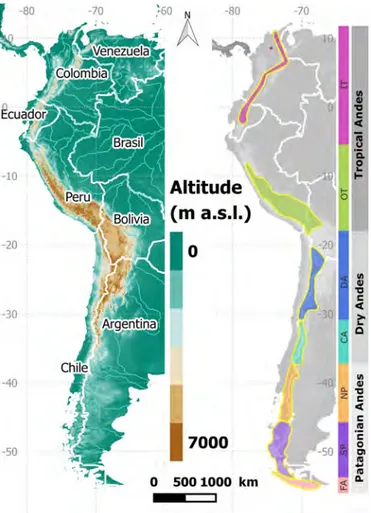
1.1.1 Geographical situation

The Andes are the longest continental mountain range of the world running across the west coast of South America over more than 7000 km from Colombia (10°N) up to the Southern-most region of Tierra del Fuego (56°S) at the Austral end of Chile and Argentina (Figure1.1). Along the tropical and subtropical portion of the Andes average elevation exceeds 4000 m a.s.l. containing the highest peak of America, the Aconcagua (32°S) at 6980 m a.s.l. and the world’s highest volcano, the Ojos del Salado (27°S) at 6890 m a.s.l. South of 35°S average heights decrease to about 1500 m a.s.l. but still containing many peaks above 3000 m a.s.l. In contrast with their longitude, the Andes stay a relatively narrow range with typical widths of 200 km and a maximum of 700 km in the subtropical region, where they split into two mountain ranges surrounding the South American Altiplano. This high elevation plateau presents average elevations of 4000 m a.s.l. and is exceeded only by the Tibetan Plateau on surface and altitude. Large rivers drain from the Andes to the Atlantic Ocean, the largest being the Amazon river with a length of 7000 km, followed by the Parana (4900 km). Towards the western slopes of the Andes, rivers reach the Pacific Ocean coasts fast, with the largest river (rio Loa) extending only 440 km.

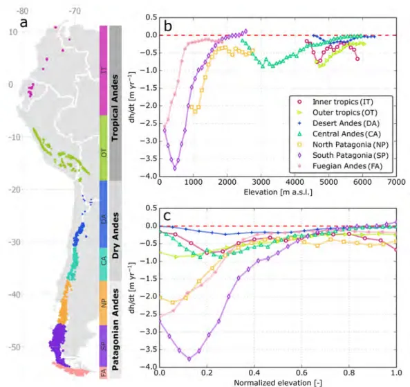
There is still no consensus on the delimitation and naming of Andean regions. As they cross along seven South American countries, generally political boundaries are referred to for simplification. For scientific aims, a wide range of possibilities have been proposed, varying greatly depending on the fo-cus of the research topic. In this manuscript I define a set of seven sub-regions according to latitude and prevailing climatic conditions and based on previous regional glaciological subdivisions (Masiokas et al., 2009; Rabatel et al., 2013a; Sagredo and Lowell, 2012). The Tropical Andes corresponds to the region North of 20°S containing the Inner and the Outer Tropics. The Dry Andes, between 17°S and 37°S encloses the Desert and Central Andes. Further South, the Patagonian Andes are divided between North Patagonia, South Patagonia which contains the two major Andean icefields: the Northern Patag-onian Icefield (NPI) and the Southern PatagPatag-onian Icefield (SPI) and finally The Fueguian Andes to the South of The Magellan Strait (Figure1.1).

(16)

1.1 Characteristics of the Andes mountain range

Figure 1.1: Elevation range of the Andes Cordillera (from SRTM 4.1 data resampled at 500 m) and the defini-tion of Glacio-climatological regions used through the manuscript.IT (Inner Tropics) and OT (Outer Tropics) correspond to the Tropical Andes; DA (Desert Andes) and CA (Central Andes) to the Dry Andes; and NP (North Patagonia), SP (South Patagonia) and FA (Fuaguian Andes) to the Patagonian Andes.

1.1.2 Climatic diversity

Consistent with its latitudinal extension and altitude, the Andes exhibit heterogeneous climate settings with Tropical, Subtropical and Extratropical features. In the Tropical (10°N-17°S) and Subtropical re-gions (17°S-37°S) large scale circulation is characterized by the Inter-Tropical Convergence Zone (ITCZ) and the Trade winds blowing from the East while westerly winds blowing from the Pacific Ocean dom-inate circulation in the Extratropical region (south of 35°S). Mean annual temperature is mostly con-trolled by latitude and elevation with a 0 isotherm that stays close to 4000 m a.s.l. at the tropical and subtropical latitudes dropping to 500 m a.s.l. at the southern tip of the continent (Garreaud, 2009;

Sagredo and Lowell,2012). The transport of moisture towards the Andes is mostly determined by the tropospheric low-level flow represented in Figure1.2(Garreaud,2009). The height and continuity of the mountain range disrupts tropospheric circulations resulting in contrasted climate conditions all along the eastern and western sides of the Cordillera (Figure1.3).

(17)

Figure 1.2: Low level tropospheric flow (below 1500 m a.s.l.) around the Andes Cordillera. The main pro-cesses responsible for moisture transport towards the Andes and the relative precipitation areas are shown. In the Tropical Andes, trade winds blow moisture from the Amazon basin and the westerly winds blow moisture from the Pacific ocean at extratropical latitudes. The Dry South American Diagonal is clearly visualized between these two major circulations. Major climate features like the South East pacific Anticyclone and cold sea surface temperatures across the Pacific coast are also shown. Figure fromGarreaud(2009)

Regional precipitation regimes

The Tropical Andes can be divided into two climatic zones, delineated by the seasonal migration of the ITCZ. The Inner Tropics (North of 5°S), present constant temperature an humidity conditions with precipitations occurring all year long. The Outer Tropics (5°S-17°S) is characterized by alternating dry season and wet seasons, with the corresponding seasonality on specific humidity, cloud cover and pre-cipitation (Rabatel et al.,2013a).

From Tropical to subtropical latitudes, wet conditions prevail along the Eastern slopes of the Andes resulting from the constant easterly flow bringing moisture from the Amazon basin (Garreaud et al.,

2003). The Tropical Andes receive most precipitations from deep convective storms that develop over the high altitude mountain range, enhancing orographic precipitation that can reach up to 6000 mm/yr at the eastern Ecuatorian Andes (Garreaud,2009;Vuille et al.,2000a,b). Contrasting arid and cold con-ditions prevail along the western slopes descending to the Pacific Ocean. This gradient reverses south of 35°S were the area of low precipitations shifts to the East of the mountain range in the Patagonian steppes of Argentina, thus creating the South American Arid Diagonal that crosses the Andes between 19-23°S (Messerli et al., 1998). The Desert Andes, located at the north of this Arid Diagonal, present mean annual precipitations decreasing from 400 mm at 18° to less than 100 mm at 23°S. The gentle de-scent of air (subsidence), enhanced by the upwelling of cold water along the Pacific coast at this latitude, maintains the subtropical anticyclone over the South East Pacific, resulting in arid and stable conditions all year long (Houston and Hartley,2003;Rutllant et al.,2003). The South American Altiplano, also in the Desert Andes, exhibits its own climate conditions. It remains extremely dry during most of the year excepting the austral summer (November-March, a period named the South American Monsoon) when intense convective storms developing in the Amazonian basin bring significant precipitations (Zhou and Lau,1998). The east-west precipitation contrast is high at this latitude, with the dry Atacama Desert in the West and the Chaco wetlands in the East, also influenced by the Monsoon summer rainstorms.

(18)

1.1 Characteristics of the Andes mountain range

Figure 1.3: Long term mean precipitation and temperature over South America. (A) Mean precipitation for Austral winter (June-July-August) and (B) summer (December-January-February). Figure from Garreaud et al 2009. (C) Mean annual temperature from the high resolution data set for surface climate model (New et al.,

2002). Figure fromSagredo and Lowell(2012).

South of 21°, precipitations are produced mostly by the passage of extratropical frontal systems ( Gar-reaud, 2009; Garreaud et al.,2009). The Central Andes are characterized by a Mediterranean climate with dry summers and cold winters. This is the result of the north to south displacement of the South East Pacific Anticyclone, inhibiting precipitation in summer and allowing the passage of westerlies and frontal precipitation in winter (Rutllant et al., 2003). Total annual precipitation ranges from 500 mm around 31°S to 2500 mm at 36°S (Pellicciotti et al.,2014). Further South in the Patagonian Andes the latitude band of maximum precipitation coincides with the location of the storm track, 45°S-55°S in summer and 35°S-45°S in winter. Precipitation maxima occur at the western slopes enhanced by mois-ture uplift by the orographic effect of the Andes. Deep rainforest and large icefields are characteristic of this wet region in the Chilean Patagonia. Extreme precipitation gradients are found here, with totals ex-ceeding 7000-8000 mm at the SPI and little moisture is left when the air masses cross toward Argentina (Lenaerts et al.,2014;Smith and Evans,2007;Villalba et al.,2003).

Inter-annual and inter-decadal climate variability

Three large scale modes are responsible for natural climate variability in South America, modulating temperature and precipitation in the Andes at interannual and interdecadal time scales (Figure1.4 Gar-reaud et al.,2009). Over Tropical and Subtropical Andes, climate variability is mostly dominated by the El Niño Southern Oscillation (ENSO) and the Pacific Decadal Oscillation (PDO) while further South is regulated by the Southern Annular Mode (SAM) (also known as the Antarctic oscillation, AAO).

ENSO is a coupled ocean-atmosphere phenomenon regulated mostly by the equatorial Pacific mean surface temperature. It is characterized by irregular fluctuations between a warm phase (El Niño) and a cold phase (La Niña) with a periodicity of 2 to 7 years (DIAZ, 1992). There is general agreement that rainfall and temperature anomalies associated to ENSO are the major source of inter-annual vari-ability over South America (Francou et al., 2004; Garreaud, 2009; Vuille et al., 2000a,b). Overall, El Niño episodes are characterized with below average precipitation over the Tropics, above average rain-fall over Subtropical South America and generalized warmer than normal air temperatures. Opposite

(19)

anomalies are observed during La Niña event, with cold and wet conditions in the Tropical region and a contrasting cold and dry Subtropical Andes. This contrasted tendencies have shown evident effects over snow pack and streamflow (e.g.Masiokas et al.,2010) and glacier mass balance (e.g.Francou et al.,

2004) in the Tropical and Dry Andes regions.

The PDO is responsible for inter-decadal changes in South American climate, characterized by a period-icity of 20 to 30 years (Mantua and Hare,2002). PDO related precipitation and temperature anomalies are similar in spatial structure to ENSO (i.e. they present an ENSO Like pattern) but their effect is less intense (Garreaud et al.,2009). Previous studies have shown El Niño (La Niña) rainfall anomalies to

be stronger during the warm (cold) phases of PDO (Andreoli and Kayano, 2005). The PDO effect on

glaciers is also similar to that of ENSO. A climatic shift from a cold to a warm PDO phase has been observed after 1976/77 where El Niño events have become more frequent and intense compared to previous decades, with clear impacts on natural systems and water resources (Garreaud et al., 2009;

Mantua and Hare,2002).

The SAM is the leading pattern of interannual variability over the southern tip of South America ( Gar-reaud et al.,2009;Gillett et al.,2006). It is characterized by pressure anomalies of one sign centered on

the Antarctic and anomalies of opposite sign on a circumpolar band at about 40°-50°S (Thompson and

Wallace,2000). The positive phase of SAM is associated with a strengthening and poleward shift of the westerlies, enhancing dry conditions and warm air temperatures across Patagonia and contrasted cold-wet conditions in Antarctica. The SAM has shown a marked trend towards its positive phase during the

last decades, increasing the temperatures in southern South America (Thompson and Solomon,2002;

Villalba et al.,2012). However, the effect of SAM over Andes glaciers is still poorly known.

Figure 1.4: Annual mean precipitation and surface air temperature fields regressed upon ENSO Index, PDO Index and SAM or AAO Index.The value of the regression coefficient β indicates the local anomalies in the field (in physical units: mm or °C) associated with a unit anomaly of the index. This figure helps visualizing the similar spatial structure of the ENSO-related and PDO-related and anomalies, the reduced amplitude of PDO compared with ENSO, and the influence of SAM over the Southernmost latitudes. Figure fromGarreaud et al.(2009)

(20)

1.2 Andes Glaciers

1.2.1 Glacier inventories

The wide variety of topographic and climatic conditions described above, result in a large diversity of ice masses along the Andes Cordillera. The magnitude and spatio-temporal distribution of precipita-tion and temperatures will determine the possibility of glaciers to exist in some locaprecipita-tions and not others. Before studying glaciers, we need to know where they are located and how large they are, this is repre-sented in glacier inventories. The interest on knowing where Andean glaciers are is quite recent com-pared to the rich glaciological legacy existing for example, in the European Alps. The first photographs and historical maps of glaciers were produced by the first explorers of the Andes at the beginning of the 20th century (e.g. Dr. Federico Reichert, Padre Alberto de Agostini) and the first known inventory of Andes glaciers was published only in 1956 by Louis Lliboutry, the French researcher, pioneer in South American glaciology, and was restricted to glaciers located in the Chilean Andes (Lliboutry,1956). In recent decades, with the birth and development of satellite remote sensing techniques, more pre-cise and standardized glacier outlines have been produced from optical satellite images, permitting to map glaciers at a global scale with high precision. Semi-automatic methods based on the differential reflectance of snow and ice on the visible and the shortwave infrared bands permit to distinguish ice and snow from other surfaces (Paul et al.,2015). However, this methodology is far from being exact and posterior manual editions are usually recommended by the Global Land and Ice Measurements from Space (GLIMS) initiative (Racoviteanu et al., 2009). In general, errors due to the interpretation of glacierized surfaces from satellite scenes are around 5% for exposed ice and up to 30% for debris covered glaciers (Paul et al.,2013).

Geographical institutions in most South American Andean countries have produced independent, high quality and multi-temporal glacier inventories for all glaciers within their territories. However, com-bining these revised inventories to obtain an inventory at the entire Andes scale is not straightforward: (i) there is no methodological homogeneity in the way these inventories were created. (ii) They are tem-porally heterogeneous, representing glacier extents for a wide range of dates. (iii) The data is not always freely accessible. To my knowledge only Peru (www.ana.gob.pe), Argentina (www.glaciaresargentinos.gob.ar) and Chile (www.dga.cl) allow free access to complete glacier inventories. And finally, (iv) political is-sues between countries have induced unrealistic glacier outline interpretations. For example, glaciers at the border between Chile and Argentina are defined with the political limits rather than the real glacio-logical limits, and there are still conflict zones involving glaciers like in the SPI, where the limit zone is not demarcated and mapping is restricted (e.g. Chilean-Argentinian Treaty, 1998). This denotes the strong need for South American countries to joins efforts in the homogenization of glacier inventories, where politics need to be set aside in the favour of science.

Until now, the only complete and homogeneous glacier inventory covering the entire Andes range is the Randolph Glacier Inventory (RGI, Pfeffer et al., 2014). RGI, currently on its 6th version, is a global inventory of glacier outlines covering all 19 glacierized regions of the world, supplemental to the GLIMS dataset and intended to support glacier research and monitoring worldwide. The Andes are contained within two regions, RGI region 16, corresponding to Low Latitudes, where more than 99% of the glacierized area of this region is concentrated in the Tropical Andes; and RGI region 17, corresponding to the Southern Andes. Outlines represent ice extents of years from 2000 to 2003. Its quality is good enough for regional studies and it has been widely used before for Andes-wide glacier change estimations (Braun et al.,2019) and for glaciological and hydrological modelling (e.g.Huss and Hock,2018;Marzeion et al.,2015). Large Icefields and some individual glaciers have been updated with high quality independent outlines; however, there is no doubt that many zones could still be improved, especially small mountain glaciers and snow patches are incorrectly mapped in the current RGI v6.0.

(21)

1.2.2 Spatial distribution of Andes glaciers and their characteristics

The RGI glacier inventory gives insight in the spatial distribution of Andean glaciers, which is strongly linked with altitude and the varying climate contexts. Glaciers cover a wide range of altitudes from the highest peaks and volcanoes above 5000 m a.s.l. in the Tropical and Subtropical Andes to sea level in Patagonia and Tierra del Fuego (Figure1.5). From the Desert Andes to the South, the glaciers mean altitude starts descending progressively until altitudes bellow the 500 m a.s.l. at the southern edge of the continent. Largest glaciers are found at the lowest altitudes in the Patagonian Andes, more particularly in the large NPI, SPI and Cordillera de Darwin Icefields (Figure1.5).

Figure 1.5: Latitudinal and regional distribution of Andean glaciers as a function of the mean altitude.Glacier surface area is depicted with the size of the circles.

1.2.3 Sensitivity to climate and seasonal cycle

Regional climates play an important role in modulating glacier response to climate variability (Fujita,

2008;Oerlemans and Reichert,2000;Rupper and Roe,2008;Sagredo et al.,2014). Understanding the sensitivity of a glacier is key for the interpretation of past, present and future glacier fluctuations. In the Andes, the wide variety of climatic conditions result in a large quantity and diversity of ice masses (Clapperton, 1983; Garreaud et al., 2009; Sagredo and Lowell, 2012), resulting in important variability in glacier sensitivities, particularly to air temperature, to the total amount of precipitation received and to its seasonality. Glacier sensitivity is usually defined as the change in mass balance in-duced by a 1°C change in temperature or a 10% change in precipitation. In general, the sensitivity to temperature and precipitation changes increase dramatically with the amount of annual precipita-tion (Cogley et al.,2011). For this reason, glaciers located in maritime climates (Patagonian Andes) or tropical climates (Tropical Andes) presenting high rates of mass turnover, are usually more sensitive to climate changes (Meier,1984;Oerlemans and Reichert,2000).

Glaciers receiving precipitation during the summer months (i.e. summer accumulation type glaciers) are more sensitive to warming than those receiving precipitation only during the winter months (i.e. winter accumulation type glaciers). For summer accumulation type glaciers warming (i) prolongs the

(22)

1.2 Andes Glaciers

duration of the melting period, (ii) causes a significant decrease in summer snow accumulation, because precipitations fall as rain in a warmer environment, and additionally (iii) decreases the glacier surface albedo enhancing the absorption of solar radiation and therefore melt (Fujita,2008). In opposition, for winter accumulation type glaciers, warming only prolongs the melting period without changing snow-fall in summer. Sensitivity of these glaciers is mostly controlled by the duration of the ablation season and the differences between melting and sublimation rates (Kaser,2001).

Tropical (Low Latitude) glaciers are amongst the most sensitive glaciers of the world (Kaser, 2001). The great majority of low latitude glaciers are located in the Andes mountains. In the Inner Tropics, glaciers are summer type: the continuous humid conditions and stable temperatures causes accumula-tion and ablaaccumula-tion to occur simultaneously all year, during summer and winter (Figure 1.6,Kaser and Georges,1999;Rabatel et al.,2013a). Interannual mass balance variability is mainly controlled by the air temperature, which determines the snowline altitude, as observed in the vertical mass balance pro-files for this region (Figure1.6, Kaser and Georges, 1999; Francou et al., 2004; Kaser,2001). Glaciers in the inner tropics are highly sensitive to warming, but seasonal snowfall also plays an important role controlling the surface albedo that will determine the intensity and duration of the melt season, partic-ularly during the period when solar radiation is strong (Rabatel et al.,2013a).

Glaciers in the Outer Tropics are winter accumulation type glaciers: the tropical conditions in winter causes ablation and accumulation to occur simultaneously, but in summer the dry subtropical

condi-tions makes accumulation almost inexistent and most of the ablation occurs by sublimation (Wagnon

et al.,1999) (Figure1.6). These glaciers are mainly sensitive to the seasonal distribution of precipitation but also to the total amount (Favier et al.,2004;Francou et al.,2003;Wagnon et al.,2001). Inter-annual mass balance variability depends mostly on the beginning of the wet season, with any delay causing very negative mass balances due to reduced snow accumulation, low albedo and large ablation rates (e.g. during El Niño events,Rabatel et al.,2013a;Wagnon et al.,2001).

(23)

Figure 1.6: Schematic comparison of Inner Tropical, Subtropical and Extratropical-Midlatitude glacier mass balance regimes and their corresponding modelled vertical mass balance profiles. Note that at the x-axis changes in mass balance are in respect to the mass balance at the 0°C level. Figure modified fromKaser and Georges(1999)

In the extremely dry Desert Andes (Subtropics) glacier accumulation is sparse, coming from oc-casional precipitations, and almost all ablation result from sublimation (Ginot et al.,2006;MacDonell et al.,2013;Gascoin et al.,2013). Most of these high altitude glaciers are located above the 0°C isotherm and are rarely exposed to melting temperatures (Sagredo and Lowell,2012). They are strongly sensitive to changes in air humidity, which controls the amount of precipitation but more importantly, affects the balance between melt and sublimation (Kaser,2001;Rabatel et al.,2011).

In Southern regions at midlatitudes (Central Andes to Patagonia), accumulation occurs during win-ter and ablation during summer (Figure1.6), with the exception of maritime glaciers located close to the South Pacific coast in Patagonia and Tierra del Fuego, which receive precipitations all year long. Sublimation is still important in the Central Andes but becomes almost negligible in the Southern-most regions where melt dominates. Continental glaciers in this regions, are sensitive to the amount of precipitations, while the effect of temperature is only significant during summer months, because it favours melt and increases the duration of the ablation season (Oerlemans and Reichert, 2000). Mar-itime glaciers are more sensitive to temperature changes, and their mean annual temperature is strongly dependent on the sea surface temperature (Kerr and Sugden,1994). Warming in maritime glaciers in-duces high melt rates at the glacier tongue and increases the altitude of the 0°C isotherm, reducing significantly the fraction of precipitation falling as snow (Oerlemans and Reichert,2000).

The glacier equilibrium line altitude (ELA), is also used as a proxy for sensitivity of glaciers to their climate. The ELA is the altitude at which the glacier surface mass balance is equal to 0, with accumu-lation occurring above and abaccumu-lation below. It can be approximated by the annual maximum altitude of the snowline (Rabatel et al.,2005). The ELA is also sensitive to climate conditions, and directly affects

(24)

1.2 Andes Glaciers

ELA changes are strongly tied to the dominant ablation process. In regions where melt is dominant, the ELA is more sensitive to air temperature, while in sublimation dominant regions, the ELA is more sen-sitive to precipitation (Rupper and Roe,2008). In the Andes, the ELA sensitivity to temperature reveals variations between 140 to 230 m for every 1°C in temperature change, with the Inner Tropics being the most sensitive region (larger melt rates) and the Desert Andes the less sensitive (larger sublimation rates)(Sagredo et al.,2014). Similarly, the ELA was shown to be more sensitive to precipitation in the Desert Andes (dry climate), than over regions like the Inner Tropics and Patagonia, presenting humid climates and frequent cloud cover (Sagredo et al.,2014).

Hydrological context and contribution to streamflow

The seasonal fluctuations of glaciers are very important for hydrology as they can significantly modify the quantity and timing of streamflow even in catchments where the ice cover is relatively low (Radić

and Hock,2014). There are still considerable ambiguities with respect to the definition of glacier runoff,

and therefore, no consensus on the way to quantify it. The runoff originating at the glacier terminus has different origins, it may come from the melt of ice, snow or firn, but it may also come from rain on the glacier or melting from the snow located outside the glacier, and is also affected by processes like evaporation, sublimation and refreezing of liquid water. Different concepts generally used in literature vary essentially on those that include or not the snow accumulation and the water coming from the glacier that has not been generated from melt (Radić and Hock,2014).

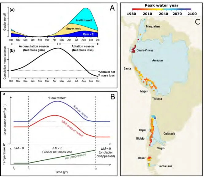
Glacier runoff can be considered as a function of annual or multiannual glacier volume changes, and can be directly linked to glacier-wide mass balance measurements (see section1.3). In this case, glaciers runoff is considered as an ‘excess discharge’ of water originating from the glacier volume changes during a particular period (Lambrecht and Mayer,2009;Pritchard,2019), and directly represents the imbal-anced condition of the glacier. This concept assumes that glaciers produce runoff only when they are losing mass (they are imbalanced), and their contribution is zero when they are in balance or present positive volume changes. Thus, this so-called imbalanced glacier contribution to runoff stands as a di-rect measure of the perennial changes in glacier water storage and represents an important measure of the sustainability of glaciers as future water resources. In this thesis work, I will estimate the decadal imbalance glacier contribution of glaciers over seven important Andean river basins during the last two decades, and how the interdecadal variability of glacier contribution is linked with climate. This volumetric approach, however, is not very useful for hydrologists because in fact glaciers influence streamflow on a seasonal scale, even when they are in balance with their climates (Huss, 2011; Kaser et al.,2010;Radić and Hock,2014). In winter accumulation regimes, when the accumulation period is different form the ablation period, there is a delay between the moment (winter) when water is stored

on the glacier, and the moment (summer) when melt water is produced (Figure1.7A). This is called

the seasonally delayed runoff and plays an important role sustaining river flows during the dry season or during periods of extreme drought, compensating for otherwise reduced flows, specially when rivers are located in arid and semiarid regions (Huss and Hock,2018;Kaser et al.,2010;Radić and Hock,2014).

(25)

Figure 1.7: Panel A:(a) Schematic seasonal variation of total runoff and its components, E is evaporation. (b) Cumulative glacier mass balance in specific units (m w.e. yr-1) showing a year with negative mass balance. Figure fromRadić and Hock(2014). Panel B: Schematic illustration of the changes in runoff from glacierized basin in

response to continuous atmospheric warming. Figure fromHuss and Hock (2018). Panel C: Peak water in all the glacierized macroscale drainage basins. Figure fromSchoolmeester et al.(2018), data fromHuss and Hock

(2018).

Several studies have attempted to document the glacio-hydrology in the Andes, with a concentrated attention on the most vulnerable zones, the Tropical Andes and some selected catchments at the arid and semiarid regions of Chile and Argentina. In a global scale study,Kaser et al.(2010) used a monthly glacier melt model comparing glacial melt inputs with precipitation patterns to assess the effect of glaciers on seasonal water resources in glacierized basins around the world. For the Andes, they studied only the Santa river basin in Peru, where climate is arid and maximum ablation rates are synchronized with the dry season. Seasonally delayed glacier contribution in the Santa basin showed to reach a max-imum (January) of 71% of the total runoff at the glacier front (Kaser et al.,2010). Similar contributions were found by other modelling approaches, showing that almost 38% of the Santa total annual flow comes from melting glaciers (Buytaert et al.,2017;Condom et al., 2012;Vergara et al.,2007). Similar results where also found in Bolivia (Soruco et al.,2015). Buytaert et al.(2017) coupled the model from

Kaser et al.(2010) with a regional water balance model of the Tropical Andes and high resolution spa-tial data on water use along the watershed. They found a large seasonal variation in the contribution of glacial melt and persistent strong glacier contributions on all arid and semiarid Pacific basins and on those located in the Altiplano of South Peru and Bolivia. Glacier contribution to streamflow is max-imum at glacier front and decreases downstream, consequently the glacier contributions calculated in the above mentioned studies are valid only for a specific location in the basin.

(26)

1.2 Andes Glaciers

In the Desert and Central Andes of Chile, glacier contribution to river discharge is also considerable, reaching maximum values of 50% and 58% of the total runoff at the outlet of Glaciar Bello and Uni-versidad during enhanced periods of drought (Ayala et al., 2016; Bravo et al., 2017), and up to 47% at the outlet of Juncal Norte in the late ablation season (Ragettli and Pellicciotti,2012). Mean annual glacier contributions can reach up to 23% in basins with less than 11% glacier coverage (Gascoin et al.,

2011). This estimates are however, not free of uncertainties, most of them regarding the non consider-ation of the sublimconsider-ation fluxes, known to be important in the arid and semiarid regions (e.g.Wagnon et al.,2001), groundwater contribution to streamflow during the dry season, which has been suggested to be considerable in semiarid basins (e.g.Rodriguez et al.,2016). In many cases the lack of reliable and continuous streamflow data and regional glacier change assessments in this vulnerable regions do not allow to perform regional estimates of glacier contribution to streamflow.

Concerning the future of glacier meltwater availability in the Andes, in an assessment of the hydro-logical consequences of glacier decline around the world, Huss and Hock (2018) project the largest summer month reductions in glacier runoff over Central Asia and the Andes for the end of the century. Noticeably, they are also the two regions of the world where more than 50% of the total basin runoff comes from snow and ice (Huss et al.,2017). Glacier in the Andes have experienced continuous retreat during the last decades (Casassa et al., 2007; Pellicciotti et al., 2014; Rabatel et al., 2013a). When a glacier is in balance with its climate, its annual contribution to streamflow stays constant through time, but when a glacier is exposed to a warming climate, it retreats and water is released from its long-term storage (i.e. glacier imbalance contribution). As a consequence, glacier runoff is expected to increase until reaching a maximum ‘peak water’ beyond which runoff starts to gradually decrease, because the reduced glacier volume cannot support high melt rates anymore (Figure1.7B, Huss and Hock, 2018). If temperatures continue to increase, the glacier will end up disappearing. If the glacier reaches a new equilibrium with a decreased volume, the water released during the melt season is expected to decrease bellow the initial value when the glacier was larger (as expressed by the red line in figure 1.7). Most of the Andes basins dominated by small glaciers have already reached the peak water or it is expected to occur within the next decades (Figure1.7C,Gascoin et al.,2011;Bravo et al.,2017;Huss and Hock,

2018;Vuille et al.,2018).

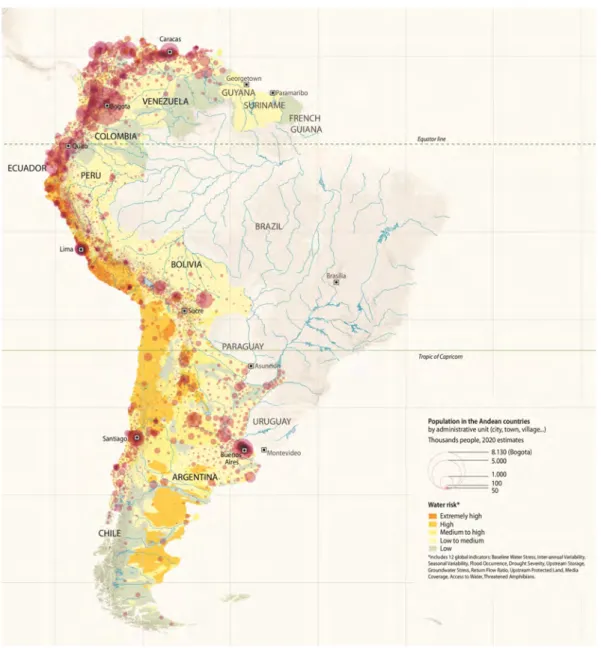
Because they hold large populations that are dependent on meltwater during summer, the Tropical and the Dry Andes regions are the most threatened by the projected glacier changes, specially during enhanced periods of droughts. The intense negative effects of an uncommonly long period of drought in the Central Andes have already been documented. This so called “mega-drought” has also been readily observed in terms of decreased streamflow, rainfall, snow accumulation and vegetation productivity, among other indicators (Garreaud et al.,2017;Rivera et al.,2017). The influence of this mega-drought on glacier changes in the Dry Andes is an important aspect that will be considered in this work. The high impacts on water resources are expected to affect socioeconomic activities such as agriculture and hy-dropower, which are in many cases the principal economic activities of many Andean countries (Bradley et al., 2006; Buytaert et al.,2017; Vuille et al.,2018). The United Nations Educational, Scientific and Cultural Organization (UNESCO) recently evaluated water risk in the Andes considering different in-dicators and the population growth expected for 2020 (Figure 1.8, Schoolmeester et al., 2018), it is interesting to see that the regions with high risk coincide with the regions where glacier melt help sustain streamflow during the dry seasons. This stresses the need to constrain glacier changes in this regions and start thinking about mitigation policies.

(27)

Figure 1.8: Population and water risk in Andean countries. Population estimates for 2020 by administrative unit (city, town). Water risk includes 12 global indicators: Baseline water stress, Inter-annual variability, Seasonal variability, Flood occurrence, Drought severity, Upstream storage, Groundwater stress, Return flow ratio, Up-stream protected land, Media coverage, Access to water and Threatened amphibians. Figure fromSchoolmeester et al.(2018)

1.3 What is the glacier mass balance?

1.3.1 Glacier mass balance as an indicator of glacier health

Glacier are recognized as sensitive indicators of climate changes (Oerlemans, 2001). Glacier surface area and length fluctuations have been used historically as observations of glacier evolution in the An-des (e.g.Aniya et al.,1997;Aniya and Enomoto,1986). However, these variables are indirect climatic indicators as they result from a combination of both climatic forcing and glacier dynamics, which is unique to every glacier and is determined by its slope, exposition, the state of the glacier surface (ice or debris covered) and the type of glacier front (if its terminates on land, a lake or the ocean).

Glacier mass balance is a measure of the evolution of the quantity of snow and ice that is stored in the glacier, directly linked to variations in accumulation (precipitation) and ablation cycles (temperature and energy fluxes) (Cuffey and Paterson,2010). Mass balance annual series and the spatial distribution of these changes with altitude allow to detect changes in climate (Oerlemans,2001). In this sense, an unhealthy glacier is not in equilibrium with its climate, presenting sustained (year to year) negative mass changes that can ultimately lead to its disappearance.

(28)

1.3 What is the glacier mass balance?

In simple terms, the mass balance ( ˙b) at a specific point of a glacier is defined as the difference between the accumulation and the ablation (Cuffey and Paterson,2010).

˙b = accumulation − ablation (1.1)

Where mass gains may come from multiple sources such as snowfall, avalanches, wind snow distribu-tion or refreezing of the liquid water infiltrating the glacier. Abladistribu-tion is governed by different processes including melt of snow and ice, sublimation of snow and ice and losses due to the rupture of icebergs or seracs at the glacier front, depending if the glacier ends in a water body or not.

The glacier-wide surface mass balance ( ˙B) is obtained by integrating the specific mass balance ( ˙b) on

the entire glacier area (A) (Cuffey and Paterson,2010):

˙ B = 1 A Z A ˙bdA (1.2)

Note that glacier-wide surface mass balance ( ˙B) is not equal to the total glacier-wide mass balance (4M).

Most direct observations neglect internal and subglacial mass balance changes, usually accepted to be an order of magnitude less than surface fluxes. Glacier-wide surface mass balance estimate ( ˙B), also omits

frontal ablation, that corresponds to the sum of the mass loss by calving, subaerial frontal melting

and sublimation above the water line, and subaqueous frontal melting below the water line (Cogley

et al.,2011). Mass losses by frontal ablation (specially calving) can be significant and even dominant on glaciers that end on water bodies (Sakakibara and Sugiyama,2014;Truffer and Motyka,2016) like many glaciers in the Patagonian Andes that finish in lakes or the ocean (Warren and Aniya,1999). Over these glaciers, the glacier-wide mass balance (4M) need to account for frontal ablation (Af) and is expressed

as:

4_{M = ˙}_{B + A}_f _(1.3)

Or it can be simplified as a function of calving (D) when subaerial frontal melting, sublimation and subaqueous frontal melting are negligible.

4_{M = ˙}_{B + D} _(1.4)

As a convention, mass balance is measured at the end of the ablation season of the hydrological year (end of spring, generally March-April in the Southern Hemisphere (Masiokas et al.,2016;Rabatel et al.,

2013a). It is generally expressed as a surface unit in the form of meter water equivalent per year (m w.e. yr−1). Figure1.9represents the evolution of the specific mass balance through the hydrological year for the different areas of a glacier (Cuffey and Paterson,2010). The accumulation zone is characterized by a positive mass balance, conversely in the ablation zone the mass balance is negative. These two zones are divided by a line where the annual mass balance is equal to zero (i.e. accumulation equals ablation), also defined as the equilibrium line. The ELA may vary from year to year determining the accumulation area ratio (AAR), or the ratio between the accumulation areas and ablation areas of the glacier .