ATTEL PERFORMANCE-BASED APPROACHES FOR HIGH STRENGTH TUBULAR COLUMNS AND CONNECTIONS UNDER EARTHQUAKE AND FIRE LOADINGS - D6

ATTEL

PERFORMANCE-BASED

APPROACHES FOR HIGH

STRENGTH TUBULAR COLUMNS

AND CONNECTIONS UNDER

EARTHQUAKE AND FIRE

LOADINGS

Deliverable 6:

“Design Guidelines and proposal

for EC3, EC4 and EC8”

Contributors:

University of Thessaly

University of Liège

Centro Sviluppo Materiali

Stahlbau Pichler

University of Trento

D.6

2

Table of Contents

1. Structural solution ... 3

1.1 Building structures in low-seismicity areas ... 3

1.1.1 Columns ... 3

1.1.2. Slabs and joints ... 4

1.2 Building structures in areas of significant seismicity ... 4

1.2.1 Columns ... 4

1.2.2. Beam- to- column and column-base joints ... 4

2. Global analysis of frames ... 5

2.1 Building structures in areas of low seismicity ... 5

2.2 Building structures in areas of significant seismicity ... 5

3. Design of high-strength steel CHS columns ... 5

3.1 Design of high-strength steel CHS columns at normal temperature ... 5

3.1.1 Cross-sectional strength for axial loading ... 6

3.1.2 Cross-sectional strength for bending loading ... 6

3.1.3 Strength of CHS columns ... 7

3.2 Design of high-strength steel CHS columns at elevated temperature ... 8

4. Design of column base subjected to combined bending moment and axial force ... 8

4.1. Static column-bases under static loading ... 8

4.1.1. Introduction ... 8

4.1.2. Tube and tube-to-plate weld ... 9

4.1.3. Plate in bending, bolts in tension and concrete in compression ... 9

4.2. In elevated temperature conditions (fire) ... 11

4.3. Additional guidelines on the design of seismic column-base joints ... 11

4.3.1 Standard seismic column-base joints ... 11

4.3.2 Innovative seismic column-base joints ... 11

4.4. Guidelines on the design of seismic column bases made of HSS subjected to fire loading... 12

5. Design of beam-to-column joints ... 12

5.1. Static beam-to-column joints ... 12

5.1.1. General ... 12

5.1.2. Longitudinal slap reinforcement in tension, bolts in shear and plate in bearing ... 13

5.1.3. Through plate and column in diagonal compression ... 13

5.1.4. In elevated temperature conditions (fire) ... 14

5.2. Additional guidelines on the design of seismic beam-to-column joints ... 14

Appendix A: static column base ... 16

Appendix B: Through plate of static joint ... 28

Appendix C: Cross-Sectional Strength of high-strength steel tubular members ... 34

3 This document constitutes the final deliverable from European RFCS project ATTEL. Design guidelines and optimization of the design of structural configurations such as base joints, HSS columns and composite beam-to-column joints are proposed taking into account the experimental and numerical results obtained within the project.

Design guidelines for steel buildings with high-strength steel CHS

columns

In this design guidelines for buildings for which high-strength steel can give an economical solution are presented; the reference buildings 1 and 2 (see WP2) in the present project are examples of buildings for areas of low and high seismicity respectively. For these building, static, seismic and fire actions are considered; design guidelines from global structural analysis to the verification of structural elements (e.g. column bases, tubular columns and beam-to-column joints) are proposed.

It should be noted that the present guidelines (a) are in-line with the current EN 1993 design practice and (b) propose some possible amendments for high-strength steel(HSS) tubular CHS members. The proposed amendments are based on the imperfection and residual stress measurements, the test data and the numerical results obtained within the present research project, for the seamless CHS tubes described in the previous sections of this report. A list of publications is offered, which support the proposed guidelines.

1. Structural solution

1.1 Building structures in low-seismicity areas

A cost-efficiency study has been carried out within the present project [11]; from the latter, the following conclusions can be drawn for the definition of a structural solution where HSS can have an economical interest.

1.1.1 Columns

(1) For isolated steel columns: stocky columns are recommended and the interest of using HSS decreases when the eccentricity of the axial load increases.

(2) For columns in frames: a global schematic view on the interest of using high-strength steel in comparison with normal steel (NS)/S355 is presented in Table 1. Possibilities for using high-strength steel are quite large when considering braced/non-sway frames using steel columns. On the other hand, there is no benefit in using high-strength steel for steel columns in sway frames, if compared to frames using normal steel. Moreover, for frames using composite columns, very few possibilities for using HSS can be identified.

Table1. Summary of the conclusions of the analysis

(3) In fire condition: almost no economic interest exists in using columns made of high-strength steel without protection, in both steel and composite columns. If a protection is used, the use of high-strength steel may lead to benefits as it is the case for normal temperature.

4 Accordingly, in the next section, mainly guidelines for braced/non-sway frames will be recommended/derived.

1.1.2. Slabs and joints

The following solutions for slabs and joints are suggested for a braced/non-sway frame using high-strength steel tubes for the columns.

(1) Using composite floors with a concrete/composite slab connected to the steel beams through shear connectors in order to activate a composite action at the joint level

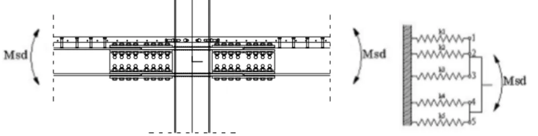
(2) Using configurations for column bases and beam-to-column joints as shown in Fig.1. The column bases are formed by one full end plate welded to the column and anchored in the concrete block by four anchor bolts. With respect to the beam-to-column joint configuration: one through plate is welded to the column, on this plate two horizontal plates (each side of the column) are attached by fillet welds. The lower flanges of steel beam are connected to the horizontal plates using bolts.

Fig.1. Suggested beam-to-column joint and column base for frames subjected to static loads 1.2 Building structures in areas of significant seismicity

Building structures subjected to medium-high seismic loadings are usually realized using moment resisting frames only along one direction. This is customarily done to contain the cost of joints designed satisfying capacity design rules. A cost-efficiency study was carried out considering the 2D moment resisting frame, see Fig.2, of the prototype structure. In detail both the design and the economic evaluation of the frame were realized considering four different solutions of circular columns: i) hollow columns with mild steel, NS S355; ii) composite columns with mild steel, NS S355; iii) hollow columns with high strength steel, HSS S590; iv) composite columns with high strength steel, HSS S590.

1.2.1 Columns

The analysis conducted on the different solutions showed the advantage of using high-strength steel S590 with respect to the mild steel NS S355. In fact the use of columns endowed with high-strength steel with the same geometry of the columns realized with mild steel complies with capacity design rules. This does not require the increase of the column sections with economic savings of about 15%.

1.2.2. Beam- to- column and column-base joints

The solutions suggested for beam-to-column and base-column joints with columns with HSS follow: (1) beam-to column joints designed as rigid and full strength joints and realized by bolted connection, as showed in Fig. 1. A vertical through plate and two horizontal plates were welded to the column in order to bolt the beams by means of cover plates. The use of composite columns exhibits better strength and stiffness than simple connections to the tube face. In fact, this connection avoids all possible phenomena of large instability in the wall around the joint region.

5 (2) Two solutions for column-base joints: i) a standard solution with base plate, anchor bolts and vertical stiffeners; ii) an innovative solution with a column embedded in the concrete foundation. Both the plate welded around the column and the four anchor bolts are used for column erection purposes.

Beam-to-column joint Standard base Joint Innovative base-joint

Fig.2. Suggested beam-to-column joint and column bases, standard and innovative, for MRF subjected to seismic loads

2. Global analysis of frames

2.1 Building structures in areas of low seismicity

(1) During the construction phase: the behaviour of beam-to-column joints as illustrated in Fig. 1 must be considered as hinges. The column base behaviour may be considered as semi-rigid and partial strength. Globally, elastic analysis for simple steel frames should be adopted.

(2) During the exploitation phase: both beam-to-column joints and column base can be considered as semi-rigid and partial strength joints. Globally, elastic/plastic analyses for semi-continuous composite frames could be applied.

2.2 Building structures in areas of significant seismicity

The behaviour of both beam-to-column and column-base joints, showed in Fig 2, could be assumed as rigid and full strength both during the erection and exploitation phases. In particular, the configuration of column-base joints is the same in both phases; even though beam-to column joints lack the presence of the composite action during erection, they are rigid and full strength anyway. In this phase, in fact, the strength is assured by the slip resistance owing to preloaded bolts used in connections. Both the joints and the structures can be assumed to belong to a medium ductility class during structural analysis under seismic loading. These properties were confirmed by test results.

3. Design of high-strength steel CHS columns

3.1 Design of high-strength steel CHS columns at normal temperature

The design procedure follows the general framework of EN 1993 parts 1-1 [2] and 1-6 [3]. The rules in EN1993-1-1 (Sections 6.3.1-6.3.3) can be used, following the existing classification (see Appendix C),

6 shown in Table 2. This design procedure results in safe, yet conservative predictions. However, some amendments to these rules are proposed, to account for the above conservativeness for high-strength steel CHS seamless members, similar to the tubes considered in the present work [4] [5], with wrinkling imperfection amplitudes not exceeding 2.6% of the tube thickness (see Appendix C).

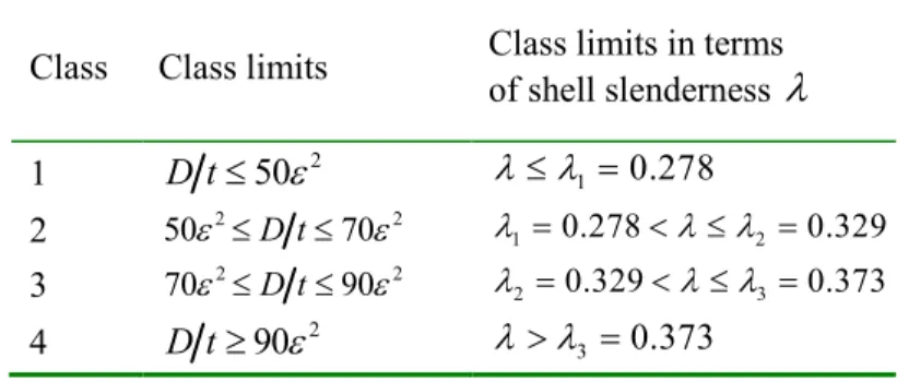
Table 2. CHS member classification according to EN 1993-1-1

Class Class limits Class limits in terms of shell slenderness

λ

1 2 50 D t≤ ε λ ≤λ1 =0.278 2 2 2 50ε ≤D t≤70ε λ₁ =0.278<λ ≤λ₂ =0.329 3 _70ε2_{≤D t≤90ε}2 2 0.329 3 0.373 λ = <λ ≤λ = 4 D t≥90ε 2 λ >λ3 =0.373

3.1.1 Cross-sectional strength for axial loading

Shell slenderness is defined as follows [3]: y

e

σ

λ=

σ

(1)

where σy is the yield stress and

e x

t σ =0.605C E

r (2)

For member slenderness λ ≤0.60, the axial compression load is calculated as follows:

NRk=σyA if λ ≤λ =0.3733 (3) 3 3

-Rk y

N

A 1-

_α α

λ λ

σ

β

λ λ





=

_

_





if

λ λ

> 3 (4) where βa=0.133,

λ

_α=0.6 and

λ

₃=0.373.

The above equations are valid for values of shell slenderness

λ

less than 0.60, and are shown in Fig.3b, together with test data and numerical results [4].

3.1.2 Cross-sectional strength for bending loading

The value of shell slenderness λ is obtained from the equation (1). The bending strength of the cross section is calculated as follows:

MRk=Mp=σyWpl if λ ≤λ =0.329₂ (5) 2 2

-

1

-Rk p b b

M

M

β

λ λ

λ λ





=

_

_





if

λ λ

> 2 (6) where βb=0.22,

λ

b=0.5and

λ

2=0.329

The above equations are valid for values of shell slenderness

λ

less than 0.60, and are shown in Fig.3a, together with test data and numerical results [4].

7

Fig.3a Bending capacity versus shell slenderness [4].

Fig.3b Axial load capacity versus shell slenderness [4].

3.1.3 Strength of CHS columns

The strength of tubular members under combined loading of axial load and bending is calculated from the interaction curve proposed by EN-1993-1-1 paragraph 6.3 [2]:

Ed Ed

Rk Rk

N M

+k =1

χN M (7)

where MEd and NEd are the acting axial and bending loads, and NRk, MRk represent the cross sectional axial and bending strength respectively (defined above). The k factor is a coefficient that depends on axial load and the shape of the bending moment diagram along the members, defined in Annex A or B of EN1993-1-1. The buckling reduction factor χ depends on column slenderness

8 Rk e

N

λ=

N

(8)

where Ne is the elastic buckling load of the tubular column. Note that the above definition of λ accounts for CHS sections which may not reach the full plastic axial load. Finally, it is recommended to use curve α0, for the reduction factor χ(λ) as defined in EN1993-1-1 [2]. More FE results are reported in Appendix D.

3.2 Design of high-strength steel CHS columns at elevated temperature

The following remarks should be kept in mind for the design of these columns in fire conditions (elevated temperature).

(1) The design of circular columns made of HSS under fire action should be based on Eurocodes 3, part 1-2 [6], and Eurocode 4, part 1-2 [8] for steel and composite columns respectively.

(2) The use of stress-strain relationship at elevated temperature initially developed for carbon steel provided results that well reproduced the prediction of vertical displacements, if compared to the experimental results. Also, for the circular filled tube column, the fire resistance predicted with the Eurocode rules was in good agreement with that found experimentally.

(3) However, the fire resistance of the tested steel columns was overestimated using the material model of Eurocode 3, part 1-2 [6]; the so-obtained predictions are significantly influenced by the considered initial imperfection. To obtain a fire resistance in line with the experimental evidence, the imperfection shall not be taken less than L/200, which is not in line with the recommended initial imperfection for such elements. This aspect should be investigated in more details, what constitutes a perspective to the present project.

4. Design of column base subjected to combined bending moment and axial force

4.1. Static column-bases under static loading 4.1.1. Introduction

(1) Three parts should be considered at the level of the column base: • column (steel tube);

• tube-to-plate weld;

• end plate in bending, anchor bolts in tension and concrete in compression.

(2) The bending moment-axial resistance interaction zone for the whole column base is defined from the ones of the joint components (Fig.4). The way to characterise these components is given here below.

9

4.1.2. Tube and tube-to-plate weld

Resistance of the components “tube” and “tube-to-plate weld” can be calculated using Eurocode 3, part 1.1 [2]. The bending moment-axial resistance interaction curves for these components can be easily established knowing their geometrical and material characteristics.

4.1.3. Plate in bending, bolts in tension and concrete in compression

(1) The applied moment (MEd) and axial force (NEd) are equilibrium by the “concrete in compression” (fi) and “plate in bending, bolts in tension” (Ft) components (Fig.5). The interaction curve of bending moment and axial force (Fig.4) can be established using two equilibrium equations for the bending moment and axial force (detail can be found in Appendix A).

Fig.5. Column base - Assembly of plate, anchor bolts and concrete block components

(2) “Concrete in compression” component: a concentration effect has to be considered to compute the resistance of the concrete in compressing by using the “concentration ratio”. Moreover, to characterise this component, the flexibility of the end plate should also be taken into account through the definition of an effective rigid plate, see Fig.5. The details to characterise this component can be found in Appendix A.

(3) “Plate in bending, bolts in tension” component: this component is modelled by a force (Ft) at the bolt position (Fig.5). This force varies according to the width of the compression zone, and their relation proposed in [9] can be applied here, as illustrated in Fig.5. The maximal value of Ft (Ft,max) may be calculated by Eq.(9) as follows:

, ,max ( ,min ) /

t p p

F = M −bm w (9)

with Mp,min is the minimum value of Mpi (i=1-7) given in Table 3; b and mp are the width and the unit plastic moment of the end plate, respectively. In Table 3: all geometric quantities are defined on Fig.6; B is the yield force per bolt; the coefficients α1, α2, α3 and α4 are given in Appendix A, depend on the geometries of the end plate and the bolt positions.

Noting that Mpi in Table 3 is furnished from a limit analysis of the “plate in bending and bolts in tension” component on the rigid foundation (Fig.6). Kinematical approach is applied with seven (7) licit mechanisms is in considering (Fig.7). It should be noted that: the calculation of the two local mechanisms (Figs.7a and 7b) can be found in Eurocode 3, part 1.8 [7]. The length of the yield lines in three mechanisms (Figs.7c, 7d and 7g) are fixed (equal to the flange width) so that the corresponding capacities of these modes can be directly computed. On the other hand, the methods for the calculation of the two mechanisms (Figs.7e and 7f) have been developed within this project and are reported Appendix A.

10

Table 3: determination of Mpi

Yield pattern Failure mode Plastic moment (Mpi)

Circular (Fig.7a) Mode 1– thin plate ,

1 [8 ]

p p

M =

π

w +b m

Circular (Fig.7b) Mode 1 – thin plate , ,

2 [4( / ) ]

p p

M =

π

+e n w +b m

Noncircular (Fig.7c) Mode 1– thin plate ' ,

3 2( / 1)

p p

M = d s + bm

Noncircular (Fig.7d) Mode 2 – intermediate plate ' '

1 4 ' ' 1 1

2

2

p p

d

e d

M

bm

B

e

s

e

s





=

_

+

_

+

+

+





Noncircular (Fig.7e) Mode 1- thin plate

5 1

p p

M =

α

bm (*)

Noncircular (Fig.7f) Mode 2 – intermediate plate

6 ( 2 2 3 )

p p

M =

α

m +

α

B b(*)

Noncircular (Fig.7g) Mode 3 – thick plate ,

7 2

p p

M =bm + w B

'

2 * 0.8 * 2

d

= +

d

a

;

s

,

= −

s

0.8 2

a

;

w

,

= +

w

0.8

a

; other symbols are defined on Fig.6. (*): these values of Mp5 and Mp6 are calculated in taking into account the prying force (in the zone next to the tension bolts). If the prying force is not considered, the following value of moment is recommended to use instead of Mp5 and Mp6:

*

4 p

M =

α

bm . Noting that, in Eurocode 3, part 1-8 [7], the calculation without the prying force is recommended.

11

Fig.7: Column base - considered mechanisms for the end plate 4.2. In elevated temperature conditions (fire)

The design guidelines given for the column base at normal temperature can be used in case of fire loading; only material characteristics (yield strength and Young modulus) must be adapted according to the variation of temperature.

4.3. Additional guidelines on the design of seismic column-base joints

Both the standard and the innovative solution showed in Fig.2, can be designed coping with the capacity design rules suggested by EN1998-1-1 (2005). Along this line, the strength requested by EN1998-1-1 (2005) for foundation elements was calculated via the following formula:

Fd FG Rd FE

E =E +γ ⋅ Ω ⋅E

, considered in what follows.

4.3.1 Standard seismic column-base joints

The use of the above-mentioned formula permits to obtain a base joint characterized by adequate stiffness and strength to transfer the action of the column to the foundation. The proper design of stiffeners permits to locate the plastic hinge far from the weld between the column and the base plate, thus avoiding brittle failure. In fact, the response of this base-joint under cyclic tests exhibited a ductile behaviour without stiffness and strength degradation. The collapse of the joint was due to the anchor bolts after the activation of the plastic hinge associated with plastic rotations of about 45 mrad.

4.3.2 Innovative seismic column-base joints

The innovative seismic base joint realized by means of a column embedded in the foundation permits a cheap solution to be obtained, characterized by stiffness and strength higher than the standard solution. The behaviour of this base joint is like the one employed for pocket foundations. The only function for both, of the base plate and of the anchor bolts, is to permit the column to be vertically erected. This joint exhibited ductile behaviour characterized by large plastic rotation of about 45 mrad with brittle failure on weld between the column and the base plate, due to phenomena of local instability in the wall of the column. To avoid the brittle failure, it is possible to weld some stiffeners in order to govern the zone of instability from the weld of the column to the base plate. The design of this joint regarded only the foundation that can be designed according to the Strut & Tie mechanism proposed for prefabricated concrete constructions, according to EN 1992-1-1 (2005). In detail, both test results and numerical analyses by FE modelling with Abaqus indicate that three struts are present in the plinth. Fig shows both the geometry of the struts in the plinth obtained via numerical analysis and the distribution of compressive principal stresses.

12

Fig.8. FE results relevant to the plinth of the innovative column-base joint: a) strut & tie mechanism; b) distribution of compressive principal stresses.

4.4. Guidelines on the design of seismic column bases made of HSS subjected to fire loading

The EN1993-1-2 (2005) and EN1994-1-2 (2005) are adequate codes to design under fire loading the typology of seismic column bases (standard -CB2- and innovative -CB3-) made of HSS tested in the project. In fact, the experimental evidence highlighted that the failure occurred in both specimens owing to the collapse of the column that lost its capacity to withstand the applied load because of the degradation of its mechanical properties with high temperatures. The parts constituting the joint between the foundation and the column did not undergo severe damage: in CB2 the bolts, the vertical stiffeners and the end plate were only slightly damaged whereas in CB3 no major damage was detected. The failure mode involving the column entailed a gradual loss of capacity till failure associated to a fire resistance between 81 and 87 minutes under the applied loads thanks also to the contribution of concrete in the steel tube.

From this viewpoint, the detailing of the joint shall be carefully designed. The rebars inside the tube that end in the foundation, as well as the tube itself in the case of CB3, shall be adequately drowned in the concrete base by providing a sufficient anchorage length. This is also valid for the anchor bolts. The presence of concrete in the tube and the joint detailing, that envisages continuity both of rebars (CB2) and of the tube (CB3), are reckoned the main factors for an enhanced fire resistance rather than the HSS tube itself.

5. Design of beam-to-column joints 5.1. Static beam-to-column joints 5.1.1. General

The bending moment-rotation curve of the joints can be defined by characterising the following components (Fig.9):

• longitudinal slap reinforcement in tension (K1 in Fig.9); • bolts in shear (K2 in Fig.9);

• plate in bearing (K3 in Fig.9);

13

Fig.9. Proposed beam-to-column joint and components to be characterised 5.1.2. Longitudinal slap reinforcement in tension, bolts in shear and plate in bearing

The detail calculation for the characterization of the component “longitudinal slap reinforcement in tension” can found in [1], while the components “bolts in shear” and “plate in bearing” can be found in [7].

5.1.3. Through plate and column in diagonal compression

The method to characterise this component loaded as illustrated in Fig. 10 has been developed within the present project; the details are reported in Appendix B, some remarks are presented in the following. The through plate is devised into two parts, inside part (inside the column) and outside parts (outside the column), the buckling theory of plate is applied to study the strength of each part. The traditional formula of the elastic buckling is used while the plasticity and the initial imperfection are taken into account by a parameter that is determined from a numerical analysis (parametric study). Finally, the safety verification of the through plate may be performed by the following formula:

2 2 1 2 1 2 2 2 1 2 2 / ; 12(1 ) 4 4 / . 12(1 ) Ed M Ed Ed M V E t th b F V b E t th th h

π

κµ

γ

υ

π

µ

γ

υ

 _{ } ≤  ₋  _{ }      _{+ ≤}    _{−  }  ; (10)

with VEd and FEd are the vertical and horizontal components of the applied load (Fig.10); E and υ are the Young modulus and Poisson ratio of the material, respectively; γM1 is the partial factor according to EN1993-3-1 [2]; κ= 1.0 for the rectangular outside part and κ = 0.9 for the triangular outside part; µ1 and µ2 are given in Appendix B, depend on the load direction (α - ratio between the vertical and the horizontal loads), the column diameter (D), the plate dimensions (thickness (t), width (b), and height (h)), and the material characteristics; all geometries of the plate are defined on Fig.10.

14

5.1.4. In elevated temperature conditions (fire)

The remarks made in Section 4.4 remain valid.

5.2. Additional guidelines on the design of seismic beam-to-column joints

The innovative beam-to-column joint realized by bolted connections between the beam and weld plate at the column exhibit a ductile behaviour, see Fig. 2. The joint can be designed in agreement with EN1993-1-1 (2005), EN1994-1-1 (2005) and EN1998-1-1 (2005) respecting the concept of the capacity design with plastic hinge located on weak section between the end of the beam and the plate welded on the column. The design of beam-to-column joints with the shear connectors only on the upper flange of the beam permits to obtain a cheap solution. In agreement with the component method and test results, the innovative solution shows a ductile behaviour characterized by slip in bolted connections for high value of displacement and force, in agreement with the type of bolted connection, category B; please see EN1993-1-8 (2005).

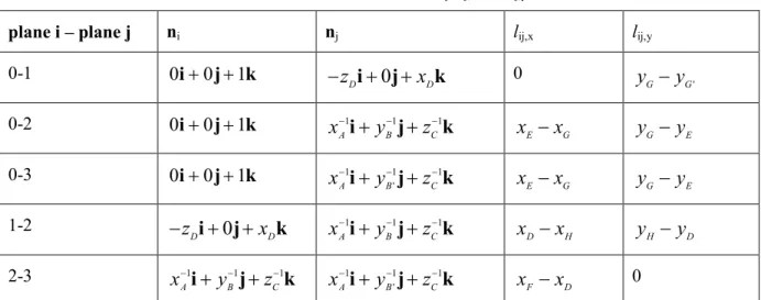
The design by the component method requires the simulation of the joint by means of a series of different components. Each component was represented by an elastic spring characterised by a specific stiffness and strength, as highlighted in Figure . The appropriate coupling in parallel and series of these springs provides the global stiffness of the joint. As far as the global connection strength was concerned, different failure mechanisms were identified, the minimum value of failure loads being the design resistance of the connection. The components considered are reported in Table .

Figure 11. A steel-concrete composite bolted beam-to-column joint and its mechanical model.

The composite column was assumed to be infinitely rigid during the application of the component method. In greater detail, beam-to-column joints were rigid and full-strength joints. The joint overstrength can be guaranteed by the following relation

, 1.1 , ,

j Rd ov b pl Rd

M ≥ ⋅

γ

⋅M

where Mj,Rd defines the resisting moment of the beam-to-column joint assumed to be full strength and

Mb,pl,Rd represents the resisting moment of the adjacent composite beam.

Table 4. Joint components relevant to sagging and hogging bending moment

Sagging Bending Moment Hogging Bending Moment

Concrete slab in compression

Upper horizontal plate in compression Vertical plate in bending

Lower horizontal plate in tension

Longitudinal rebars in tension Upper horizontal plate in tension Vertical plate in bending

Lower horizontal plate in compression

References

[1] Anderson D (ed). COST C1 - Composite steel-concrete joints in frames for buildings: Design provisions. Brussels – Luxembourg, 1999.

[2] Eurocode 3: Design of steel structures, Part 1-1: General rules and rules for buildings. EN 1993-1-1, Brussels, 2005.

[3] Eurocode 3: Design of steel structures - Part 1-6: Strength and Stability of Shell Structures. EN 1993-1-6, Brussels, 2007.

[4] Pappa, P., and Karamanos, S. A., “Buckling of High-Strength Steel CHS Tubular Members under

axial compression and bending,” 14th International Symposium on Tubular Structures, Paper No. 104, London, UK, 2012.

15 [5] Pournara A.E., Karamanos S.A., Ferino J., Lucci A., “Strength and stability of high-strength steel

tubular beam-columns under compressive loading,” 14th International Symposium on Tubular Structures, Paper No. 103, London, UK, 2012.

[6] Eurocode 3: Design of steel structures, Part 1-2: General rules - Structural fire design. EN 1993-1-2, Brussels, 2004.

[7] Eurocode 3: Design of steel structures - Part 1-8: Design of joints. EN 1993-1-8, Brussels, 2003. [8] Eurocode 4: Design of composite steel and concrete structures, Part 1-2: General rules - Structural

fire design. EN 1994-1-1, Brussels, 2004.

[9] Guisse S, Vandegans D, Jaspart JP. Application of the component method to column bases – experimentation and development of a mechanical model for characterization. Research Centre of the Belgian Metalworking Industry, 1996.

[10] Eurocode 4: Design of composite steel and concrete structures, Part 1-1: General rules and rules for buildings. EN 1994-1-1, Brussels, 2004.

[11] Hoang VL et al. Field of application of high strength steel circular tubes for steel and composite columns from an economic point of view. Journal of Constructional Steel Research, (67):1001-1021, 2011.

16

Appendix A:

s

tatic column base A1. Introduction

This appendix details Section 4.1.3, on:

- the assembly of the component (detail of the interaction equations); - the calculation of the “concrete in compression” component;

- the calculation of the “end plate in bending, bolts in tension” component.

A2. Notices

Geometric dimensions of the column base are indicated on Fig.A1.

'

2 * 0.8 * 2

d

= +

d

a

;

s

,

= −

s

0.8 2

a

Fig.A1. Geometric dimensions of the static column base

17

Fig.A2. Column base - Assembly of plate, anchor bolts and concrete block components

The applied moment (MEd) and axial force (NEd) are equilibrium by the “concrete in compression” (fi) and “plate in bending, bolts in tension” (Ft) components (Fig.A2). The force Ft varies according to the width of the compression zone as the show on Fig.A2, this relation is proposed in [2]. How to obtain fi (concrete in compression) and Ftmax (plate in bending, bolts intension) are presented in Section A.4 and A.5, respectively. When fi and Ft are determined, the interaction curve of bending moment and axial force can be written as Eqs. (A1) and (A2):

, Rd c j t x N = A f −F ; _(A1) 1 2 , ( ) Rd j t x M = S −S f +F y. _(A2) with 1 2 ( ) c eff A =A − A −A 2 2 1 2 ( ) eff A =

π

r −r 2 1 1 ( / 2 1 sin 1cos )1 A =r

π

−

θ

−

θ

θ

2 2 2( / 2 2 sin 2cos 2) A =r

π

−

θ

−

θ

θ

3 3 1 1 1 2 cos 3 S = r

θ

3 3 2 2 2 2 cos 3 S = r

θ

,

0

if

2.5 (

) /

if

0.6

x<z

if

0.6

t x t t

x

z

F

F z

x

z

z

F

x

z

≥

=

−

≤

<

1

z

= +

r

y

18 2 2 1 1 2 1 1 2 2 2 1 1 2 2 2 2 1 1

sin

arctan

if

( sin

)

0

( sin

)

/ 2

if

( sin

)

0

r

r

r

r

r

r

r

θ

_θ

θ

θ

π

θ

−

>

−

=

−

≤

;

Let vary from to , using Eqs. (A1) and (A2), it is possible to depict the interaction curve (curve ABC on Fig.A3).

Fid.A3. Interaction curve for plate in bending, bolts in tension and concrete in compression

A4. “Concrete in compression” component [2]

Fig.A4. Effective plate

Due to the volume effect, the strength of the concrete in compression should be multiplied by the “concentration ratio”. On the other hand, due to the flexibility of the end plate, the concrete reaction applies only within a zone defined by an effective rigid plate, see Fig.A4.

The concentration ratio is calculated Eq.A3 as follow:

eff eff j B L k bh = (A3)

with Beff and Leff are the effective dimensions of the concrete block and they are determined by Eq.A4:

1 min( 2 ; 5 ; ; 5 ) eff p eff B = b+ B b h +H L ≥b 1 min( 2 ; 5 ; ; 5 ) eff p eff L = h+ L h h +H B ≥h (A4)

The admissible stress in the concrete block can reach the value, Eq.(A5): 1

19 ck j j j c f f

β

k

γ

= (A5)

with

β

_j =2 / 3;

f

ckis the characteristic strength of the concrete in compression;

γ

cis the partial safety

factor for the concrete.

The equivalent rigid plate (Fig.A4) is a ring that is determined through the parameter c (Fig.A4) by Eq.A6: 0 3 yp p j M f c t f

γ

= (A6)

where tp is the base plate thickness; fyp is the yielded strength of the base plate;

γ

M0is the partial safety

factor for the steel.

A5. The “end plate in bending, bolts in tension” component

A5.1. Development

This component is developed by using limit analysis on the column base where rigid-plastic material concept is used for the end plate and the bolts while the foundation is considered as rigid behaviour (Fig.A5). As present in Section 4.1.3, seven (7) licit mechanisms are considered (Fig.A6). However, only the study on the mechanisms “e” and “f” (Fig.A6) are presented herein, the calculation of the other mechanisms can be found in the literature, e.g [1], [3].

Fig.A5. Column base in limit analysis

20

Fig.A7. Mechanism “e” family

Fig.A7 details the geometries of the mechanism “e”. In fact, this is a family of mechanism where the difference of its members is the position of point B on the y axe (or position of the point A on x axe). Six (6) yield lines are formed and the end plate is devised into four (4) rigid planes: plane o (ABB’), plane 1 (DBB’), plane 2 (ABD), and plane 3 (AB’D). It needs to find the optimal mechanism (real mechanism) in this family, on the other word, it should find the optimal position of point B (or A). The virtual work principle is applied and the main formulas are presented in Tables A.1, A.2 and A.3 below.

Table A.1: Main equations for limit analysis of the investigated structure

Equation Eq. number Indication

E I

W

=

W

(A7) Virtual work principle

E

W

=

M

ϕ

(A8) External work

I p ij ij

W =m

∑

θ

l (A9) Internal work 2

/ 4

p p y

m =t f (A10) Unit plastic moment of the end plate

2 2 , , ij ij x ij y

l

=

l

+

l

(A11) Length of the yield line ij between plane i and plane j; with lij x, , ,

ij y

l are the components of l_ijon the x and y axis, respectively.

i j ij i j

θ

≈ × • n n n n

(A12) Rotation of the yield line ij between plane i and plane j; with ni and nj are the normal vectors of the plane i and plane j respectively.

21

Table A.2: determination of ni, nj, lij,x and lij,y

plane i – plane j ni nj lij,x lij,y

0-1 0i+0j+1k

−

z

D

i

+

0

j

+

x

D

k

0

y

G

−

y

G' 0-2 0i+0j+1k 1 1 1 A B C

x

−

i

+

y

−

j

+

z

−

k

x

E

−

x

G

y

G

−

y

E 0-3 0i+0j+1k 1 1 1 ' A B C

x

−

i

+

y

−

j

+

z

−

k

x

_E

−

x

_G

y

G

−

y

E 1-2

₀

D D

z

x

−

i

+

j

+

k

1 1 1 A B C

x

−

i

+

y

−

j

+

z

−

k

x

_D

−

x

_H

y

H

−

y

D 2-3 1 1 1 A B C

x

−

i

+

y

−

j

+

z

−

k

1 1 1 ' A B C

x

−

i

+

y

−

j

+

z

−

k

x

_F

−

x

_D 0

All above geometric quantities (in Table A.2) can be written under the functions of yB, as the present in Table A3.

Table A3: the coordinates of the point A, B, C, D, E, F, G, H following yB.

Quantities Equation xD

0.5 {1 cos[2

'

(

'

/(2

)}/ cos{2

[

'

/(2

)]}

D B B

x

=

d

+

artg d

y

artg d

y

xA

[(

'

/ 2) /(

/ 2)]

A B B

x

=

y

y

+

d

y

−

e

zD D D

z

=

ϕ

x

yB’ ' B B

y

=

y

zc

/(

)

C A D A D

z

=

x x

x

−

x

yG

/ 2

G

y

=

b

yG’ '

/ 2

G

y

= −

b

XE ' , 1 E

x

=

d

+ +

n

e

xG

[1

/(2

)]

G A B

x

=

x

−

b

y

yE ' , 1

[

(

)]/

E B A A

y

=

y x

−

d

+ +

n

e

x

xH

(

/ 2) /

H D B B

x

=

x

y

−

b

y

yH

/ 2

H

y

=

b

xF F E

x

=

x

22 Now, the virtual work principle of Eq.(A7) can be written as:

M

=

W y

_I

(

_B

)

.

And the optimal mechanism is found by solving the following, Eq.A13:

0 optimal mechanism i B dW dy = → . (A13)

In principle, the analytical solution of Eq.(A13) can be obtain, however its explicit form is quite complicated. Therefore, for the reason of practical application, in this work, Eq.(A13) is solved by the numerical way. The moment (Mp5 in Table 3) is written as Mp5 =

α

1bmp and the coefficient α1 can be

numerically determined. The geometric dimensions of the end plate, the tube and the bolt position are varied such that almost practical cases may be covered: '

/ 1, 2 2, 0 b d = ÷ ;h b/ =1, 0 1, 6÷ ; , 2 2 , 1 2 /( ) 0, 3 0, 7 m e e m

β

= + + = ÷ (β concerns the bolt position). The bolts are supposed be on the diagonal of the end plate. α1 is given in Table A4.

The same analysis (from the basis equations to the numerical calculations) are carried out for the mechanism “f “ and the coefficients α2 and α3 (see Table A3) are given in Tables A5 and A6, respectively.

Noting that in mechanisms “e” and “f” the prying force is taken into account. If the prying force is not considered, the mechanism “f” is modified and the coefficient α4 (see Table A7) can be obtained and given in Table A7.

23

Table A4: coefficient α1

β h/b b/d’ 1,2 1,3 1,4 1,5 1,6 1,7 1,8 1,9 2,0 0,3 1,0 19,373 17,194 15,561 14,277 13,234 12,373 11,640 11,005 10,467 1,1 18,447 16,512 15,019 13,833 12,861 12,050 11,259 10,494 9,849 1,2 17,694 15,939 14,561 13,375 12,181 11,214 10,415 9,740 9,167 1,3 17,078 15,311 13,618 12,306 11,259 10,406 9,695 9,094 8,581 1,4 15,981 14,029 12,556 11,402 10,475 9,714 9,077 8,538 8,075 1,5 14,654 12,953 11,653 10,628 9,800 9,116 8,543 8,055 7,634 1,6 13,537 12,036 10,880 9,962 9,216 8,598 8,076 7,631 7,247 0,4 1,0 14,222 12,660 11,492 10,576 9,836 9,226 8,708 8,264 7,881 1,1 13,543 12,151 11,089 10,247 9,560 8,990 8,500 8,080 7,717 1,2 12,974 11,721 10,745 9,962 9,319 8,780 8,316 7,849 7,418 1,3 12,505 11,352 10,449 9,714 8,988 8,347 7,813 7,362 6,976 1,4 12,110 11,040 9,959 9,093 8,397 7,825 7,347 6,942 6,594 1,5 11,535 10,256 9,280 8,511 7,888 7,375 6,944 6,576 6,260 1,6 10,694 9,567 8,699 8,009 7,448 6,983 6,591 6,257 5,967 0,5 1,0 11,139 9,943 9,052 8,357 7,798 7,339 6,950 6,619 6,332 1,1 10,601 9,537 8,732 8,096 7,581 7,151 6,786 6,475 6,201 1,2 10,144 9,192 8,457 7,869 7,387 6,982 6,638 6,344 6,083 1,3 9,766 8,894 8,215 7,668 7,214 6,832 6,506 6,224 5,975 1,4 9,441 8,640 8,006 7,491 7,062 6,698 6,314 5,989 5,709 1,5 9,166 8,420 7,823 7,246 6,747 6,334 5,988 5,693 5,439 1,6 8,930 8,091 7,395 6,842 6,392 6,018 5,704 5,435 5,203 0,6 1,0 9,087 8,133 7,426 6,878 6,439 6,081 5,778 5,522 5,299 1,1 8,639 7,796 7,161 6,663 6,261 5,925 5,643 5,402 5,192 1,2 8,259 7,507 6,931 6,472 6,097 5,785 5,521 5,291 5,094 1,3 7,939 7,258 6,728 6,302 5,952 5,659 5,408 5,191 5,002 1,4 7,666 7,041 6,551 6,153 5,824 5,545 5,306 5,100 4,919 1,5 7,432 6,853 6,394 6,020 5,708 5,443 5,215 5,018 4,843 1,6 7,229 6,689 6,257 5,902 5,604 5,351 5,113 4,888 4,694 0,7 1,0 7,620 6,837 6,264 5,821 5,469 5,182 4,940 4,738 4,561 1,1 7,238 6,552 6,039 5,639 5,316 5,050 4,827 4,635 4,470 1,2 6,913 6,304 5,840 5,474 5,177 4,929 4,720 4,540 4,384 1,3 6,635 6,088 5,665 5,327 5,050 4,819 4,622 4,452 4,305 1,4 6,397 5,900 5,510 5,197 4,938 4,720 4,533 4,373 4,232 1,5 6,193 5,735 5,373 5,080 4,836 4,630 4,453 4,300 4,165 1,6 6,016 5,591 5,252 4,976 4,745 4,549 4,380 4,233 4,105

Table A5: coefficient α2

β h/b b/d’ 1,2 1,3 1,4 1,5 1,6 1,7 1,8 1,9 2 1,0 4,981 4,508 4,170 3,916 3,718 3,559 3,428 3,318 3,225 1,1 4,716 4,312 4,017 3,792 3,614 3,470 3,350 3,250 3,164 1,2 4,482 4,132 3,872 3,671 3,511 3,381 3,272 3,179 3,100 1,3 4,276 3,969 3,739 3,558 3,413 3,294 3,194 3,109 3,036 1,4 4,093 3,822 3,616 3,453 3,321 3,212 3,120 3,042 2,974 1,5 3,932 3,690 3,504 3,356 3,235 3,135 3,050 2,977 2,914 1,6 3,788 3,571 3,402 3,266 3,156 3,063 2,984 2,916 2,857

24

Table A6: coefficient α3

β h/b b/d’ 1,2 1,3 1,4 1,5 1,6 1,7 1,8 1,9 2,0 0,3 1,0 0,515 0,480 0,447 0,418 0,392 0,371 0,350 0,334 0,317 1,1 0,528 0,489 0,455 0,426 0,402 0,378 0,359 0,340 0,324 1,2 0,535 0,498 0,464 0,434 0,409 0,385 0,365 0,347 0,330 1,3 0,545 0,505 0,472 0,441 0,415 0,391 0,371 0,352 0,336 1,4 0,552 0,511 0,477 0,447 0,421 0,397 0,376 0,357 0,340 1,5 0,559 0,518 0,483 0,453 0,425 0,402 0,380 0,362 0,344 1,6 0,565 0,523 0,488 0,457 0,430 0,406 0,385 0,365 0,348 0,4 1,0 0,441 0,412 0,383 0,358 0,336 0,318 0,300 0,286 0,271 1,1 0,453 0,419 0,390 0,365 0,344 0,324 0,308 0,291 0,278 1,2 0,459 0,427 0,397 0,372 0,350 0,330 0,313 0,298 0,283 1,3 0,467 0,433 0,404 0,378 0,356 0,335 0,318 0,302 0,288 1,4 0,474 0,438 0,409 0,383 0,361 0,341 0,322 0,306 0,292 1,5 0,479 0,444 0,414 0,388 0,365 0,345 0,326 0,310 0,295 1,6 0,484 0,448 0,418 0,392 0,369 0,348 0,330 0,313 0,298 0,5 1,0 0,368 0,343 0,319 0,298 0,280 0,265 0,250 0,238 0,226 1,1 0,377 0,349 0,325 0,304 0,287 0,270 0,256 0,243 0,232 1,2 0,382 0,356 0,331 0,310 0,292 0,275 0,261 0,248 0,236 1,3 0,389 0,361 0,337 0,315 0,297 0,279 0,265 0,252 0,240 1,4 0,395 0,365 0,341 0,319 0,301 0,284 0,269 0,255 0,243 1,5 0,399 0,370 0,345 0,323 0,304 0,287 0,272 0,258 0,246 1,6 0,403 0,374 0,349 0,327 0,307 0,290 0,275 0,261 0,248 0,6 1,0 0,294 0,274 0,255 0,239 0,224 0,212 0,200 0,191 0,181 1,1 0,302 0,279 0,260 0,243 0,229 0,216 0,205 0,194 0,185 1,2 0,306 0,285 0,265 0,248 0,234 0,220 0,209 0,198 0,188 1,3 0,312 0,289 0,269 0,252 0,237 0,223 0,212 0,201 0,192 1,4 0,316 0,292 0,273 0,256 0,240 0,227 0,215 0,204 0,194 1,5 0,319 0,296 0,276 0,259 0,243 0,230 0,217 0,207 0,197 1,6 0,323 0,299 0,279 0,261 0,246 0,232 0,220 0,209 0,199 0,7 1,0 0,221 0,206 0,192 0,179 0,168 0,159 0,150 0,143 0,136 1,1 0,226 0,210 0,195 0,182 0,172 0,162 0,154 0,146 0,139 1,2 0,229 0,213 0,199 0,186 0,175 0,165 0,156 0,149 0,141 1,3 0,234 0,216 0,202 0,189 0,178 0,168 0,159 0,151 0,144 1,4 0,237 0,219 0,205 0,192 0,180 0,170 0,161 0,153 0,146 1,5 0,240 0,222 0,207 0,194 0,182 0,172 0,163 0,155 0,148 1,6 0,242 0,224 0,209 0,196 0,184 0,174 0,165 0,157 0,149

25

Table A7: coefficient α4

β h/b b/d’ 1,2 1,3 1,4 1,5 1,6 1,7 1,8 1,9 2 0,3 1,0 12,601 10,931 9,729 8,820 8,110 7,531 7,057 6,662 6,321 1,1 11,539 10,116 9,072 8,273 7,640 7,100 6,640 6,256 5,930 1,2 10,625 9,400 8,475 7,715 7,114 6,625 6,221 5,882 5,593 1,3 9,836 8,694 7,842 7,181 6,653 6,222 5,864 5,561 5,303 1,4 9,036 8,053 7,310 6,728 6,261 5,877 5,556 5,284 5,051 1,5 8,371 7,513 6,858 6,342 5,924 5,579 5,290 5,044 4,832 1,6 7,810 7,054 6,471 6,008 5,632 5,320 5,057 4,833 4,639 0,4 1,0 9,856 8,616 7,724 7,051 6,524 6,097 5,746 5,454 5,203 1,1 9,085 8,027 7,252 6,658 6,188 5,806 5,491 5,224 4,997 1,2 8,417 7,504 6,825 6,299 5,879 5,519 5,215 4,960 4,742 1,3 7,840 7,045 6,431 5,934 5,537 5,213 4,943 4,715 4,520 1,4 7,327 6,588 6,029 5,592 5,240 4,951 4,709 4,504 4,328 1,5 6,825 6,180 5,688 5,299 4,984 4,724 4,506 4,320 4,160 1,6 6,402 5,833 5,394 5,046 4,762 4,527 4,329 4,159 4,013 0,5 1,0 8,219 7,236 6,530 5,996 5,579 5,243 4,966 4,735 4,537 1,1 7,619 6,780 6,165 5,695 5,323 5,021 4,772 4,561 4,381 1,2 7,097 6,373 5,834 5,417 5,085 4,813 4,586 4,395 4,230 1,3 6,645 6,013 5,537 5,165 4,866 4,614 4,397 4,213 4,056 1,4 6,252 5,695 5,267 4,916 4,633 4,400 4,206 4,041 3,899 1,5 5,904 5,386 4,990 4,678 4,425 4,216 4,040 3,890 3,761 1,6 5,562 5,105 4,752 4,472 4,244 4,055 3,895 3,758 3,640 0,6 1,0 7,134 6,322 5,739 5,298 4,954 4,678 4,450 4,259 4,097 1,1 6,646 5,952 5,444 5,057 4,750 4,501 4,295 4,121 3,973 1,2 6,221 5,622 5,177 4,832 4,557 4,333 4,146 3,987 3,852 1,3 5,852 5,329 4,935 4,627 4,379 4,176 4,005 3,860 3,735 1,4 5,529 5,068 4,717 4,440 4,216 4,030 3,872 3,733 3,613 1,5 5,246 4,836 4,521 4,266 4,053 3,878 3,730 3,604 3,495 1,6 4,998 4,622 4,326 4,091 3,900 3,740 3,606 3,491 3,391 0,7 1,0 6,361 5,670 5,175 4,803 4,511 4,276 4,083 3,921 3,784 1,1 5,954 5,363 4,932 4,603 4,342 4,131 3,956 3,809 3,683 1,2 5,598 5,088 4,709 4,416 4,182 3,991 3,832 3,698 3,582 1,3 5,287 4,842 4,506 4,244 4,033 3,860 3,715 3,591 3,485 1,4 5,015 4,622 4,323 4,086 3,895 3,737 3,604 3,491 3,393 1,5 4,776 4,426 4,157 3,943 3,769 3,624 3,501 3,397 3,304 1,6 4,564 4,251 4,007 3,812 3,653 3,515 3,399 3,299 3,213 A5.2. Validation

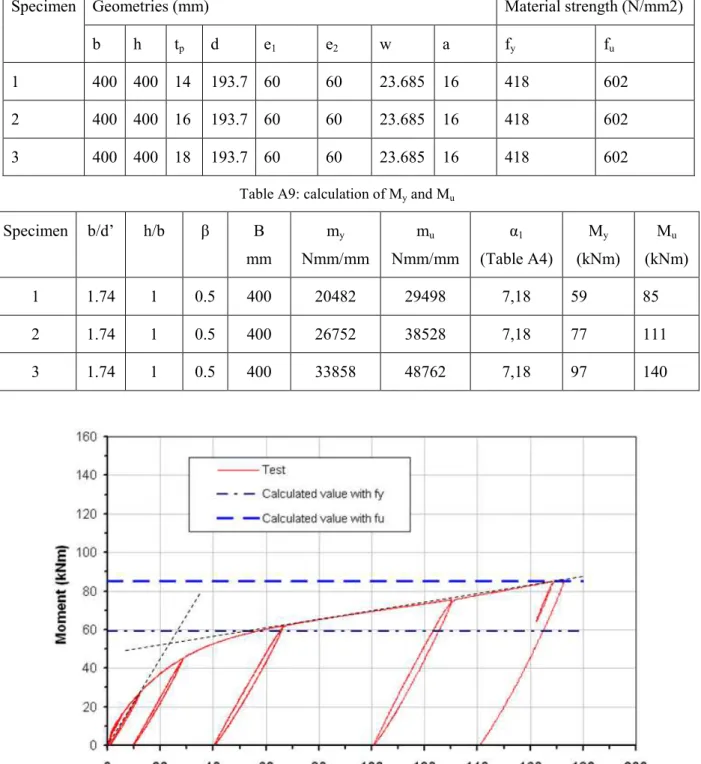
The results of the above development are compared with the experimental tests within WP3 (See Deliverable D3). Three specimens with the variation of the end plate thickness were tested with the main parameters of the specimens are presented in Table A8. The calculations using the present development of moments My and Mu (by using fy and fu respectively) are summarized in Table A9. The mechanism “e” occurs according to both analytical and experimental investigations. The Figs.A8-A10 shows that the present results are in agreement with the experimental ones.

26

Table A8: Geometries and material of the specimens (the symbols can be found on Fig.A1)

Specimen Geometries (mm) Material strength (N/mm2)

b h tp d e1 e2 w a fy fu

1 400 400 14 193.7 60 60 23.685 16 418 602

2 400 400 16 193.7 60 60 23.685 16 418 602

3 400 400 18 193.7 60 60 23.685 16 418 602

Table A9: calculation of My and Mu

Specimen b/d’ h/b β B mm my Nmm/mm mu Nmm/mm α1 (Table A4) My (kNm) Mu (kNm) 1 1.74 1 0.5 400 20482 29498 7,18 59 85 2 1.74 1 0.5 400 26752 38528 7,18 77 111 3 1.74 1 0.5 400 33858 48762 7,18 97 140

27

Fig.A9. Comparison for specimen 2

Fig.A10. Comparison for specimen 3

A.6. Conclusion

The resistance determination of the column base by using the component methods is presented. In particular, based on the limit analysis, the practical calculation for the “plate in bending, bolts in tension” component of the column base is proposed. The results are in agreement with the experimental one.

References for Appendix A

[1] Eurocode 3: Design of steel structures - Part 1-8: Design of joints. EN 1993-1-8, Brussels, 2003. [2] Guisse S, Vandegans D, Jaspart JP. Application of the component method to column bases –

experimentation and development of a mechanical model for characterization. Research Centre of the Belgian Metalworking Industry, 1996.

[3] Jaspart JP. Recent advances in the field od steel joints column bases and further configurations for beam-to-column joints and beam splices. Agregation Thesis, University of Liege, 1997.

28

Appendix B: Through plate of static joint B1. Introduction

This appendix details Section 5.1.3, on the development for the through plate of the static joint.

B2. Notices (Fig.B1)

t: thickness of the plate; h: height of the plate;

b: width of the plate part outside the tube; D: inside diameter of the tube;

FEd: design value of the horizontal component of the load; VEd: design value of the vertical component of the load; α: load direction;

E: Young modulus; υ: Poisson ratio.

Fig.B1. Beam-to-column joints - through plate component

B3. General considerations and hypotheses

Fig.B2 describes the buckling mode of the whole joint while the buckling mode of the through plate is shown on the Fig.B3.

29

Fig.B2. Buckling mode of joint

Fig.B3. Buckling mode of through plate

For the simplification reason, the through plate is devised into two parts, inside part (inside the column) and outside parts (outside the column) with the boundary and loading condition as the show on Fig.B3. The buckling theory of plate is applied to study the strength of each part.

30

Fig.B4. modelling of boundary and loading for the through plate

B4. Design of the through plate

Using the buckling theory of plates, the buckling stresses of the inside and outside parts can be written by Eqs.(B1) and (B2) as follows:

2 2 , 1 2 12(1 ) c ou E t b

π

σ

µ

ν

  = _{ } −   ; (B1) 2 2 , 2 2 12(1 ) c in E t h

π

σ

µ

ν

  = _{ } −   . (B2)

The coefficients µ1 and µ1 in Eqs. (B1) and (B2) are used to take into account boundary condition, loading condition, plasticity and initial imperfection. In this work, these coefficients are determined by the numerical analysis, as Eqs.(B3) and (B4):

2 2 1 ( , ) / 2 12(1 ) c ou numerical E t b

π

µ

σ

ν

 _{ }  = _{   } −    ; (B3) 2 2 2 ( , ) / 2 12(1 ) c in numerical E t h

π

µ

σ

ν

 _{ }  = _{   } −    , (B4)

with σnumerical is calculated by LAGAMINE (a nonlinear finite element code developed in University of Liege) considering the boundary condition, the loading, the plasticity and the initial imperfection, as the description on Figs.B5 and B6. The detail on the numerical strategy and its validation are presented in WP5 (see Deliverable D5). The parametric study (the geometric dimensions of the plate are varied such that almost practical case can be coved) is performed, and the corresponding values of µ1 and µ1 are obtained.

31

Fig.B5. modeling of the initial imperfection for the plate

Fig.B6. Material modelling in the numerical analysis

Finally, the safety verification of the through plate may be performed by the following formula: 2 2 1 2 1 2 2 2 1 2 2 / ; 12(1 ) 4 4 / . 12(1 ) Ed M Ed Ed M V E t th b F V b E t th th h

π

κµ

γ

υ

π

µ

γ

υ

 _{ } ≤  ₋          _{+ ≤}    _{−  }  (B5)

with γM1 is the partial factor according to EN1993-1-1 [1]; κ= 1.0 for the rectangular outside part and κ = 0.9 for the triangular outside part; µ1 and µ2 are given in Tables B1 and B2. Three loading types in Table B2 is shown on Fig.B7, in which σmax and σmin are calculated as follows (Eq.(B6)):

max 2 min 2 4 4 4 4 ; Ed Ed Ed Ed V b F V b F th th th th

σ

= −

σ

= + (B6) .

32

Fig.B7: loading type for the inside part of the plate

Noting that the value of µ1 and µ2 given in Tables 1 and 2 are only validated for S355 steel.

Table B1: Buckling stress factor for outside plate (µ1)

Geometries Load direction α (in degree)

h/b t/b α=90 α=60 α=45 α=30 α=15 0,6 0,505 0,1686 0,1591 0,1718 0,1654 0,0632 0,075 0,1027 0,0887 0,0871 0,0840 0,0397 0,100 0,0763 0,0610 0,0589 0,0531 0,0302 0,125 0,0661 0,0475 0,0433 0,0381 0,0213 0,150 0,0546 0,0402 0,0343 0,0304 0,0185 0,8 0,050 0,2455 0,2518 0,2487 0,1654 0,0717 0,075 0,1467 0,1343 0,1308 0,1080 0,0465 0,100 0,1027 0,0902 0,0844 0,0677 0,0337 0,125 0,0801 0,0672 0,0620 0,0488 0,0255 0,150 0,0699 0,0543 0,0492 0,0384 0,0225 1,0 0,050 0,3151 0,3246 0,2750 0,1675 0,0790 0,075 0,1820 0,1758 0,1636 0,1115 0,0525 0,100 0,1263 0,1117 0,0985 0,0778 0,0370 0,125 0,0908 0,0812 0,0742 0,0591 0,0293 0,150 0,0744 0,0640 0,0582 0,0464 0,0260 1,2 0,050 0,3762 0,3857 0,2792 0,1739 0,0843 0,075 0,2042 0,2039 0,1964 0,1230 0,0568 0,100 0,1317 0,1263 0,1142 0,0829 0,0419 0,125 0,0961 0,0893 0,0807 0,0637 0,0331 0,150 0,0715 0,0691 0,0624 0,0520 0,0288 1,4 0,050 0,4194 0,4278 0,2792 0,1770 0,0875 0,075 0,2217 0,2535 0,1789 0,1190 0,2869 0,100 0,1386 0,1374 0,1191 0,0844 0,0436 0,125 0,0993 0,0943 0,0859 0,0658 0,0348 0,150 0,0786 0,0713 0,0654 0,0546 0,0304

33

Table B2: Buckling stress factor for inside plate (µ2)

Geometries Load type (Fig.B7)

D/b t/h type 1 type 2 type 3

1,00 0,050 1,0875 0,7819 0,4805 0,075 0,5620 0,4409 0,2779 0,100 0,2792 0,2761 0,1710 0,125 0,1794 0,1794 0,1145 0,150 0,1246 0,1246 0,0826 1,15 0,050 1,0474 0,6997 0,4173 0,075 0,5364 0,4146 0,2785 0,100 0,2792 0,2632 0,1644 0,125 0,1794 0,1794 0,1111 0,150 0,1246 0,1246 0,0795 1,33 0,050 1,0495 0,6006 0,4152 0,075 0,5208 0,3828 0,3072 0,100 0,2792 0,2487 0,1617 0,125 0,1794 0,1731 0,1146 0,150 0,1246 0,1246 0,0846 1,67 0,050 1,0116 0,4636 0,2466 0,075 0,5358 0,3335 0,1886 0,100 0,2792 0,2358 0,1370 0,125 0,1794 0,1794 0,1196 0,150 0,1246 0,1208 0,0731 2,00 0,050 0,9800 0,3498 0,1834 0,075 0,5189 0,2760 0,1636 0,100 0,2792 0,2044 0,1175 0,125 0,1794 0,1511 0,0924 0,150 0,1246 0,1133 0,0729 B5. Conclusions

The formulas for design of the through plate of the static joints are proposed. These formulas are based on the elastic plate buckling formulation while the plasticity, the boundary conditions, the loading ways and the initial imperfection are taken into account by numerical analysis. The parametric study is also carried out on the geometric dimensions of the plate.

References for Appendix B

[1] Eurocode 3: Design of steel structures, Part 1-1: General rules and rules for buildings. EN 1993-1-1, Brussels, 2005.

34

Appendix C: Cross-Sectional Strength of high-strength steel tubular members

EN 1993-1-1 provisions classify high-strength steel CHS members with relatively low values of D/t ratio as Class 3 or 4, so that their strength is based on elastic behavior only, neglecting their capability of sustaining inelastic deformation before a maximum resistance is reached. To investigate the applicability of the above classification, a special-purpose numerical technique is employed to examine the resistance against local buckling of high-strength steel seamless tubular members with significant thickness, that exhibit local buckling in the plastic regime under axial compression and bending. The numerical technique employs large inelastic strains, accounts for the presence of initial imperfections/residual stresses, and is capable of describing deformation and buckling of tubular cross-sections well beyond yielding of the steel material. Imperfections and residual stresses from real measurements are used. Numerical results are presented in terms of both the ultimate load and the deformation capacity of typical cross-sections, and are compared with available experimental data. The results aim at evaluating the applicability of EN 1993-1-1 for cross-sectional classification of high-strength steel CHS seamless tubular members.

C1-Introduction

High-strength steel CHS tubes are becoming popular in a variety of structural engineering applications, such as tubular columns of building systems or members of tubular lattice structures. The principal characteristic of these steel products, with respect to CHS tubes of normal steel grades, is the elevated yield stress value, which implies increased ultimate capacity, resulting in a good relationship between weight and strength. They can also be efficient in cases where space occupancy becomes a critical design criterion.

According to current design practice, the ultimate capacity of steel sections under axial and bending loads depends primarily on whether the section is classified as “compact” or “non-compact”, i.e. on the ability of the cross-section to sustain significant inelastic deformation before failure in the form of local buckling. In particular, the provisions of EN 1993-1-1 standard specify four (4) cross-sectional classes, where Class 4 corresponds to thin-walled sections, which are able to sustain axial/bending load only in the elastic range, Class 1 includes thick-walled sections that are able to deform well into the plastic regime, without exhibiting local buckling, and Classes 2 and 3 refer to intermediate type of structural behavior. For the case of CHS tubular members, classification in EN 1993-1-1 is based on the value of the diameter-to-thickness ratio, as well as on the value of the material yield stress, as shown in the second column of Table 1. The same classification is also adopted by the CIDECT guidelines [16] for hollow section stability, whereas similar provisions for cross-sectional classification on CHS members can be found in other specifications (e.g. AISC, API RP2A – LRFD).

The above classification provisions do not cover the case of high-strength steel CHS tubular members. In the EN 1993 steel design framework, a new standard has been issued EN 1993-1-12 to specify the applicability of the other EN 1993-1-xx standards in high-strength steel applications. According to EN 1993-1-12, the EN 1993-1-1 classification provisions may be applied for high-strength steel members as well. However, the existing classification for CHS tubular members appears to be quite penalizing for high-strength steel tubular members; one can readily obtain from Table 1 that CHS sections with

D t= 35 and

σ

_Y=690 MPa, are classified as Class 4 sections, which implies a low ultimate capacity, within the elastic range.

The key issue in the above classification of CHS members is their cross-sectional strength, mainly in terms of local buckling, which constitutes a shell-buckling problem in the inelastic range. Inelastic buckling of relatively thick-walled steel cylinders under compressive loads has been the issue of significant research. Experimental observations ([4] and [13]) have been shown that under pure axial compression, thick-walled cylinders – in contrast with thin-walled ones – do not fail abruptly, but one can observed significant wall wrinkling before an ultimate load occurs. Analytically, a main challenge for solving this problem has been the combination of structural stability principles with inelastic multi-axial material behavior. In particular, it has been shown that buckling predictions depend on the choice of plasticity theory [17]. For a detailed presentation of metal cylinder buckling behavior under uniform axial compression, the reader is referred to the recent papers ([2] & [3]).

In addition to uniform axial compression, bending buckling of tubular members has also received significant attention, motivated mainly by their use in pipeline applications. Experimental works indicated that failure of thick-walled tubes under bending is associated with tube wall wrinkling, has