Study of Schnyder Woods and Intersection Graphs

Texte intégral

(1)Study of Schnyder Woods and Intersection Graphs Daniel Gonçalves. To cite this version: Daniel Gonçalves. Study of Schnyder Woods and Intersection Graphs. Discrete Mathematics [cs.DM]. Université de Montpellier, 2018. �tel-02078613�. HAL Id: tel-02078613 https://hal-lirmm.ccsd.cnrs.fr/tel-02078613 Submitted on 25 Mar 2019. HAL is a multi-disciplinary open access archive for the deposit and dissemination of scientific research documents, whether they are published or not. The documents may come from teaching and research institutions in France or abroad, or from public or private research centers.. L’archive ouverte pluridisciplinaire HAL, est destinée au dépôt et à la diffusion de documents scientifiques de niveau recherche, publiés ou non, émanant des établissements d’enseignement et de recherche français ou étrangers, des laboratoires publics ou privés..

(2) Habilitation ` a diriger des recherches pr´esent´ee ` a ´ DE MONTPELLIER L’UNIVERSITE Ecole Doctorale I2S. STUDY OF SCHNYDER WOODS AND INTERSECTION GRAPHS. Daniel GONC ¸ ALVES. Jury : Therese Biedl - University of Waterloo (rapportrice) Victor Chepoi - Aix-Marseille Universit´ e (examinateur) ´ Eric Colin de Verdi` ere - CNRS, Universit´ e Paris-Est Marne-la-Vall´ ee (rapporteur) Stefan Felsner - Technische Universit¨ at Berlin (rapporteur) Christophe Fiorio - Universit´ e de Montpellier (examinateur) Dieter Rautenbach - Universit¨ at Ulm (examinateur). 24 Septembre 2018.

(3) Foreword This document is a long abstract of my research work on graph theory. This is an overview of my research in the last 10 years (posterior to my PhD), and summarizes seven selected papers (included in the appendix) which have been published or are submitted to international journals. It summarizes some results, gives ideas of the proof for some of them, and presents the context of the different topics together with some interesting open questions connected to them. This document is organized as follow. The first two chapters respectively deal with Schnyder woods (and their extension on higher genus surfaces), and with intersection representations of planar graphs. The third chapter is a research project for the 5-10 years to come. Finally in the appendix one can find the full length papers which include all the proofs 1 . To conclude, I would like to mention that these papers are the result of different collaborations and each result is then a collective work. I would like to thank all my co-authors as well as many more colleagues for many nice and exciting moments doing research (or doing other things). I also warmly thank the members of the jury (and in particular the reviewers) for kindly accepting to be a part of it, and for all the time spent on this.. 1. As we uniformized notations from different publications, some notations differ between the manuscript and the papers.. 2.

(4) Table des mati` eres 1. 2. 3. Schnyder Woods 1.1 Introduction . . . . . . . . . . . . . . . . . . . . . . 1.2 Toroidal Schnyder Woods . . . . . . . . . . . . . . . 1.3 Applications of Toroidal Schnyder Woods . . . . . . 1.3.1 Drawing Algorithm . . . . . . . . . . . . . . 1.3.2 Bijection & Encoding . . . . . . . . . . . . . 1.4 Extensions to (oriented) Surfaces with higher Genus 1.4.1 Angle labelings . . . . . . . . . . . . . . . . 1.4.2 Orientations of weak Schnyder woods . . . . 1.5 (0 mod 3)-Orientations . . . . . . . . . . . . . . . 1.5.1 Proof of Theorem 1.24 . . . . . . . . . . . .. . . . . . . . . . .. . . . . . . . . . .. . . . . . . . . . .. . . . . . . . . . .. . . . . . . . . . .. . . . . . . . . . .. . . . . . . . . . .. . . . . . . . . . .. . . . . . . . . . .. . . . . . . . . . .. . . . . . . . . . .. . . . . . . . . . .. . . . . . . . . . .. . . . . . . . . . .. . . . . . . . . . .. . . . . . . . . . .. . . . . . . . . . .. . . . . . . . . . .. . . . . . . . . . .. . . . . . . . . . .. . . . . . . . . . .. . . . . . . . . . .. . . . . . . . . . .. 5 5 6 8 8 10 14 16 18 19 20. Intersection Representations for Planar Graphs 2.1 Introduction . . . . . . . . . . . . . . . . . . . . . . . . . . . . . . . . 2.1.1 Pseudo-disks . . . . . . . . . . . . . . . . . . . . . . . . . . . 2.1.2 Pseudo-segments . . . . . . . . . . . . . . . . . . . . . . . . . 2.2 Representations by Homothetic Triangles . . . . . . . . . . . . . . . . 2.3 Primal-Dual representations with Triangles . . . . . . . . . . . . . . . . 2.4 1-String Representations . . . . . . . . . . . . . . . . . . . . . . . . . 2.4.1 Proof for 4-connected triangulations. . . . . . . . . . . . . . . 2.4.2 Proof in the general case . . . . . . . . . . . . . . . . . . . . . 2.4.3 Improvements for getting segment intersection representations . 2.5 L-Representations . . . . . . . . . . . . . . . . . . . . . . . . . . . . . 2.5.1 2-sided near-triangulations . . . . . . . . . . . . . . . . . . . . 2.5.2 Thick x-contact representations . . . . . . . . . . . . . . . . . 2.5.3 The x-intersection representations . . . . . . . . . . . . . . . .. . . . . . . . . . . . . .. . . . . . . . . . . . . .. . . . . . . . . . . . . .. . . . . . . . . . . . . .. . . . . . . . . . . . . .. . . . . . . . . . . . . .. . . . . . . . . . . . . .. . . . . . . . . . . . . .. . . . . . . . . . . . . .. . . . . . . . . . . . . .. . . . . . . . . . . . . .. . . . . . . . . . . . . .. . . . . . . . . . . . . .. 25 25 25 27 29 33 35 35 37 39 40 40 41 43. Research Project 3.1 Schnyder woods in higher genus . . . . . . . . . 3.2 Intersection graphs on surfaces . . . . . . . . . . 3.3 Slope constraints for segment intersection graphs 3.4 Extensions to Rd through Simplicial Complexes .. . . . .. . . . .. . . . .. . . . .. . . . .. . . . .. . . . .. . . . .. . . . .. . . . .. . . . .. . . . .. . . . .. 47 47 48 49 49. . . . .. . . . .. . . . .. . . . .. . . . .. . . . .. . . . .. . . . .. . . . .. . . . .. . . . .. . . . .. Publication list. 51. Bibliography. 57. Appendix : Papers. 63. 3.

(5) Prerequisite We assume that the reader has basic notions in graph theory, but one should also have a few notion of topology to read this manuscrpt. Let us give a few definitions to ensure that our terminology is clear. A graph embedded on a surface S is called a map of this surface if all its faces are homeomorphic to open disks. A map is a triangulation (resp. a quadrangulation) if all its faces are bordered by three edges (resp. four edges). A closed curve on a surface is contractible if it can be continuously transformed into a single point. In this manuscript, we only consider maps that do not have contractible cycles of size 1 or 2 (i.e. no contractible loops and no contractible double edges). Note that this is a weaker assumption than the graph being simple, i.e. not having any cycles of size 1 or 2 (i.e. no loops and no multiple edges). We have a particular attention to plane graphs (i.e. graphs embedded on the plane). Such graphs have an unbounded face called the outer face, while the other faces are called inner faces. Vertices and edges lying on the outer face are outer vertices and outer edges. The other ones are inner vertices and inner edges. A near-triangulation is a 2-connected plane graph such that every inner face is triangular. A separating triangle is a cycle of length three such that both regions delimited by this cycle (the inner and the outer region) contain some vertices. It is well known that a triangulation is 4-connected if and only if it contains no separating triangle. If needed, the following textbooks on graph theory [16], embedded graphs [82], Schnyder woods [47], topology [76], and homology [65] contain all the notions needed (and much more) to follow this manuscript.. 4.

(6) Chapitre 1. Schnyder Woods Schnyder woods are nowadays one of the main tools in the area of planar graph representations. Among their most prominent applications are the following : They provide a machinery to construct space-efficient straight-line drawings [89, 35, 44, 79] ; they allow a characterization of planar graphs via the dimension of their vertex-edge incidence poset [88, 44, 79] ; and they are used to encode triangulations [85, 10]. Further applications lie in enumeration [19], representation by geometric objects [57, J13], or graph spanners [18]. The richness of these applications has stimulated research towards generalizing Schnyder woods to nonplanar graphs. For higher genus triangulated surfaces, a generalization of Schnyder woods has been proposed by Castelli Aleardi et al. [21], with applications to encoding. In this definition, the simplicity and the symmetry of the original definition of Schnyder woods are lost. This motivated us (with various co-authors) to find another generalization of Schnyder woods. After introducing basic definitions in Section 1.1, we extend Schnyder woods to toroidal maps (i.e. graphs embedded on the torus) in Section 1.2. We then use these in Section 1.3 to design a drawing algorithm and a bijection leading to a compact encoding of toroidal triangulations. In Section 1.4 we define generalizations of Schnyder woods for (orientable) maps with higher genus, and we make some conjectures on their existence. Towards one of these conjectures we study particular orientations of genus g triangulations in Section 1.5.. 1.1. Introduction. Schnyder [88] introduced Schnyder woods for planar triangulations with the following local property : Definition 1.1 (Schnyder property). Given a map G, a vertex v and an orientation and coloring 1 of the edges incident to v with the colors 0, 1, 2, we say that v satisfies the Schnyder property, (see Figure 1.1.(a)) if v satisfies the following local property : — Vertex v has out-degree one in each color. — The edges e0 (v ), e1 (v ), e2 (v ) leaving v in colors 0, 1, 2, respectively, occur in counterclockwise order. — Each edge entering v in color i enters v in the counterclockwise sector from ei+1 (v ) to ei−1 (v ). Definition 1.2 (Schnyder wood). Given a planar triangulation G, a Schnyder wood is an orientation and coloring of the inner edges of G with the colors 0, 1, 2, where each inner vertex v satisfies the Schnyder property. See Figure 1.1.(b) for an example of a Schnyder wood. Several authors [35, 44, 79] independently generalized Schnyder woods by allowing edges to be oriented in one direction or in two opposite directions. The formal definition is the following : 1. Throughout the manuscript colors and some of the indices are given modulo 3.. 5.

(7) 1. 0. 2. 0. 2. 2. 1. 1. 0. (a). (b). (c). Figure 1.1 – (a) The Schnyder property (b) A Schnyder wood of a planar triangulation (c) A Schnyder wood of a planar map.. Definition 1.3 (Schnyder woods for planar maps). Given a planar map G. Let x0 , x1 , x2 be three distinct vertices occurring in counterclockwise order on the outer face of G. The suspension G σ is obtained by attaching a halfedge that reaches into the outer face to each of these special vertices. A Schnyder wood rooted at x0 , x1 , x2 is an orientation of the edges of G σ , where every edge e is oriented in one direction or in two opposite directions, and a coloring of these arcs (with colors 0, 1, 2) satisfying the following (see example of Figure 1.1.(c)) : (P1) Every vertex satisfies Schnyder’s property 2 and the half-edge at xi is directed outwards and colored i . (P2) There is no interior face the boundary of which is a monochromatic cycle. A planar map G is internally 3-connected if there exists three vertices on the outer face such that the graph obtained from G by adding a vertex adjacent to the three vertices is 3-connected. The maps admiting a Schnyder wood are characterized as follows. Theorem 1.4 (Felsner [44], and Miller [79]). A planar map admits a Schnyder wood if and only if it is internally 3-connected. Schnyder woods have an auto-dual nature in the sense that a Schnyder wood of a planar map G (almost) defines a Schnyder wood of its dual G ∗ , but actually this auto-dual nature is better expressed in the following toroidal case.. 1.2. Toroidal Schnyder Woods. This section mainly relies on [J18] and it is dedicated to an extension of Schnyder woods for toroidal maps. We consider maps on the torus with no contractible loop and no homotopic multiple edges (i.e. contractible cycles have length at least three). The torus is represented by a parallelogram in the plane whose opposite sides are pairwise identified. This representation is called the flat torus. Given a graph G, let n denote the number of vertices and m the number of edges. By Euler’s formula, a planar triangulation satisfies m = 3n − 6. Thus there is not enough edges in a planar triangulation to allow an orientation such that all vertices have out-degree three. This explains why just some vertices (the inner ones) are required to verify Schnyder’s property in Definition 1.2. The three outer vertices of the triangulation have a special role. For a toroidal triangulation, Euler’s formula gives exactly m = 3n so we looked for a generalization of Schnyder woods satisfying the Schnyder property for every vertex. In the following we will see that such definition exists and that these objects have many similarities with “plane” Schnyder woods. 2. The intervals in Definition 1.1 are closed : If an edge is oriented in two directions, the arcs get different colors.. 6.

(8) Definition 1.5 (Schnyder woods for toroidal maps). Given a toroidal map G, a Schnyder wood of G is an orientation and coloring of the edges of G with the colors 0, 1, 2, where every edge e is oriented in one direction or in two opposite directions, satisfying the following (see example of Figure 1.2.(a)) : (T1) Every vertex v satisfies the Schnyder property. (T2) Every monochromatic cycle of color i intersects at least one monochromatic cycle of color i − 1 and at least one monochromatic cycle of color i + 1.. (a). (b). Figure 1.2 – (a) Example of a Schnyder wood of a toroidal map (b) The toroidal Schnyder wood corresponding to the planar Schnyder wood of Figure 1.1.(c) Our definition of Schnyder wood on toroidal maps generalizes the planar case. Let G be a planar map and x0 , x1 , x2 be three distinct vertices occurring in counterclockwise order on the outer face of G. One can transform G σ into the following toroidal map G + (see Figure 1.2.(b)) : Add a vertex v in the outer face of G. Add three non-parallel and non-contractible loops on v . Connect the three half edges leaving xi to v such that there is no two such edge entering v consecutively. Then we have the following. Proposition 1.6. Schnyder woods of the planar map G rooted at x0 , x1 , x2 are in bijection with Schnyder woods of the toroidal map G + . The universal cover G ∞ of a toroidal map G is the infinite planar graph obtained by replicating a flat torus representation of G to tile the plane. Extending the notion of essentially 2-connectedness defined in [81], we say that a toroidal map G is essentially 3-connected if its universal cover is 3-connected. We have the following. Proposition 1.7. A planar map G is internally 3-connected if and only if there exist three vertices on the outer face of G such that G + is essentially 3-connected. The following theorem thus generalizes Theorem 1.4. Theorem 1.8. A toroidal map admits a Schnyder wood if and only if it is an essentially 3-connected toroidal map. We proved the existence of Schnyder woods by contracting edges until we obtain a graph with just one vertex. Then the graph can be decontracted step by step to obtain a Schnyder wood of the original graph. The two essentially 3-connected toroidal maps on one vertex are depicted in Figure 1.3 with a toroidal Schnyder wood. 7.

(9) (a). (b). Figure 1.3 – Schnyder woods of the two essentially 3-connected toroidal maps on one vertex. As the dual of an essentially 3-connected map is also essentially 3-connected, the auto-dual nature of these Schnyder woods is clearer than in the plane. Theorem 1.9. For any toroidal map G, the Schnyder woods of G are in bijection with the Schnyder woods of G ∗ , and one can be constructed from the other by following the rules suggested in Figure 1.14 (in the middle and in the right). Let G be a plane or a toroidal map given with a Schnyder wood. Let Gi be the directed graph induced by the edges of color i (including edges that are half-colored i ). If G is plane each vertex, except xi , has exactly one outgoing arc in Gi . Thus each Gi has exactly n − 1 edges, and actually each Gi is a spanning tree oriented towards xi . In other words, for any vertex v , Gi contains a (unique) directed path colored i from v to xi . The toroidal case is a bit different. If G is a toroidal map, every vertex has exactly one outgoing arc in Gi . Thus each graph Gi has exactly n edges, so it does not induce a rooted tree like for planar maps. Note also that Gi is not necessarily connected (e.g. the blue graph in Figure 1.2.(a)). But each components of Gi has exactly one outgoing arc for each of its vertices, thus each connected component of Gi has exactly one cycle that is a monochromatic cycle of color i . Starting from any vertex v one can perform an infinite walk in Gi by following the outgoing arcs. In the universal cover of G such walk corresponds to an infinite path Pi (v ) colored i (See the left of Figure 1.4). These paths are used in Section 1.3.1. Felsner [45] proved that (for planar maps) Schnyder woods are in bijection with Schnyder angle labellings. For toroidal maps, a Schnyder wood defines an angle labeling with the following property : the angles at each vertex and at each face form, in counterclockwise order, nonempty intervals of 0’s, 1’s, and 2’s. This is similar to the planar case, but we did not found an elegant definition of Schnyder labeling that would be equivalent to our definition of Schnyder woods (c.f. Definition 1.5). It seems that property (T2) is truly global unlike (P2). Weaker definitions of Schnyder woods, based on angle labelings, are discussed in Section 1.4.. 1.3 1.3.1. Applications of Toroidal Schnyder Woods Drawing Algorithm. Let G be a toroidal map given with a Schnyder wood and consider the universal cover G ∞ with the corresponding orientation and coloring of the edges. This defines a sort of Schnyder wood in the infinite plane graph G ∞ , and these Schnyder woods have several features of plane Schnyder woods. One of those is that for every vertex v and color i , the two paths Pi−1 (v ) and Pi+1 (v ) have v as only common vertex. This implies that for every vertex v , the three paths P0 (v ), P1 (v ), P2 (v ) divide G ∞ into three unbounded regions R0 (v ), R1 (v ) and R2 (v ), where Ri (v ) denotes the region delimited by the two paths Pi−1 (v ) and Pi+1 (v ) (See the left of Figure 1.4). This observation motivated us for trying to adapt Schnyder’s drawing algorithm (that is based on the existence of similar regions in plane Schnyder woods) to design the first algorithm for straight-line drawing of toroidal triangulations in a flat torus of polynomial size 3 (see [80] for an exponential size and [25, 36] for embedings 3. The size is understood as follows. Vertices are embedded on integer coordinates and the size of the flat torus (that is a parallelogram) is given by its surface.. 8.

(10) P1 (v ). u R2 (v ). v. R0 (v ) +. v −. R1 (v ) P0 (v ). P2 (v ). Figure 1.4 – Regions corresponding to a vertex, and the differences between R1 (u) and R1 (v ) when P0 (u) meets P0 (v ), and P2 (u) meets P2 (v ).. that are partially straight-line). Actually we will describe a periodic drawing for the whole universal cover, but a portion of it is sufficient to describe the drawing in a flat torus. Let us now recall Schnyder’s algorithm [88] that was initially designed for triangulations and that was generalized to 3-connected planar maps independently by Di Battista et al. [35], Felsner [44], and Miller [79].. Schnyder’s Barycentric Drawing Algorithm : In planar Schnyder woods, the paths Pi (v ) and the regions Ri (v ) also exist, but they are finite. Paths Pi (v ) end at xi , while regions Ri (v ) are closed by the edge xi−1 xi+1 . For each such region Ri (v ), let us denote by ri (v ) the number of faces in Ri (v ). Each vertex v is embedded in R3 at (r1 (v ), r2 (v ), r3 (v )). Note that as the regions R1 (v ), R2 (v ), R3 (v ) partition the set of inner faces, we have that all the vertices are embedded in the plane {x ∈ R3 | x1 + x2 + x3 = f }, where f is the number of inner faces. Schnyder shows that drawing segments between adjacent vertices one obtains a planar drawing of our map. The (orthogonal) projection of this drawing on the plane {x ∈ R3 | x3 = 0} is also a planar drawing of T , and here a vertex v has coordinates (r1 (v ), r2 (v ), 0). The first problem for generalizing this algorithm is that in the toroidal case one has to consider the universal cover in order to define regions Ri (v ), but these regions have an infinite number of faces, so we cannot deduce the coordinates as in the planar case. We thus have to define the coordinates of vertices relatively to the other vertices. For example, if for two vertices u, v the set of faces in Ri (u)4Ri (v ) is finite (see the right of Figure 1.4), then ui − vi is equal to the number of faces in Ri (u) \ Ri (v ) minus the number of faces in Ri (v ) \ Ri (u). Note that Ri (u) 4 Ri (v ) is finite if and only if Pi−1 (u) meets Pi−1 (v ), and Pi+1 (u) meets Pi+1 (v ). If two vertices have their three paths that meet, they lie on the same plane Pc = {x ∈ R3 | x1 + x2 + x3 = c}. Dealing with infinite Ri (u) 4 Ri (v ) is not too complicated, but afterwards the vertices lie on distinct planes Pc . The issue is that this greatly increases the size of the flat torus we are working on. Another issue is that we could not prove that this algorithm works for any (non-triangular) toroidal map equipped with a Schnyder wood. In the planar case such drawings (of planar maps) are shown to be convex (i.e. every face forms a convex polygon) and this is what we could not prove for toroidal maps. We do not explain how to prove that the algorithm works because it is a rather tedious task. See Figure 1.5 for an illustration of the algorithm. For a simple toroidal triangulation with n vertices, our algorithm leads to an embedding in a flat torus with surface O(n4 ). The same problem was independently considered by Castelli Aleardi et al. [22], and their method achieves a better size for the flat torus, O(n5/2 ). However, we believe that our approach could be improved to reach a smaller flat torus (at least smaller than O(n4 )) by considering Schnyder woods where some graphs Gi − are connected, or by restraining to embeddings in R3 which can be projected through vector → v = (1, 1, 1) but → − maybe not through any vector v = (x, y , z) with x, y , z ≥ 0 (as our approach allows). 9.

(11) (a). (b). Figure 1.5 – (a) Embedding of a toroidal map in R3 (We do not discuss the way edges are embedded in this drawing. This is related to the so-called orthogonal surface and geodesic embeddings.) (b) Its projection on some plane (with straigh-line edges).. 1.3.2. Bijection & Encoding. The content of this section mainly relies on [J24] where we adapt an approach developped by Poulalhon et al. [85] to obtain a bijection between planar triangulation and blossoming trees (embedded trees with “stems”). This led to a bijection (c.f. Theorem 1.16) between toroidal quasi-triangulations (all the faces are triangular except one which has size four), and toroidal blossoming unicellular maps (i.e. maps with stems and with a unique face). Let us first discuss some properties of toroidal Schnyder woods. It is shown in [S2] that similarly to the planar case [46], the set of Schnyder woods of a toroidal map has a lattice structure 4 . Similarly to the plane, one can get from any Schnyder wood to any other one by reversing a succession of contractible directed cycles 5 . The orientation of this lattice depends on the choice of a root face f . Consider a contractible cycles C bounding a pseudo-disk D, such that C is oriented clockwisely around D. If f ∈ D reversing the orientation of C we go higher in the lattice, lower if f ∈ / D. Another important feature of this lattice is that actually, some elements of this lattice are not Schnyder woods in the sense of Definition 1.5 as (T2) is not always fulfilled. On the other hand, note that satisfying (T1) is not a sufficient condition to be an element of this lattice. We call this lattice the HTC-lattice 6 Let us focus on the case of toroidal triangulations. In that case the elements of the lattices can be seen as 3-orientations, that is orientations such that every vertex has outdegree 3. Indeed, once an edge is colored, by satisfying (T1) this coloring propagates to the whole triangulation in a unique way. Definition 1.10 (γ0 property). An orientation of a toroidal map has the γ0 property if for any non-contractible cycle C the number of arcs leaving C (i.e. arcs uv such that u ∈ C) on one side equals the number of arcs leaving C on the other side. In a Schnyder wood of a toroidal triangulation, monochromatic cycles verify this property : for each vertex there is one arc leaving on each side. This property characterizes the 3-orientations of the HTC lattice [S2]. Proposition 1.11. A 3-orientation of a toroidal triangulation T is an element of its HTC lattice if and only if it has the γ0 property. 4. Actually both results can be deduced from [86]. 5. Actually we are interested by null-homologous cycles but in the torus these correspond to contractible cycles. This will be discussed a little more in Section 1.4. 6. HTC means “Homological To Crossing” as Schnyder woods have a crossing property (T2).. 10.

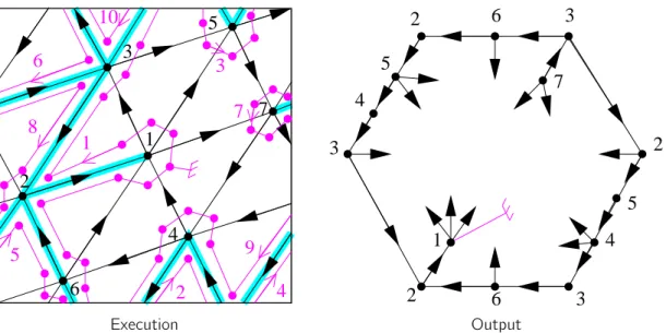
(12) Figure 1.6 – The minimal 3-orientation of the HTC-lattice of K7 w.r.t. the shaded face. Every oriented contractible cycle is counter-clockwise w.r.t. the shaded face.. Poulalhon et al.’s algorithm on oriented surfaces Here we introduce a reformulation of Poulalhon et al.’s original algorithm [85]. In an embedded graph G, a stem is an embedded arc whose origin is a vertex of G while its other end is not considered as a vertex. Algorithm PS Input : An oriented map G on an oriented surface S, a root vertex v0 and a root edge e0 incident to v0 . Output : A graph U with stems, embedded on S. The algorithm explores some of the edges of the map, marking one edge at each iteration. 1. Let v := v0 , e := e0 , U := ∅, Let all the edges being unmarked. 2. Let v 0 be the extremity of e different from v . Case 1 : e is non-marked and entering v . Add e to U and let v := v 0 . Case 2 : e is non-marked and leaving v . Add a stem to U incident to v and corresponding to e. Case 3 : e is already marked and entering v . Do nothing. Case 4 : e is already marked and leaving v . Let v := v 0 . 3. Mark e. 4. Let e be the next edge around v in counterclockwise order after the current e. 5. While (v , e) 6= (v0 , e0 ) go back to 2. 6. Return U. Let us stress the fact that the output of Algorithm PS is a graph embedded on the same surface as the input map but that this embedded graph is not necessarily a map (i.e some faces may not be homeomorphic to open disks). However, we showed that in a specific case the output U is an unicellular map, which is not the case for any input. We associate each couple (v , e) where e is incident to v , to the angle at v that is just before e in counterclockwise order. We thus call angle such couple. The particular choice of v0 and e0 thus defines a root face f0 : the face containing the angle (v0 , e0 ), that is the face just before e0 going around v0 counter-clockwisely. Figure 1.7 illustrates an execution of Algorithm PS . The condition in the while loop ensures that when the algorithm terminates, if it does, the algorithm is back to the root angle. The following proposition shows that the algorithm actually always terminates : 11.

(13) 10 3. 6. 1. 3. 5. 3. 7 4. 7 7. 8. 6. 2. 5. 1. 2. 3. 2 5 4 5 6. 2. 1. 9 4. 2. Execution. 4 6. 3. Output. Figure 1.7 – An execution of Algorithm PS on K7 given with the orientation corresponding to the minimal HTC 3-orientation of Figure 1.6. Vertices are numbered in black. The root angle, (1, 17), is identified by a root symbol and chosen in the face for which the orientation is minimal (i.e. the shaded face of Figure 1.6). The magenta points correspond to the angles considered at each iteration of Algorithm PS and the magenta arrows show the order in which those are considered. The output U is a toroidal unicellular map, represented here in an hexagon where the opposite sides are identified. Proposition 1.12. For every oriented map G on any oriented surface S and for any root angle (v0 , e0 ), the execution of Algorithm PS on (G, (v0 , e0 )) terminates. From toroidal triangulations to unicellular maps In the case of toroidal triangulations we know more on the behavior of Algorithm PS (See Figure 1.7). Theorem 1.13. Consider a toroidal triangulation T , a root angle (v0 , e0 ) such that v0 is not inside any separating triangle 7 , and the orientation of the edges of T corresponding to the minimal HTC 3-orientation w.r.t. the root face f0 . In this case, the output U of Algorithm PS is a toroidal spanning unicellular map, with the following properties : — Vertex v0 has three stems and the other vertices have two stems, but these values decrease by two for a vertex v if it is contained in two edge-disjoint cycles of U, or by one for a vertex v if it is contained in three (not necessarily edge-disjoint) cycles of U. — While walking along the unique face of U counter-clockwisely (according to this face) and starting at the root angle, at any moment, we have been along more edge sides (each edge of U has two sides on this boundary) than the number of stems we have met. — The orientation of U induced by the minimal HTC 3-orientation of T verifies the γ0 property (considering the edges and the stems of U). Note that every toroidal triangulation T has vertices that are not inside any separating triangles. Let us explain why this condition is necessary. In a 3-orientation of a toroidal triangulation, by Euler’s formula, all the edges that are incident to a separating triangle ∆ and in its interior are oriented towards the triangle. Thus if one applies Algorithm PS from a vertex inside ∆, the algorithm will remain in the interior of ∆, that is it will only consider angles (v , e) such that v is inside ∆. In this case the output cannot be spanning. 7. In other words, v0 does not belong to an open pseudo-disk of the torus whose boundary is a cycle of length three.. 12.

(14) Recovering the original triangulation Let us now show how to recover the original triangulation from the output of Algorithm PS. The method is very similar to [85] since like in the plane the output has only one face that is homeomorphic to an open disk. Theorem 1.14. Consider a toroidal triangulation T , a root angle (v0 , e0 ) such that v0 is not inside any separating triangle and the orientation of the edges of T corresponding to the minimal HTC 3-orientation w.r.t. the root face f0 . From the output U of Algorithm PS applied on (T, (v0 , e0 )) one can reattach all the stems to obtain T by starting at the root angle and walking along the face of U in counterclockwise order (according to this face) : each time a stem is met, it is reattached in order to create a triangular face on its left side. Figure 1.8 illustrates Theorem 1.14 on the example of Figure 1.7.. 6. 2. 3. 6. 2. 5. 3. 5 7. 7. 4. 4 2. 3. 2. 3. 5 1 2. 5. 4 6 First step. 1 2. 3 6. 2. 4 6 Second step. 3. 3. 5 7 4 2. 3 5 1 2. 4 6 Final step. 3. Figure 1.8 – How to recover the original toroidal triangulation from the output of Algorithm PS .. Bijections Actually the properties of U in Theorem 1.13 almost describe the outputs of Algorithm PS . Theorem 1.15. There is a bijection between n-vertex toroidal triangulations rooted at an angle (v0 , e0 ) such that v0 and e0 are not inside any separating triangle, and n-vertex unicellular maps verifying the properties of Theorem 1.13 and such that their root edge e0 is a stem 8 . 8. This comes from the fact that e0 is always outgoing v0 in the minimal HTC 3-orientation.. 13.

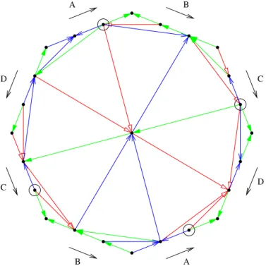
(15) Surprisingly, taking the outputs of Algorithm PS , removing their root stem and forgetting the orientation of their edges one obtains an interesting familly of unrooted unicellular maps. We obtained the following bijection on unrooted toroidal maps. Theorem 1.16. There is a bijection between the set of n-vertex toroidal maps, where all the faces have length three, except one that has length four and which is not inside a separating triangle, and the set of n-vertex toroidal unicellular maps, with the following properties : — Every vertex has two stems, but this value decreases by two for a vertex v if it is contained in two edge-disjoint cycles, or by one for a vertex v if it is contained in three (not necessarily edge-disjoint) cycles. — Considering only the stems, the map verifies the γ0 property. These unicellular maps are rather simple, and Theorem 1.16 can thus be used to compute the number of such n-vertex quasi-triangulations 9 , and maybe also to sample them. The only difficulty comparing to the planar case is the γ0 property. Conclusion Note that Algorithm PS has been studied by other researchers [5, 11], in particular for maps embedded on genus g ≥ 1 surfaces. Contrarily to [11] our maps T and U have the same genus. This is interesting as fixed genus unicellular maps are getting better understood [29]. The key property that makes U and T have same genus is that there is no non-contractible curve C of the torus such that all the arcs of T crossing C cross it in the same direction. We proved [J22] that any simple triangulation of a genus g ≥ 1 orientable surface admits an orientation of its edges such that every vertex has outdegree at least 3, and divisible by 3. The following would ensure use that Algorithm PS behaves well (i.e. produces a spanning unicellular map). Conjecture 1.17. A triangulation on a genus g ≥ 1 orientable surface admits an orientation of its edges such that every vertex has outdegree at least 3, divisible by 3, and such that there is no non-contractible curve C of the torus such that all the arcs crossing C cross it in the same direction. If Conjecture 1.17 is true, one can consider a minimal orientation satisfying its conclusion 10 and apply Algorithm PS to obtain a unicellular map of the same genus. Note that more efforts should be made to obtain a bijection since there might be several minimal orientations 11 satisfying the conjecture and a particular one has to be identified (as the minimal HTC 3-orientation in our case).. 1.4. Extensions to (oriented) Surfaces with higher Genus. For higher genus triangulated surfaces, a generalization of Schnyder woods has been proposed by Castelli Aleardi et al. [21], with applications to encoding. In this definition, the simplicity and the symmetry of the original definition of Schnyder woods are lost. Here we propose an alternative generalization of Schnyder woods for higher genus that generalizes the one proposed in [J18] for the toroidal case. We consider finite maps. Denote by n, m and f the number of vertices, the number of edges, and the number of faces of a map. Euler’s formula says that any map on an orientable surface of genus g satisfies n − m + f = 2 − 2g. This implies that a triangulation of genus g has exactly 3n + 6(g − 1) edges. So to generalize Schnyder woods for all g ≥ 2 there are too many edges to force all vertices to have outdegree exactly three. This problem can be overcome by allowing vertices to fulfill the Schnyder property (cf Definition 1.1) “several times”, i.e. such vertices have outdegree 6, 9, etc. with the color property of Figure 1.1.(a) repeated several times (see Figure 1.9). ´ Fusy and B. L´ 9. This was not included in [J24] but should appear in a paper by E. evˆ eque. 10. Note that reversing contractible directed cycles preserves the properties of Conjecture 1.17. 11. Each of these orientations being the unique minimal element in their lattice.. 14.

(16) Outdegree six. Outdegree nine. Figure 1.9 – The Schnyder property repeated several times around a vertex.. Figure 1.10 is an example of such a Schnyder wood on a triangulation of the double torus. The double torus is represented by in an octagon whose sides are pairwisely identified as indicated. All the vertices of the triangulation have outdegree three except two vertices, the circled ones, that have outdegree six. Each of the latter appear twice in the representation. A. B. D. C. D. C. B. A. Figure 1.10 – A Schnyder wood of a triangulation of the double torus. We formalized in [S2] a concept of weak Schnyder woods 12 for general maps (not only triangulations) on arbitrary orientable surfaces. These are defined via angle labelings in Section 1.4.1. Then in Section 1.4.2, we characterize the orientations that correspond to these weak Schnyder woods. While every map admits a “trivial” Schnyder wood, the existence of a non-trivial one remains open but leads to interesting conjectures. 12. We call them weak Schnyder woods in this manuscript because for the torus the definition will be weaker than Definition 1.5.. 15.

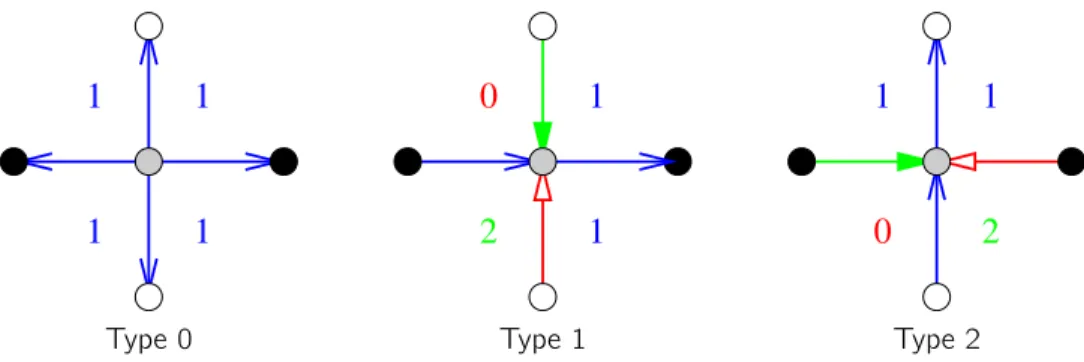
(17) 1.4.1. Angle labelings. Consider a map G on an orientable surface. An angle is a face corner at a vertex, and an angle labeling of G is a labeling of its angles with colors 0, 1, 2. More formally, we denote an angle labeling by a function ` : A → Z3 , where A is the set of angles of G. Given an angle labeling, we define several properties of vertices, faces and edges that generalize the notion of Schnyder angle labeling in the planar case [47]. Consider an angle labeling ` of G. A vertex or a face v is of type k, for k ≥ 1, if the labels of the angles around v form, in counterclockwise order, 3k nonempty intervals such that in the j-th interval all the angles have color (j mod 3). A vertex or a face v is of type 0, if the labels of the angles around v are all of color i for some i in {0, 1, 2}. An edge e is of type 1 or 2 if the labels of the four angles incident to this edge are, in clockwise order, i − 1, i , i , i + 1 for some i in {0, 1, 2}. The edge e is of type 1 if the two angles with the same color are incident to the same extremity of e and of type 2 if the two angles are incident to the same side of e. An edge e is of type 0 if the labels of the four angles incident to e are all i for some i in {0, 1, 2} (See Figure 1.11). If every vertex (resp. edge, or face) x of G is of type f (x), for some function f : X → N, we say that ` is VERTEX (resp. EDGE, or FACE). If every vertex (resp. edge, or face) x of G is of type 1, we say that ` is 1-VERTEX (resp. 1-EDGE, or 1-FACE). If every vertex (resp. face) x of G is of type f (x), for some function f : X → N∗ = N \ {0}, we say that ` is N∗ -VERTEX (resp. N∗ -FACE). The following lemma expresses that property EDGE is the central notion here. Lemma 1.18. Any EDGE angle labeling is VERTEX and FACE. Thus we define weak Schnyder labeling and weak Schnyder woods as follows : Definition 1.19 (weak Schnyder labeling). Given a map G on an orientable surface, a weak Schnyder labeling of G is an EDGE angle labeling of G. A weak Schnyder wood is an orientation and coloring of the edges of G with edges oriented in one direction or in two opposite directions if it is obtained by applying the rules of Figure 1.11 from a weak Schnyder labeling of G.. 1 1 Type 0. 1. 0. 1. 2 Type 1. 1. 1. 1. 0. 1 2 Type 2. Figure 1.11 – Correspondence between EDGE angle labelings and some bi-orientations and colorings of the edges. Any map (on any orientable surface) admits a trivial EDGE angle labeling : the one with all angles labeled i (and thus all edges, vertices, and faces are of type 0). A natural non-trivial case, that is also symmetric for the duality, is to consider EDGE, N∗ -VERTEX, N∗ -FACE angle labelings of general maps. In planar Schnyder woods only type 1 and type 2 edges are used. Here we allow type 0 edges because they seem unavoidable for some maps (see discussion below). Figure 1.10 is an example of a weak Schnyder wood obtained from an EDGE, N∗ -VERTEX, N∗ -FACE angle labelings. For every g ≥ 2, there are genus g maps, with vertex degrees and face degrees at most five. Figure 1.12 depicts how to construct such maps, for all g ≥ 2. For these maps, type 0 edges are unavoidable. Indeed, take such a map with an angle labeling that has only type 1 and type 2 edges. Around a type 1 or type 2 edge there are exactly three changes of labels, so in total there are exactly 3m such changes. As vertices and faces have degree at most five, they are either of type 0 or 1, hence the number of label changes should be at most 3n +3f . Thus, 3m ≤ 3n + 3f , which contradicts Euler’s formula for g ≥ 2. Furthermore, note that the maps described in Figure 1.12, as well as their dual maps, are 3-connected. Actually they can be modified to be 4-connected 16.

(18) and of arbitrary large face-width 13 . Note that these maps admit EDGE, N∗ -VERTEX, N∗ -FACE angle labelings (using type 0 edges), but those are not described in this manuscript.. Gi. f’i. f’i. fi. fi. Figure 1.12 – A toroidal map Gi with two distinguished faces, fi and fi 0 . Take g copies Gi with 1 ≤ i ≤ g and 0 glue them by identifying fi and fi+1 for all 1 ≤ i < g. Faces f1 and fg0 are filled to have only vertices and faces of degree at most five. The planar maps that admit a planar Schnyder wood ar exactly the internally 3-connected ones (c.f. Theorem 1.4). We similarly showed that a toroidal map admits a Schnyder wood, if and only if it is essentially 3-connected (c.f. Theorem 1.8). We showed the following for weak Schnyder labelings. Theorem 1.20. If a map G on a genus g ≥ 1 orientable surface admits an EDGE, N∗ -VERTEX, N∗ -FACE angle labeling, then G is essentially 3-connected. We conjecture that this characterizes the maps that admit such angle labelings. Conjecture 1.21. A map on a genus g ≥ 1 orientable surface admits an EDGE, N∗ -VERTEX, N∗ -FACE angle labeling if and only if it is essentially 3-connected. As we will see in Section 1.5, and as already mentioned, every simple triangulation on a genus g ≥ 1 orientable surface admits an orientation of its edges such that every vertex has outdegree at least three, and divisible by three. This suggests the existence of 1-EDGE angle labelings with no sinks, i.e. 1-EDGE, N∗ -VERTEX angle labelings. One can easily check that in a triangulation, a 1-EDGE angle labeling is also 1-FACE. Thus we can hope that a triangulation on a genus g ≥ 1 orientable surface admits a 1-EDGE, N∗ -VERTEX, 1-FACE angle labeling. Note that a 1-EDGE, 1-FACE angle labeling of a map implies that faces have size three. So we propose the following conjecture, whose “only if” part follows from the previous sentence : Conjecture 1.22. A map on a genus g ≥ 1 orientable surface admits a 1-EDGE, N∗ -VERTEX, 1-FACE angle labeling if and only if it is a triangulation. Conjecture 1.21 implies Conjecture 1.22 since for a triangulation every face would be of type 1, and thus every edge would be of type 1. Conjecture 1.21 is proved for g = 1 [J18] whereas both conjectures are open for g ≥ 2. 13. For many problems, maps with high face-width are easier to handle. The face-width of a map G is the smallest number k such that there is a non-contractible closed curve that intersects G in k points.. 17.

(19) 1.4.2. Orientations of weak Schnyder woods. It was shown by de Fraysseix et al. [58], that for any planar triangulation every orientation of its inner edges where every inner vertex has outdegree three corresponds to a Schnyder wood. Thus, any orientation with the proper outdegree corresponds to a Schnyder wood and there is a unique way, up to symmetry of the colors, to assign colors to the oriented edges in order to fulfill the Schnyder property at every inner vertex. This is not true in higher genus as already in the torus, there exist orientations that do not correspond to any Schnyder wood (see Figure 1.13), not even to a weak Schnyder wood.. Figure 1.13 – Two different orientations of a toroidal triangulation. Only the one on the right corresponds to a (weak) Schnyder wood. Consider a map G on an orientable surface of genus g. The orientation of G defined by a weak Schnyder woods can be defined more naturally in the primal-dual-completion of G, as there is no more edges oriented in two directions. The primal-dual-completion Gˆ is the map obtained from simultaneously embedding G and G ∗ such that vertices of G ∗ are embedded inside faces of G and vice-versa. Moreover, each edge crosses its dual ˆ Hence, Gˆ is a bipartite graph with one edge in exactly one point in its interior, which also becomes a vertex of G. part consisting of primal-vertices and dual-vertices and the other part consisting of edge-vertices (of degree four). Each face of Gˆ is a quadrangle incident to one primal-vertex, one dual-vertex and two edge-vertices. Actually, the faces of Gˆ are in correspondance with the angles of G. This means that angle labelings of G ˆ correspond to face labelings of G. Given α : V → N, an orientation of G is an α-orientation [46] if for every vertex v ∈ V its outdegree d + (v ) equals α(v ). We call an orientation of Gˆ a mod 3 -orientation if it is an α-orientation for a function α satisfying : ( 0 (mod3) if v is a primal- or dual-vertex, α(v ) ≡ 1 (mod3) if v is an edge-vertex. Note that an EDGE angle labeling (i.e. a weak Schnyder wood) of G corresponds to a mod3 -orientation ˆ by the mapping of Figure 1.14, where the three types of edges are represented. Type 0 corresponds of G, to an edge-vertex of outdegree four. Type 1 and type 2 both correspond to an edge-vertex of outdegree 1 ; in type 1 (resp. type 2) the outgoing edge goes to a primal-vertex (resp. dual-vertex). In all cases we have d + (v ) ≡ 1 (mod3) if v is an edge-vertex. By Lemma 1.18, the labeling is also VERTEX and FACE. Thus, d + (v ) ≡ 0 (mod3) if v is a primal- or dual-vertex. As mentioned earlier, de Fraysseix et al. [58] showed for planar triangulations, that every internal 3orientations corresponds to a Schnyder wood. Felsner [46] generalized this result for planar Schnyder woods and orientations of the primal-dual completion having prescribed out-degrees. The situation is more complicated in higher genus (see Figure 1.13). It is not enough to prescribe outdegrees in order to characterize orientations corresponding to weak Schnyder woods. We call an orientation of Gˆ corresponding to a weak Schnyder wood of G a weak Schnyder orientation. In the following we show how to characterize these orientations. Consider a (not necessarily directed) cycle C of G together with a direction of traversal. We associate to C ˆ We define γ(C) by : its corresponding cycle in Gˆ denoted by C. γ(C) = # edges of Gˆ leaving Cˆ on its right − # edges of Gˆ leaving Cˆ on its left. 18.

(20) 1. 1. 0. 1. 1. 1. 1. 1. 2. 1. 0. 2. Type 0. Type 1. Type 2. Figure 1.14 – How to map a weak Schnyder labeling to a mod3 -orientation of the primal-dual completion. Primal-vertices are black, dual-vertices are white and edge-vertices are gray. Theorem 1.23. Consider a map G on an orientable surface of genus g. Let {B1 , . . . , B2g } be a set of cycles of G that forms a basis for the homology. An orientation of Gˆ is a weak Schnyder orientation if and only if it is a mod 3 -orientation such that γ(Bi ) ≡ 0 (mod3), for all 1 ≤ i ≤ 2g. For a given map G, the set of weak Schnyder orientations of Gˆ with same values γ(B1 ), . . . , γ(B2g ) has a ˆ are linked if they differ only on a directed closed walk W that lattice structure. The elements (orientations of G) is null-homologous. If W is a directed separating cycle (which is thus null-homologous), it crosses Bi from left to right as many times as it crosses it from right to left. It is thus clear (in this case) that reversing the edges of W does not change γ(Bi ). In Section 1.3.2 we used the fact that for toroidal triangulations, all the orientations of Gˆ corresponding to (non-weak) Schnyder woods belong to the same lattice. This lattice is the one for which γ(Bi ) = 0, for all 1 ≤ i ≤ 2g. Note that this does not depend on the choice of the basis {B1 , . . . , B2g } as in this case γ(C) = 0 for every non-contractible cycle C.. 1.5. (0 mod 3)-Orientations. This section is devoted to the following theorem [J22] that was conjectured by Bar´ at et al. [9]. Theorem 1.24. Every simple triangulation T of a surface of Euler genus 14 k ≥ 2 has an orientation such that each outdegree is at least 3, and divisible by 3. Bar´ at et al.’s proved it for small Euler genus, and for any Euler genus, they proved a weaker version where sinks (i.e. outdegree zero vertices) are allowed. Their conjecture was originally motivated in the context of claw-decompositions of graphs, since given an orientation with the claimed properties the outgoing edges of each vertex can be divided into claws, such that every vertex is the center of at least one claw. Our motivation was more related to Conjecture 1.22, as Theorem 1.24 may be a step towards proving this conjecture. Similarly, answering to the following conjecture would be a step towards Conjecture 1.21 . Conjecture 1.25. Given an essentially 3-connected map G, its primal-dual-completion Gˆ has an orientation where primal- and dual-vertices have non-zero outdegrees divisible by three, and where edge-vertices have indegrees divisible by three, that is indegree 0 or 3 (i.e. outdegree 4 or 1). Recall also that Conjecture 1.17 asks for an improvement of Theorem 1.24 towards obtaining orientations of triangulations that behave well with respect to Algorithm PS . Before going into the proof of Theorem 1.24 let us define induced submaps. Given a triangulation T and a set of vertices X ⊆ V (T ), the induced submap T [X] is simply the maximal submap with vertex set X. In other words this submap has edge set {uv ∈ E(T ) | u ∈ X and v ∈ X}, and face set {uv w ∈ F (T ) | u ∈ X, v ∈ X, and w ∈ X}. Note that submaps are thus embedded graphs with (a few) faces, that are a subset of the embedded graph’s faces. 14. The Euler genus of a map is 2 − n + m − f , where n, m and f stand for the number of vertices, edges, and faces.. 19.

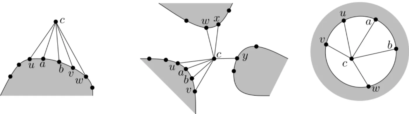
(21) 1.5.1. Proof of Theorem 1.24. We consider a triangulation T that is a minimal counter example. Then there are several stages. We first prove that one can partition the edges of the triangulation T into the following graphs : — The initial graph I, which is an induced submap containing a non-contractible cycle. Furthermore, I contains an edge uv such that the map I \ uv is a maximal outerplanar graph with only two degree two vertices, u and v . See Figure 1.15 for an illustration.. u v. Figure 1.15 – Example of a submap I.. — The correction graph B (with blue edges), which is oriented acyclically in such a way that each vertex of V (T ) \ V (I) has outdegree 2, while the other vertices have outdegree 0, — The last correction path G (with green edges), which is a {u, v }-path. — The non-zero graph R (with red edges), which is oriented in such a way that all vertices in (V (T ) \ V (G))∪ {u, v } have out-degree at least 1.. Finding the submap I We do not explain this not very interesting part of the proof. Constructing B, G, and R Starting from I we incrementally explore the whole triangulation T by stacking the vertices one by one (this procedure is inspired by [21]). At each step, we will assign the newly explored edges to B, G or R, and we will orient those assigned to B or R. At each step the explored region is a submap of T induced by some vertex set X. Such explored region is denoted by T [X] and its boundary ∂T [X] (See Figure 1.16 for an illustration).. 20.

(22) u. wx. c. a. v u a. c bv. w. ua b v. y. b c w. Figure 1.16 – Different types of stacking a vertex c on an induced submap M (grey region). Left : one neighboring path P1 = (u, a, b, v , w ). Middle : three neighboring paths P1 = (u, a, b, v ), P2 = (w , x), P3 = (y ). Right : A boundary cycle C = (u, v , w , b, a).. During the exploration we maintain the following invariants : (I) The graphs I, B, G, and R partition the edges of T [X]. (II) All interior vertices of T [X] (i.e. in X \ V (∂T [X])) have at least one outgoing R-arc, or two incident G-edges. Furthermore G either is an {u, v }-path, or is the union of two vertex disjoint paths Gu and Gv , going from u to u∗ , and from v to v∗ , respectively, for some vertices u∗ and v∗ on ∂T [X]. Here the vertices u∗ and v∗ may coincide with vertices u and v , respectively, if Gu or Gv is trivial. (III) The graph B is acyclically oriented in such a way that the vertices of I have outdegree 0, while the other vertices of T [X] have outdegree 2. Furthermore, to help us in properly finishing the construction of the graphs B, G and R in the further steps, we introduce the notion of requests on the angles 15 of ∂T [X]. There are two types of requests, G-requests and R-request. An angle is allowed to have at most one request, and an angle having no request is called free. Informally, a G-request (resp. an R-request) for an angle ab means that in a further step an edge inside this angle will be added in G (resp. in R and oriented from a to the other end). (IV) Every vertex of (∂T [X] \ {u∗ , v∗ }) ∪ {u, v } having (still) no outgoing R-arc, has an incident angle with an R-request.. (V) If G is not a {u, v }-path (yet), the vertices u∗ and v∗ (at the end of Gu and Gv , respectively), have one incident angle each, say c u∗ and c v∗ , that are consecutive on ∂T [X], and that have a G-request. Furthermore, there are no other G-requests. (VI) If there is an unexplored disk D 16 , then there are at least three free angles (of ∂T [X]) around D.. One can observe that if these invariants are maintained until the end of the exploration, we obtain the desired partition of the edges.. 15. Here an angle is a triplet (e, v , e 0 ) of consecutive elements of ∂T [X]. 16. An unexplored disk D is an open pseudo disk that does not intersect T [X] but whose border is contained in T [X].. 21.

(23) u v. Figure 1.17 – Assigning requests to I in order to satisfy the invariants. G-requests are green, R-requests are red.. The exploration starts with T [X] = I with the following setting of requests on the angles (see Figure 1.17). Set the angles of consecutive appearance of u, v as G-requests, while all the other angles are assigned Rrequests. Then one can check that (I)-(VI) are satisfied. We do not explain here how to choose the next vertex to stack, how to partition and color the new edges, nor how to assign requests to the new angles. Reorienting B Here we use the same approach as in the proof of Theorem 4.5 in [9]. Given a partial orientation O of T + + we define the demand of a vertex v as demO (v ) := −δ|O (v ) mod 3, where δ|O (v ) denotes the outdegree of v with respect to O. We want to find an orientation of T with all demands 0. We do not modify the orientation on R, and this guarantees that all vertices in (V (T ) \ V (G)) ∪ {u, v } have non-zero outdegrees. Furthermore, as G will be oriented either entirely forward or backwards (this will be chosen later), all its interior vertices will have non-zero outdegrees. Hence every vertex of T [X] has non-zero outdegree. Suppose that G is entirely oriented forward. Now we linearly order vertices in V (T ) \ V (I) = (v1 , . . . , v` ) such that with respect to B every vertex has its two outgoing B-neighbors among its predecessors and I (this corresponds to the order the stacking was performed). Denote by Bi the subgraph of B induced by the arcs leaving vi , . . . , v` (before the reorienting). We process V (T ) \ V (I) from the last to the first element. At a given vertex vi we look at demG∪R∪Bi (vi ) and reorient the two originally outgoing B-arcs of vi in such a way that afterwards demG∪R∪Bi (vi ) = 0 (i.e. + δ|G∪R∪B (vi ) ≡ 0 mod 3). As these B-arcs were heading at I or at a predecessor, the demand on the vertices i vj , with j > i , is not modified and hence remains 0. Denote by O the obtained partial orientation of T . Orienting G and I Now pick an orientation of G (either all forward or all backward) and of uv such that for the resulting partial orientation O0 we have demO0 (v ) = 1. Let ∆ be the triangle of I containing v . Since I \ uv is a maximal outerplanar graph it can be peeled by removing degree two vertices until reaching ∆. When a vertex x is removed orient its two incident edges so that demO0 (x) = 0 (as for B-arcs). We obtain a partial orientation O00 , such that 22.

(24) all vertices have non-zero outdegree, and such that all vertices except the ones of ∆ have outdegree divisible by 3. Since the number of edges of T , and the number of edges of ∆ are divisible by 3, the number of edges of T \ ∆ is divisible by 3. As this number equals the sum of the outdegrees in O00 , and as every vertex out of ∆ has outdegree divisible by 3, then the outdegree of ∆’s vertices sum up to a multiple of 3. Hence their demands sum up to 0, 3 or 6. As demO00 (v ) = demO0 (v ) = 1, the demands of the other two vertices of ∆ are either both 1, or 0 and 2. It is easy to see that in either case ∆ can be oriented to satisfy all three demands.. 23.

(25) 24.

(26) Chapitre 2. Intersection Representations for Planar Graphs 2.1. Introduction. Intersection graphs form a large part of nowadays studied classes of graphs. This chapter will only cover a small part of this broad research area. We will only consider intersection graphs of connected shapes in the plane. Research on representations of (planar) graphs by contact or intersection of predefined shapes in the plane started with the work of Koebe in 1936 [71]. Given a shape 1 X, an X-intersection representation is a collection of X-shaped geometrical objects in the plane. The X-intersection graph described by such a representation has one vertex per geometrical object, and two vertices are adjacent if and only if the corresponding objects intersect. An intersection representation of a graph G = (V, E) is thus an intersection representation C = {c(v ) : v ∈ V }, such that two geometrical objects, c(u) and c(v ), intersect if and only if their corresponding vertices are adjacent, i.e. uv ∈ E. The shapes that are homeomorphic to a segment or to a disk are respectively referred to as pseudo-segments or as pseudo-disks. If the shape X is a pseudo-segment (resp. a pseudo-disk), an X-contact representation is an X-intersection representation such that if an intersection occurs between two objects, then it occurs at a single point that is the endpoint of one of them (resp. it occurs on their boundary). We say that a graph G is an X-contact graph if it is the X-intersection graph of an X-contact representation.. 2.1.1. Pseudo-disks. The case of shapes homeomorphic to discs has been widely studied ; see for example the literature for disks [71, 6, 33], triangles [57, J13], homothetic triangles [69, 92], rectangles [97, 54], squares [91, 74], hexagons [63], convex bodies [90], or (non-convex) axis aligned polygons [4]. Most of these works actually deal with contact representations. A contact point of a contact representation is a point that is in the intersection of (at least) two shapes. A contact representation is said simple if for any two intersecting shapes there is a contact point contained by these two shapes only. Observe that a simple contact representation by pseudo-disks C = {c(v ) : v ∈ V } necessarily represents a plane graph. Indeed, one can draw the represented graph by choosing any point pv inside c(v ), for representing each vertex v , and by drawing curves from pv to the “private” contact points around c(v ) to represent the edges incident to v . The circle packing theorem of Koebe [71] states that every planar graph admits a contact representation by circles. Here, vertices are represented by homothetic objects, circles. Another case has been explored, the case 1. We do not provide a formal definition of shape, but a shape characterizes a family of connected geometric objects in the plane.. 25.

(27) of squares, using different tools [91, 74]. Both papers show that 5-connected planar triangulations minus one edge are contact graphs of axis parallel squares. Several works considered contact representations by shapes that are not necessarily homothetic. Koebe’s theorem implies that every planar graph has a contact representation by convex polygons, and de Fraysseix et al. [57] strengthened this by showing that every planar graph admits a contact representation by triangles. Thomassen [97] considered the contact graphs of axis parallel rectangles. One can observe that such contact representation provides (following the procedure described above) a plane graph where each triangle bounds an inner face. Thomassen proved that this property characterizes these contact graphs. In other words these contact graphs are exactly the proper subgraphs (i.e. strict subgraphs) of 4-connected planar triangulations. The subgraphs being proper one can draw them so that the outerface has length at least four, and the 4connectedness ensures that every triangle bounds an inner face. Fusy [61, 62] then studied the structures (named transversal structures) defined by such contact representations, and used those to design new bijections (linking triangulations and loopless maps) and a drawing algorithm. Gansner et al. [63] proved that every planar graph has a contact representation with convex hexagons which sides use only 3 slopes (i.e. hexagons with two horizontal sides and which angles are all 32 π) and where the intersection between two shapes is a segment (not a single point). Using non-combinatorial arguments Schramm proved a powerfull and very general result, sometimes referred to as the monster packing theorem. This theorem deals with any kind of convex shapes [90]. Theorem 2.1 (monster packing theorem [90]). Let T be a planar triangulation with outerface abc. Let C be a simple closed curve in the plane, and let c(a), c(b), c(c) be three arcs composing C, which are determined by three distinct points of C. For each vertex v ∈ V (T ) \ {a, b, c}, let there be a prototype Pv , which is a convex shape in the plane containing more than one point. Then there is a contact representation in the plane C = {c(v ) : v ∈ V (T )}, where each c(v ) for v ∈ V (T ) \ {a, b, c} is either degenerated to a point or (positively) homothetic to Pv , and such that T is a subgraph of the contact graph induced by C. We will see in Section 2.2 how this led us to prove the following theorem that was conjectured by Kratochv´ıl [73] (see also [8]). Theorem 2.2. Every 4-connected planar triangulation admits a contact representation by homothetic triangles. Then we will use this result as a building block for proving the following result. Theorem 2.3. A graph is planar if and only if it is the intersection graph of homothetic triangles, where the intersection of any three triangles is empty. This answers a conjecture of Lehmann that planar graphs are max-tolerance graphs (as max-tolerance graphs have shown to be exactly the intersection graphs of homothetic triangles [69]). There are also many works dealing with contact representations by non-convex shapes such as axis aligned polygons. In order to bypass the limitations of rectangular cartograms [96], researcher studied cartograms for visualization purposes (e.g. for geographical data) [4]. These cartograms are actually contact representations by polygons which sides are axis parallel. From Thomassen’s characterization of contact representations by rectangles, it follows that every 4-connected triangulation admits a contact representation by L-shaped hexagons. We improved this a bit by restraining ourselves to L-shaped hexagons drawn on the integer grid so that the branches of each L are one unit thick (i.e. the topmost and rightmost sides have length one), and so that two touching L’s touch on a segment 2 . We call such a representation a thick L contact representation. Theorem 2.4. Every 4-connected triangulation admits a thick L contact representation. We will sketch the proof of this result in Section 2.5.2. 2. This deviate’s a little from the original result in [C25] where L’s can intersect on a single point.. 26.

(28) A primal-dual contact representation (V, F) of a planar map G is a pair of contact representations V = {c(v ) : v ∈ V (G)} and F = {c(f ) : f ∈ V (G ∗ )}, such that V is a contact representation of G, and F is a contact representation of G ∗ , the dual of G, and for every edge uv , bordering faces f and g, the intersection between c(u) and c(v ) equals the intersection between c(f ) and c(g). Andre’ev [6] strengthened Koebe’s theorem as follows : Theorem 2.5 (Andre’ev [6]). Every 3-connected planar map admits a primal-dual contact representation by circles. We proved an analogous result concerning contact representations by triangles. We say that a primal-dual contact representation by triangles is tiling if the triangles corresponding to vertices and those corresponding to inner faces form a tiling of the triangle corresponding to the outer face (see Figure 2.1).. Figure 2.1 – A tiling primal-dual contact representation by triangles. Theorem 2.6. Every internally 3-connected planar map admits a tiling primal-dual contact representation by triangles. In [64], Gansner et al. study representation of graphs by triangles where two vertices are adjacent if and only if their corresponding triangles are intersecting on a segment (they call them touching representation by triangles). Theorem 2.6 shows that for 3-connected planar graphs, the incidence graph between vertices and faces admits a touching representation by triangles. We will sketch the proof of Theorem 2.6 in Section 2.3.. 2.1.2. Pseudo-segments. In his PhD thesis [87], Scheinerman conjectured that every planar graph has an intersection representation by segments. Several results partially confirmed this conjecture. Hartman et al. [66], de Fraysseix et al. [41], and Czyzowicz et al. [34] proved it for bipartite planar graphs. The case of triangle-free planar graphs was proved by de Castro et al. [23] and more recently de Fraysseix et al. [43] proved it for every planar graph that has a 4-coloring in which every induced cycle of length 4 uses at most 3 colors. We provided two proofs of this conjecture [C12, C25], the most recent one being much simpler that the former one. In this manuscript we will 27.

(29) sketch both proofs (in Section 2.4.3 and in Section 2.5), and we will explain intermediate results that led us to these proofs. To explain these intermediate results, we need a few definitions. Here, we focus on intersection and contact representations of planar graphs with different types of pseudosegments. The more general representations of this type are the intersection or contact representations with pseudo-segments (also known as strings in this context). It is known that every planar graph has an intersection representation by strings [38]. Indeed, one just has to take a contact representation by circles, and cut the circles to turn them into strings. If one wants to avoid tangent points it suffices to inflate the circles a little. In this case, a pair of strings can cross each other at most twice. Definition 2.7. A 1-string representation of a graph is an intersection representation by strings where (1) strings cannot intersect tangentially, and where (2) every two strings intersect at most once. Seeking a proof of Scheinerman’s conjecture, it was suggested [42, 72] to first prove it for slack segments, with the idea in a second time to stretch them and obtain a segment representation. Thus condition (1) and (2) of Definition 2.7 are necessary. This approach of Scheinerman’s conjecture was decisive since we first proved that every planar graph has a 1-string representation [J9], and then we manage to improve this proof to obtain the first proof of Scheinerman’s conjecture [C12]. Theorem 2.8. Every planar graph has a 1-string representation. Theorem 2.9. Every planar graph has a segment intersection representation. However, note that the latter construction is not a stretching of the former one. One difficulty in these constructions is that the obtained representations somehow violate the original embedding of the planar graph. Actually, Biedl et al. [15] showed that some planar graphs, like planar 3-trees, do not have an order-preserving 1-string representation (that is a representation where the order of the crossings allong a string follow the order of the edges around the corresponding vertex). In order to introduce the second proof of Scheinerman’s conjecture we need to define the following graph classes. A graph is said to be a VPG-graph (Vertex-Path-Grid) if it has a contact or intersection representation in which each vertex is assigned to a path of vertical and horizontal segments (see [2, 32]). Asinowski et al. [7] showed that the class of VPG-graphs is equivalent to the class of graphs admitting a string representation. They also defined the class Bk -VPG, which contains all VPG-graphs for which each vertex is represented by a path with at most k bends (see [55] for the determination of the value of k for some classes of graphs). It is known that Bk -VPG ( Bk+1 -VPG, and that the recognition of graphs of Bk -VPG is an NP-complete problem [26]. These classes have interesting algorithmic properties (see [77] for approximation algorithms for independence and domination problems in B1 -VPG graphs), but most of the literature studies their combinatorial properties. Chaplick et al. [28] proved that planar graphs are B2 -VPG graphs. This result was recently improved by Biedl et al. [13], as they showed that planar graphs have a 1-string B2 -VPG representation. Various classes of graphs have been shown to have 1-string B1 -VPG representations, such as planar partial 3-trees [12] and Halin graphs [40]. In these representations, each vertex is assigned to a path formed by at most one horizontal and one vertical segment. There are different types of such paths. For example, the x shape defines paths where the vertical segment is above and to the left of the horizontal one. Interestingly, it has been shown that the class of simple segment contact graphs is equivalent to the one of B1 -VPG contact graphs [70]. This implies in particular that triangle-free planar graphs are B1 -VPG contact graphs. This has been improved by Chaplick et al. [28] as they showed that triangle-free planar graphs are in fact {x, p, |, −}-contact graphs (that is without using the shapes y and q). In the following, we will always precise when | or − shapes are allowed. This is particularly important as for example some {x, |, −}-contact graphs, like the triangular prism, are not x-contact graphs. The restriction of B1 -VPG to x-intersection or x-contact graphs has been much studied (see for example [55]) and it has been shown that they are in relation with other structures such as Schnyder realizers, canonical orders or edge labelings [27]. The same authors also proved that the recognition of x-contact graphs can be done 28.

(30) in quadratic time, and that this class is equivalent to the one restricted to equilateral x shapes. The x-contact graphs where the corners lie on a straight line are called monotone or linear x-contact graphs. Those graphs have been recently studied further, in particular in relation with MPT (Max-Point Tolerance) graphs [24, 3]. In section 2.5 we will prove the following theorems that were both conjectured by Chaplick et al. [28] 3 . Theorem 2.10. Every triangle-free planar graph has a (simple) {x, |, −}-contact representation. Theorem 2.11. Every planar graph has an x-intersection representation. In both cases, one cannot restrict the representation to | and − shaped paths. Indeed, any {|, −}-intersection representation of a triangle-free planar graph defines a vertex partition of the graph into two forests of paths (one induced by the vertical paths and the other induced by the horizontal ones), but such partition is not always possible [93]. As a contact graph of a simple string representation with n vertices has at most 2n edges and as a trianglefree planar graph may have up to 2n − 4 edges, Theorem 2.10 cannot be extended to much denser graphs. However, for planar Laman graphs (a large family of planar graphs with at most 2n − 3 edges and which are B1 -VPG intersection graphs [55]), the question of whether these graphs have a {x, |, −}-contact representation is open, up to our knowledge. The question whether triangle-free planar graphs are {x, |}-contact graphs is also open. Theorem 2.11 implies that planar graphs are 1-string B1 -VPG, improving the results of Biedl and Derka [13] stating that planar graphs are 1-string B2 -VPG. Since an {x, p, |, −}-intersection representation can be turned into a segment intersection representation [78], Theorem 2.11 provides a rather simple proof of Scheinerman’s conjecture.. 2.2. Representations by Homothetic Triangles. Theorem 2.1 is the building block for the results presented in this section. As already observed, simple contact representations produce planar graphs, so by ensuring that the representation C produced by Theorem 2.1, from a triangulation T , is (almost) simple we obtain that the contact graph of C is actually T itself (by maximality of planar triangulations). We ensure this “almost simplicity” of C by adding a natural condition on the prototypes : In a contact representation by pseudo-disks, one can draw the induced graph by choosing an arbitrary point in each set and drawing the edges uv between the corresponding points, inside the region c(u) ∪ c(v ) and hence passing through a contact point of c(u) and c(v ). With such a drawing one can see that the graph induced by the contact representation is a planar graph where some faces are turned into complete graphs (such a complete graph on k ≥ 4 vertices corresponds to k shapes intersecting at a given point). With such a complete graph on k ≥ 4 vertices, the contact graph is generally non-planar. We are hence going to forbid k intersecting shapes for k ≥ 4, and even for k = 3 in some cases. Theorem 2.12. Consider a k-connected triangulation T , for k ∈ {3, 4, 5}, and a set of prototypes {Pv : v ∈ V (T )}, that are convex and with more than one point. If every non-facial cycle (v1 , . . . , vl ), with l ≥ k is such that homothets of Pv1 , . . . , Pvl cannot intersect at a single point, then T has a planar contact representation C = {c(v ) : v ∈ V (T )}, where each c(v ) is a positive homothet of Pv . Note that one cannot drop the 4-connectedness (to 3-connectedness) from Theorem 2.2. Indeed, in every contact representation of K2,2,2 by homothetic triangles, there are three triangles intersecting in a point (see the left of Figure 2.2). This implies that the triangulation (not 4-connected) obtained from K2,2,2 by adding a degree three vertex in every face does not admit a contact representation by homothetic triangles. Theorem 2.2 immediately follows from Theorem 2.12, with k = 4, by setting the prototype to the same triangle. Indeed, we cannot have four interior disjoint homothetic triangles intersecting at a single point. Note that Theorem 2.12 also implies other results like the already known existence of contact representations by 3. In fact, Theorem 2.10 has been proven in the master thesis (written in german) of B. Kappelle in 2015 [68] but never published.. 29.