Analysis of operating data related to power and flow distribution in a PWR

ANALYSIS OF OPERATING" DATA RELATED TO POWER AND FLOW DISTRIBUTION

MutLibrvries

Document Services

DISCLAIMER OF QUALITY

Due to the condition of the original material, there are unavoidable

flaws in this reproduction. We have made every effort possible to

provide you with the best copy available. If you are dissatisfied with

this product and find it unusable, please contact Document Services as

soon as possible.

Thank you.

Some pages in the original document contain pictures,

graphics, or text that is illegible.

MASSACHUSETTS INSTITUTE OF TECHNOLOGY

DEPARTMENT OF NUCLEAR ENGINEERING

CAMBRIDGE, MASSACHUSETTS

ANALYSIS OF OPERATING DATA RELATED TO

POWER AND FLOW DISTRIBUTION IN A PWR

by

Henry C. Herbin

David D. Lanning

Neil E. Todreas

Brian W.

Kirschner *

Alan E. Ladieu

*

Issued:

May 1974

MITNE-162

ANALYSIS OF OPERATING DATA RELATED TO POWER AND FLOW DISTRIBUTION IN A PWR

by Henry C. Herbin David D. Lanning Neil E. Todreas Brian W. Kirschner * Alan E. Ladieu * ABSTRACT

The analysis of the effects of the uncertainties associated with temnerature and power measurements in the Connecticut Yankee Reactor leads to the evaluation of the uncertainty associated with the effective flow factor. The effective flow factor is defined as the normalized ratio of the average assembly power to the coolant temperature use in each instrumented fuel

assem-bly. Analysis of operating data indicates that the effective flow factor is a measure of the cuality of agreement between the reactor physics and the thermal hydraulic analysis of the core. The methods given are

also used for the evaluation of the uncertainties

associated with the peaking factors, including the results of a sensitivity analysis developed with the

code INCORE.

Flow calculations have been performed with the code COBRA III C. The original version of the code COBRA III C has been expanded and a method is given to easily handle any further change in the code. A sensitivity analysis,

the exit conditions of the coolant on most input

indicates that the information obtained from the assembly exit thermocouple cannot be used for the determination of the cross flow nattern between the fuel assemblies.

ACKNOWLEDGMENTS

The work described in this report has been performed primarily by the principal author, H.C. Herbin, who has submitted substantially the same report in partial fulfill-ment of the requirefulfill-ments for the Nuclear Engineer and

Master of Science degrees at M.I.T.

The principal author gratefully acknowledges the financial support provided by Yankee Atomic Company and the recommendation and encouragement of Dr. William D. Hinkle at Yankee Atomic.

Financial support and leave of absence granted by

EDF - "Electricite de France" - have made this study

possible, and the principal author is deeply appreciative

of this generosity.

Typing of this manuscript has been very ably handled by Miss Clare Egan.

Finally, the principal author wishes to thank his wife, Nicole, whose patience and good humor made life bearable during the most trying times prior to completion

TABLE OF CONTENTS TITLE PAGE ABSTRACT ACKNOWLEDGMENTS TABLE OP CONTENTS LIST OF TABLES LIST OF FIGURES Chapter 1 INTRODUCTION 1.1 General Remark 1.2 Problem Definition

1.3 In-core Instrumentation of the Connecticut Yankee Reactor

1.3.1 Thermocouples

1.3.2 Movable Miniature Neutron

Flux Detectors

1.14 Other Instrumentation of the Connecticut Yankee Reactor

1.4.1 Limits of the Description 1.4.2 Pressure Measurement

1.4.3 Inlet Temperature Measurement

Chapter 2 EFFECTIVE FLOW FACTORS

2.1 Definition

2.2 Assumption of the Effective Flow Pactor 2.3 Sensitivity Analysis

5

1

2

4

5

9

10

14

14

16

17

19

24

28

28

28

28

30

30

32

33

Page

2.3.1 Sensitivity Analysis for

35

Constant Heat Canacity of

the Coolant

2.3.2 Sensitivity Analysis for

39

Temperature Dependent Heat

Capcity of the Coolant

2.3.3 Evaluation of Uncertainties

43

2.3.4 Results of the Sensitivity

47

Analysis

2.4

Physical Meaning of the Effective

48

Flow Factors

Chapter

3

POWER DISTRIBUTION CALCULATIONS

52

AND USE OF THE CODE "INCORE"

3.1

Tntroduction

52

3.2

Purpose of the Calculation

53

3.3

_{Modification of the Major Inputs}

₅₃

3.3.1

Variation of the Flux

54

Detector Readings

3.3.2 Variation of the Flux

54

Thimble Information

3.3.3

Variation of the Predicted

55

Power

3.4

Results of the Sensitivity Study

55

3.4.1 Variation of the Flux

55

Detector Readings

3.4.2 Variation of the Flux

61

Thimble Prediction

3.4.3 Variation of the Predicted

66

Power

3.4.4

Combined Variations

66

Chapt

7

er 4 FLOW CALCULATTONS AND TJSE OP THE

CODE "COBRA ITI C"

4.1

Application of "COBRA III C" to

the Connecticut Yankee Case

4.2

Changes Made in "COBRA III C"

4.3

Connecticut Yankee Model

4.4

Input Deck

4.5

Sensitivity Studv

4.6

Results

of

the Sensitivity Study

4.6.1 General Remarks

4.6.2 Results

4.6.3

Conclusions Given by the

Sensitivity Study

4.7

Validity of the Model

er 5

FINAL ANALYSIS O7 THF

CONNECTICUT

YANKEE DATA

5.1

Introduction

5.2

Determination of the Uncertainty

of the Peaking Pactors

5.3

Second

sensitivity

Analysis on the

Effective Plow Factors

5.4

Other Remarks on the Connecticut

Yankee Data

5.4.1 Core Symmetry

5.4.2

Effective Flow Factors

Variations

5.4.3 Round Off Errors

Chapt

68

68

70

72

74

77

78

78

79

101

116

116

116

125

127

Chapter 6

6.1

CONCLUSIONS AND RECOMMENDATIONS FOP

FUTURE

Sensitivity Studies

6.1.1 Sensitivity Study on the

Code "INCORE"

6.1.2 Sensitivity Study on the

Code "COBRA III C"

6.2

Evaluation of Uncertainties

6.2.1

Temperature Measurement

6.2.2

Peaking Factors

6.2.3

Effective Flow Factors

6.3

6.4 _{Analysis of Operating Data} Tro m

Connecticut Yankee

CODES LISTINGS AND SAMPLES PROBLEMS

COBRA III C CONINECTTCTTT VANKEF VERSION NOMENCLATURE DERIVATION OF EQUATIONS TN CHAPTER 2 Page

133

133

133

135

136

136

137

138

139

139

141

144

255

285

288

8

LIST OF TABLES

Table Pape

1 Summary of the main characteristics 18

of Connecticut Yankee Reactor

2 Breakdown of the standard deviation 49

of the effective flow factors for BOC in Core III of Connecticut Yankee Reactor

3 Physical significance and bounds on 80

the parameters used in the sensitivity

study on COBRA III C

4 Correspondence between the case 81

numbers and the type of sensitivity study done

5 Summary of the results of the 98

sensitivity analysis on COBRA III C

6 Relative variation of the effective 131

flow factor and normalized assembly outlet flow in N 9

LIST OF FIGURES

Figure

_Page

1 In-core instrumentation in the 20

Connecticut Yankee Reactor

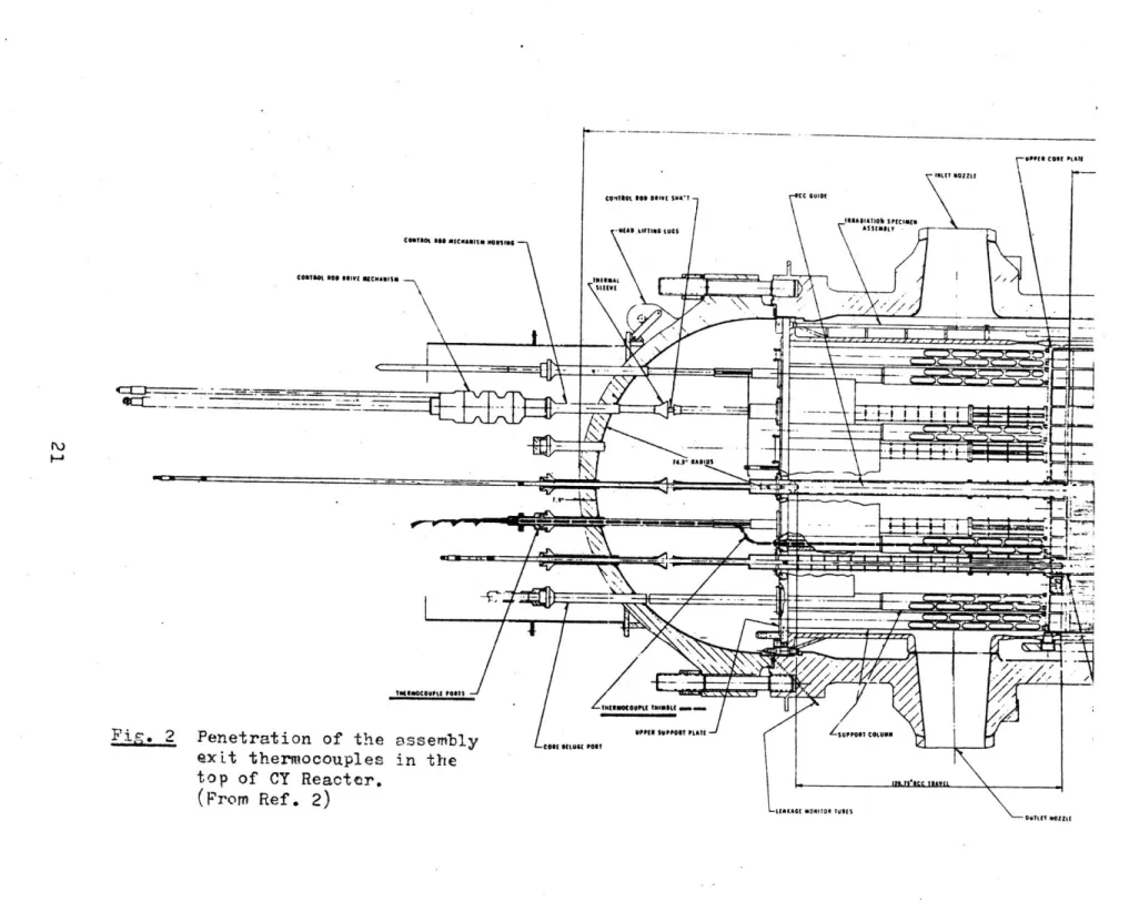
2 _{Penetration of the assembly exit 21}

thermocouples in the top of CY Reactor

3a Arrangement of the assembly exit 22

thermocouple on the upper core exit

3bc Details of the arrangement of the 23

assembly exit thermocouple on the upper core plate

4 Typical drive system for in-core 26

instrumentation

5 Arrangement of the movable flux 27

detectors in the bottom of the Connecticut Yankee Reactor

6 Comparison of the effective flow 34

factor calculation

7a Relative variation of F, H f'or 58

1% increase in the flux detector

readings. Assembly averaged values.

7b Relative variation of P , P H for 59

a' ,AH

1% increase in the flux detector

readings. Hot fuel rod values.

8 Typical example of the assembly 62

power not behaving as the general rule

9a Relative variation of F , AH for 64

1% increase in the flux thimble

prediction. Assembly averaged values.

9b

Relative variation of P

P

for

65

1% increase in the flux thimble

prediction. Hot

fuel rod values.

10

Model of the Connecticut Yankee

73

to be used in a COBRA III C

calculation

11

Comparison of outlet temperatures

82

as a function of the axial node

length

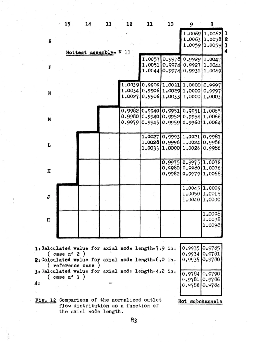
12

_{Comparison of the normalized}

₈₃

outlet flow distribution as a

function of the axial node length

13

Comparison of outlet temperatures

84

as a function of the flow

conver-gence factor

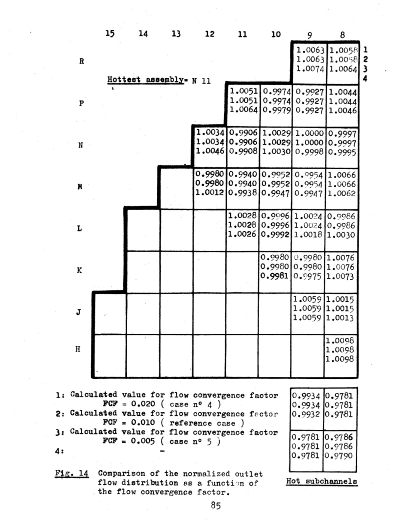
14

Comparison of the normalized outlet

85

flow distribution as a function of

the convergence flow factor

15

Comparison of outlet temperatures

86

as a function of the S/L parameter

16

Comparison of the normalized outlet

87

flow distribution as a function of

the S/L parameter

17

Comparison of outlet temperatures

88

as a function of the turbulent

momentum factor

18

Comparison of the normalized outlet

89

flow distribution as a function of

the turbulent momentum factor

19

Comparison of outlet temperatures

90

as a function of the cross flow

resistance

20

Comparison of the normalized outlet

91

flow distribution as a function of

the cross flow resistance

11

21

_{Comparison of outlet temperatures}

₉₃

as a function of the inlet

distri-bution

22

_{Flow distribution for the forced}

₉₄

inlet distribution case

23

_{Plow distribution for the equal}

₉₅

pressure gradient inlet case

24

Flow distribution for the uniform

96

mass flux inlet distribution case

25

_{Axial mass flux and cross flow for}

₉₉

the hot channel

26

_{Comparison of the axial mass fluxes}

₁₀₀

in the hot assembly and in the

assembly at the core center

27

Incipient boiling criteria applied

104

to the CY case

28

_{Coolant quality distribution at the}

₁₀₅

assembly outlet

29a

_{Fuel assembly (upper part)}

₁₀₇

29b

_{Fuel assembly (lower part)}

₁₀₈

30

Power distribution in the hottest

110

fuel assembly N

1.1

31

Coolant temperature distribution at

111

the top of fuel assembly N 11

32

_{Measured temperature rises, vs.}

₁₁₃

calculated temperature rises

33

Comparison of the uncertainties

123

associated with the effective flow

factors.

Heat capacity of the

coolant independent of the

tempera-ture.

12

34

Comparison of the uncertainties

124

associated with the effective flow

factors. Heat capacity of the

coolant temperature dependent.

35

Reactor cross section

126

36

Coolant temperature distribution

129

at the assembly exit. Power

increase in N 9 case.

37

Normalized flow distribution at

130

the assembly exit. Power increase

in N 9 case.

13

CHAPTER 1 INTRODUCTION

1.1 General Remark

The designer of a reactor is constrained by the re-quirement that the maximum values of certain design para-meters do not exceed critical values. Specific methods are used by the designer such as statistical treatment of hot channel factors, to evaluate the maximum value of a given quantity and the associated confidence level for not exceeding this maximum value.

The reactor operator is _{provided with different means}

of control, allowing either a continuous or a discrete

monitoring of the critical parameters that can be measured or evaluated from other quanitities. The goal is then, to achieve the production of the maximum thermal power, with-in the limits imposed by the technical specifications. From the reactor operation point of view, it is important

to know the actual values of the critical parameters and to see how they compared to the design values. It is

also important to include the fact that each parameter can only be evaluated within some uncertainty, since they are either measured or calculated.

The uncertainty in each value comes from the

in-accuracy of the control instruments, the inin-accuracy due

to the calculation method used, and even round off errors

due to the use of the computer.

For safety purposes, it is very important to always

maintain, an efficient capability for cooling the fuel.

The fuel temperatures should be kept as low as possible

for a given power level, including the hot spot location.

One factor in achieving this requirement is an adequate

coolant flow distribution.

This flow distribution depends on specific factors

such as:

_{the fuel bundle geometry, the pressure drop}

distribution, the coolant phase change, the power

distri-bution, etc. Most of the reactor manufacturers orifice

the lower core plate, which provides the fuel assembly

inlet distribution. The orificing is designed to yield

a rather flat temperature distribution of the coolant

across the core at the assembly outlet

.

Unfortunately the flow distribution among the fuel

assemblies cannot be measured directly. The problem is

even more complex in PWR's than in BWR's, since the PWR

fuel assembly is an open geometry assembly type allowing

flow and energy exchange between assemblies. In this

case the real flow is made up of:

- an axial flow which represents the most im-portant fraction of the total flow,

- _{a transverse flow or diversion cross flow,}

representing only a small fraction of the total flow.

As it will be seen later, the flow distribution can be related somewhat to the power distribution. The power distribution among the fuel assemblies is obtained by interpretation of axial neutron flux measurements in in-strumented assemblies. This evaluation depends on the accuracy of the flux detectors and the interpretative computation.

1.2 Problem Definition

This study has been developed to obtain a better under-standing of the effects of the various uncertainties in the control instruments and in the methods of interpreta-tion of the control data in terms of parameters such as

peaking factors, power distribution, effective flow factors. The data used throughout this study came from measure-ments taken at the Connecticut Yankee Reactor. They have been used to provide actual values of parameters for com-parison with the design values of these parameters. Period-ically, measurements are made in the Connecticut Yankee

evolution of:

- the power distribution,

-

the location and value of peaking factors:

EN

F

FN

- the effective flow factors.

The values obtained do not include the effect of

the different uncertainties due to the control instruments

or the calculation methods and are given in an absolute

manner. However, the limits are set to conservatively

include these uncertainties.

The problem is to evaluate the effect of these

uncer-tainties on the following quantities:

- _{local peaking factors,}

- _{effective flow factors,} - power distribution.

Table 1 summarizes the main characteristics of the

Connecticut Yankee Reactor.

1.3

_{In-Core Instrumentation of the Connecticut Yankee}

Reactor

The in-core instrumentation of this reactor is

de-signed to give information on:

-

_{neutron flux distribution using movable neutron}

flux detectors,

General characteristics Thermal power Electrical power Reactor manufacturer Number of loops (Mwth)

(MWe)

Number of fuel assemblies

Height of the core (in)

Mass flow for heat transfer (Mlb/hr)

Fraction of the total flow

by-passing the core

Fraction of the total heat generated within the fuel

Fuel design Fuel rod OD Pellet diameter

Active length of fuel 7uel array Fuel pitch Fuel type Table 1

(in)

(in)

(in)

(in)

:

1825

:

617

:

4

:

157

:

126.7

S

92.7

0.09

0.974

0.3835

:

15

15

0.563

Summary of the Main Characteristics of the

- fuel assembly outlet temperatures using Chromel-Alumel thermocouples,

at certain selected locations. Figure 1 shows the in-core instrumentation pattern. One may see that one quadrant

of the core is well instrumented, this assumes that the quadrant symmetry holds during the plant life, however, the octant symmetry which exists during the life of the first core, is no longer true after the first refueling.

1.3.1 Thermocouples

The forty-eight Chromel-Alumel thermocouples pene-trate the reactor vessel head through guide-tubes. The guide-tubes are located in some of the support columns which provide adequate rigidity for the upper core plate, whose main function is to hold in position all the fuel

assemblies constituting the core.

The thermocouples hot junction are located about

7 inches above the top of the fuel rods and about 13

inches above the top of the heated length. Figures 2

and 3a, b, c, show the thermocouples arrangement in the

Connecticut Yankee Reactor. When the coolant lives the top of the fuel rods it is channeled until it passes the upper core plat and the hot junction of the exit thermo-couple. Along this flow path, almost no cross flow

15 1413 12 11 10 9 8 7 6 5 4 3 2 1

IO

- I

1-r10r1

O O OI

I

0

0

1 1 1 1

_Ejma3F'~

b Incore flux detector

thimble location

0 Control rod bank A a Control rod bank B

Fig. 1 In-core instrumentation in the Connecticut

Yankee Reactor. (Fron Ref. 2)

0

LO O

SI

R

LO

0

0

0

MLO

O

ru

Fig. 2 Penetration of the assembly

exit thermocouples in the

top of CY Reacter. (From Ref. 2)

A

Opening in the upper core plate above an -unrodded assembly

-Fig. 3.a Arrangement of the assembly exit therrmocouple

A

Openingr in the upper core plate

aObove a rodded assembly

Fig. 34 and 3c Detail: of the arrangement of the assembly exit thermocouple Vnite uppTercr pa.

change with the other fuel assemblies takes place. There-fore the coolant flowing around the hot junction of the exit thermocouple comes only from the top of the fuel rods

of the fuel assembly below the thermocouple.

It is interesting to note that in actual operating experience it was not possible to easily replace the defective thermocouples, mainly because they are bent several times in the guide tubes. Design improvements have been made in future reactors so that replacement can be done with less problems.

1.3.2 Movable Miniature Neutron Flux Detectors

Two fission chamber detectors are used to measure the axial neutron flux. They are made of U₃0₈, enriched

at 90% in U2 3 5. Some of their characteristics are listed below:

Outside diameter: 0.188 in.

Length: 2.0 in.

Minimum neutron sensitivity: 2 x 1017 amp/nv Maximum gamma sensitivity: ₃ x 10 amp/nv

Operating thermal neutron 1 x 1011 to

flux range:

The two fission chambers are under remote control.

A complete flux mapping of the core takes about two hours.

Each instrumentation thimble in the fuel assemblies is monitored at least once by a flux detector. The neutron

flux detector is pushed by a mechanism up to the top of the fuel assembly. Then the detector is pulled, and while it is going from the top to the bottom of the fuel assembly, the neutron flux is recorded. This is done from the top, to be sure of the axial location of the flux detector

while the flux is being measured. Otherwise, if the flux

were recorded while the flux detector were moving from the bottom to the top of the fuel assembly, there would be a large uncertainty in the detector axial position. Figure 4 represents a typical drive mechanism for in-core movable flux detectors . Figure 5 shows a side view of the bottom part of the Connecticut Yankee Reactor (2) with the in-core instrumentation system.

During the flux mapping of the core, it happens that the flux can be measured several times at the same loca-tion by the two detectors (each enters the same flux

thimble at least once). This allows normalization of the two detectors, to account for the fact that they may not have the same cross-section or the same response for a given flux.

STORAGE REEL HELICAL-WRAP DRIVE CABLE DRIVE MOTOR 5-PATH ROTAGt'.' __ TRANSFER INTERCONNECTING TUBING WYE UNIT 10-PATH ROTARY TRANSFER ISOLATION VALVE HIGH PRESSURE SEAL SEAL TABLE DETECTOR

Typical Drive System for In-Core Instrumentation (From Ref. 4)

r\)

-J

Pig. 5 Arrangement of the movable flux detectors in the

bottom of the Connecticut Yankee Reator. (F'rom Ref. 2)

1.4

_{Other Instrumentation of the Connecticut Yankee}

Reactor

1.4.1 Limits of the Description

The description of the rest of the reactor

instru-mentation used at Connecticut Yankee, will be limited to

only the control instruments whose information will be

used in this study, i.e. measurement of the reactor

pressure, and coolant temperature at the vessel inlet.

1.4.2

Pressure Measurement

The reactor coolant pressure is measured on the

hot leg number 4, between the reactor outlet and the

stop valve. Two pressure transmitters are used:

-

_{for pressurization and depressurization, a}

0 - _{1,000 psig pressure transmitter,}

- for normal operation, a 0 - 3,000 psig pressure

transmitter.

Since the reactor coolant pressure is taken at a

location close to the reactor outlet, it may be assumed

that this pressure can be taken as the coolant pressure

at the core exit.

1.14.3

_{Inlet Temperature Measurement}

The reactor coolant temperature at the vessel inlet

is measured by a precision platinum resistance temperature

bulb located on each loop downstream of the steam genera-tor. Other bulbs of this type located upstream and

downstream of the steam generator give the loop average temperature and the loop difference temperature.

CHAPTER 2

EFECTIVE FLOW FACTORS

2.1 Definition

It was thought a few years ago, that the time evolu-tion of the "effective flow factor" (defined below) for a given assembly, might give some information on the time

history of the coolant flow in this assembly. Purther, by considering all the instrumented assemblies in the core, the effective flow factors might also give some indications

on the overall core coolant distribution. More precisely,

it was expected that a reduction of the value of the effec-tive flow factor in a given assembly, could indicate a

change in the channel geometry which caused a partial flow redistribution and a consequent change in the cross flow distribution.

To date only very small variations with time were observed among the effective flow factors, indicatinr that the channel geometry is unchanged, a fact which has been verified at each refueling.

In the assembly of coordinates I, J, the effective flow factor

EFPF*

* see Nomenclature of the terms used in this study in Appendix D.

- the ratio of the relative power q (assembly power/ core average power), to the coolant temperature axial rise At in this assembly, over the area of the core limited to the assemblies instrumented with an outlet

thermocouple.

where:

At = tou,1,j -tin,1, (2.1)

and the effective flow factor EFF is iven by:

38

EF

38

'

3

where 38 _{represents the normali ation factor over}

the area of the core limited to the assemblies instrumented with an outlet thermocouple which in the Connecticut Yankee

* The notation _{has the meaning of a sum carried over}

the instrumented assemblies in the instrumented quadrant (i.e., 38 assemblies).

case is the area of the core within the instrumented quadrant. This quadrant corresponds to the upper left quadrant on Fig. 1, which shows that 38 assemblies have outlet thermocouples. No credit is taken for the six remaining instrumented assemblies located in the three

other quadrants.

2.2 Assumption of the Effective Flow Factor

The above effective flow factor definition assumes implicitly the temperature independence of the coolant heat capacity. At a pressure of 2,000 psia a temperature increase of 50*F above an average temperature of 550'F (conditions which are typical of the Connecticut Yankee Reactor), produces a 9% variation of the heat capacity of the coolant.

The temperature dependence of the heat capacity of the water can be taken into account in the computation

of the effective flow factors, by replacing the temperature rise

At i

Ah

_i,j

_ou,i,j

in,i,j

Similar definition of the effective flow factor will lead to:

EFF = h

x

38

For the same collection of data (relative power distribution and temperature rise distribution), the comparison between the two values of the effective flow factor for a given assembly shows:

- the effective flow factor using the temperature rise is generally not as close to 1.000 as the effective flow factor using the enthalpy rise (a difference of the order of 1% or less).

This comparison is summarized in Fig. 6 for data collected at BOC in Core III. Other comparisons done in Core I and II (not presented here) agree with this observation.

2.3 Sensitivity Analysis

Since the effective flow factors are computed from measured and calculated values, it is interesting to

determine the contribution of each value used in the calcu-lation of these effective flow factors. In particular

the evaluation of the accuracy of the effective flow

-UOT~a1UOTO J0O!-01'J 4013 OAIT.OOJJO9q . JO U0STJadwoo)9 1i

~

o

)

3

)

9eC6*o

Vii101 9TL6*O

!4fo

L96

TL6?"

i

C4

I

C760

FIiE6o0 tz1lo

6C96oo eOt'OT

V99050

o6ZT

61CoOT oVC6o

0Q9- 1

?fO'TI

9o 9Za1.I

LL6o0

66T*T

L 6*0

961

00oLV

OE'*

0009V

O902

09C

OC04

OZO04

O19tV

9fZOT 9600o1

otVO*T

6Kvoll

6Z O*T1o6*o

O9tVOt

9ffOMl TOOT

tTFO4C OT

I L6900

9ZOIl

9Z6O0

LUVI

01

9COT

ITLOO

oL,,C4

o66l

poq

-1-OT9

Olt2

Otil0

T9tT*

£01.1

9V~6600

Cf66*0

09690

o1II

E

TL

Ca

*

TEt

6z6oo

otCo'T

OW

LT

q*0,90

£

OT TZ96o

£ 66o0

O1L6

z6g6oI ZT9o.T

iZUf~o

9000.1T 9TLoOT

9ZLO

9 06-O

LT96o0

MWT7Y

Co~eo

990*T

9960

L6*

6o

Z91-1

9EZ"T

60LoO

0t194~~~~~

-

0~

0C

o.I9r

LLgooT

0lTg190

190900

09L0O

09*

LLooO

9910"

L

SA@'

09TO0T

0991 " T

L6

T*T

9969r 0

T0060o

iC6O

09

6620oT

LREo*T

9LT-0171 9

LIMV6lo

9T46*o

290T

0t

109

o6L~o

06 "617

K

"IzL6*o

6 96

1o

06"

9

99ZOO

ZIO0*

9V1*

Eg

l9

£TI

0

9909*0

-al

TT

XN7"e

.516

6

t

TT

cr [

T

9T

r

()

11

H

U

%

6

ri

factors and the breakdown of this accuracy due to the relative power distribution and temperature rise distri-bution gives a better understanding of the problems

re-lated to the in-core instrumentation.

2.3.1 Sensitivity Analysis for Constant Heat

Capacity of the Coolant

The effective flow factor is given by Eq. 2.2, which can also be written as:

EFF = At x k, (2.5) where: k = 38 (2.6)

Z

±

Ij

arq1j = relative standard deviation of the relative power,

at = standard deviation of the assembly outlet temperature,

at in,=,j standard deviation of the assembly inlet

temperature.

The square of the relative standard deviation of the effective flow factor is given by:

38

At

1,

j

i,

_(2.7)

The square of the standard deviation of the effective flow factor is given by:

2EFF i

2

1,j

(2.8)

* _{See Appendix E for the derivation of Eqs. 2.7, 2.8,}

38

1 1,

component due to the

normalization

k

2

2

2

+ja

q

₁

q.

_{component due to the}

'J

rpower

_distribution

+

[k

]

2t

+ A2t t ou,1

ij

component due to the outlet temperature

[

_At

j

, 2 icomponent due to the

inlet temperature

(2.8)

(continued)

But the component due to the normalization can be split into:

[]2

ti

][2

38

4\1,

37

(2.9)

2i

2

[AtjA

2

2r

qj

A2

otin

At

_term due to the power

term due to the outlet temperature

term due to the inlet temperature.

(2.9)

(continued)

The total contribution of the power distribution, the outlet and inlet temperatures is the sum of the corresponding terms in Eqs. 2.8 and 2.9.

A code called FLOFA I has been written to calculate

the standard deviation on the effective flow factor (see Appendix B for the code listing and sample input and

E

output). From the data, relative power and temperatures

distributions, the code is used to compute:

- _{the effective flow factor distribution,}

- the standard deviation of the effective flow factor,

- the breakdown of the square of the standard deviation of the effective flow factor into components due to:

- normalization,

- power distribution,

- outlet temperature,

- inlet temperature.

This is done for assumed values of standard deviation on relative power distribution and inlet and outlet tempera-tures. These values can be varied by the user.

2.3.2 Sensitivity Analysis for Temperature

Dependent Heat Capacity of the Coolant

Similar work has been done in this section as in

2.3.1. By using Eq. 2.4 to define the effective flow

factor:

q

38q

EFF = 38 = qih x kt (2.10)

i1,j

qh1,j

where:

38

kt

38

The square of the relative standard deviation of the effective flow factor is given by:

38

a2

a2

qij

r

,j

-3

(2.11)

* See Appendix E for derivation of Eqs. 2.11, 2.12, and

2.13.

The square of the standard deviation of the effective flow factor is given by:

2

2

38

a2

t

x

a

(

. )

i

qL,

iJ%1

{component

2

[+

2

2

+

[Aht1

r

1,j

,

component due to

the power

1

2

2

oh

_t

_j

ou,i,j

_{(component due}

to the outlet

temperature

in~iJ

_{component due}

to the inlet

temperature.

(2.12)

Splitting the component due to the normalization

would lead to:

2

38

A2

c2

2

2

38

2

38kt

Ni

ar

ou.

iIj~

tou ,

i

,j

at

ouij

21

.ou,i

.,j

term due to the power

term due to the outlet temperature

(h

2

at2

S

in,,j

h

2

term due to the

inlet

temperature-(2.13)

(continued)

The above derivation assumes that the coolant stays

subcooled and the evaluation of oh can be obtained from:

2

rahi 2

t

oh

t

(2.14)

A code called FLOFA II has been written to compute

the same information as FLOFA I (see 2.3.1) with the

effective flow factors obtained from the enthalpy rise.

(see Appendix B).

2.3.3

Evaluation of Uncertainties

In order to calculate the uncertainties associated

with the effective flow factors, it is necessary to have

the values of the control instrument uncertainties

(thermocouples, flux detectors).

Research done in this

area showed that very little data exists.

Thermocouples:

The assembly exit thermocouple is made with

Chromel-Alumel. This type of thermocouple has a good resistance to radiation damage and has a characteristic

curve which stays linear with time . However

the accuracy of this type is not very good. The standards of the American National Standard Institute require that the thermocouple manufacturers meet the following specifi-cation for the Chromel-Alumel type:

- for temperatures between 0 and 530*F

- limits of errors of standard thermocouple + 4*F

- limits of errors of special thermocouple + 20F - for temperatures above 5304F

- limits of errors of standard thermocouple + 0.75%

- limits of errors of special thermocouple + 0.375%

However these standards do not indicate the

confi-dence level associated with these values of possible errors. In fact this gives only a value of the thermocouple uncer-tainty due to the reading accuracy. Other values of un-certainty need to be found concerning:

- _{calibration error,}

-

hot junction drift due to nuclear permutations,

- hot junction position with respect to the center

of the fuel assembly.

A study done for the San Onofre Reactor

gives

some numerical values for the different uncertainties:

- calibration error (statistical) evaluated as + 0.3*P

which is due to the fact that the isothermal

cali-bration of the thermocouples is done at an average

temperature of 530%F which is about 40OF below the

operating temperatures of the thermocouples (a check

on the calibration curve of the thermocouples shows

that the correction at 530*F is the same at 570-5800F).

This calibration error is used to take into account

also a possible human error and is conservative in

that respect,

- _{gamma heating (non-statistical) evaluated as + 0.5}0

_F

to take into account absorption of gamma rays energy

by the hot junction at full power which gives higher

readings,

-

_{hot junction drift due to nuclear permutations}

(non-statistical) evaluated as +1*F.

The records concerning

the thermocouples off-sets for Connecticut Yankee

Reactor between two isothermal calibrations, show a

maximal drift of 1.55*F in Core III (1.754F in Core IV)

and also show that these drifts may occur in opposite

directions, which indicates that this error is of a

non-statistical character,

-

hot junction position with respect to the fuel assembly

(statistical) evaluated as

+

3

F. This tends to take

into account the fact that the coolant temperature at

the plane where the temperature is taken, is not

uni-form,

-

reading accuracy (statistical) evaluated as

2.04F

due to the instrumentation.

The vessel inlet temperature of the coolant is

measured by a precision platinium resistance temperature

bulb in each loop. This type of instrument can be used

in this case because the hot junction is not exposed to

the full neutron flux and the exposure damage is less

in this case than for the exit thermocouples. Based on

the engineering experience, it is common to consider an

inaccuracy of

+

0.2

F associated with the reading of such

RTD (Resistor Temperature Device).

Power Distribution:

The movable miniature flux detectors are supposed to give their signal with a + 2.0% accuracy and Westinghouse estimated the accuracy of the power map on the order of

+ 5% Both values are related to a two sigma confi-dence level.

2.3.4 Results of the Sensitivity Analysis

At the time the sensitivity analysis was developed,

the uncertainties associated with the control instruments were not known with enough precision, and the standard

deviations of the effective flow factors were calculated with assumed values for these uncertainties, based on engineering experience and Judgment.

The results obtained assumed for the one sigma

con-fidence level:

- _{relative standard deviation of the power: 0.0275} - standard deviation of the outlet temperature: 2.50*F

- standard deviation of the inlet temperature: 0.10'F For the one sigma confidence level the relative standard deviation of the effective flow factor was in the range 4.5 - 7.0%, and was an inverse function of the

coolant temperature rise in the fuel assembly. The

tive standard deviation of the effective flow factor is also strongly influenced by the standard deviation of

the outlet temperature as it can be seen on Table 2. Table 2 gives the breakdown of the standard deviation of the effective flow factor and the comparison between

the two types of analysis (C temperature dependent and

p

independent).

2.4 Physical Meaning of the Effective Flow Factors

If no cross flow between the assemblies is assumed,

it is _{obvious that in this case the effective flow factor}

is the same as the normalized inlet flow distribution.

But the real case of PWR is more complex and the assumption of no cross flow does not necessarily hold.

The energy equation can be written as:

C (m _+Am

)tou,1.j - C min,1,j t

iQj - Cp Am

iti.

where ti represents the effective temperature for the energy due to the cross flow exchange,

C

Type of case

Four components due to: - normalization factor

- power

- outlet temperature

- inlet temperature

Three total contributions due to:

- power - outlet temperature - inlet temperature

C =constant

p

2.60

%

23.38

~

73.91

0.11

100.00

24.00

_%

75.87 %

0.13

%

100.00

%

p

30.09

/

67.17

%

30.88 /

68.97 %

Breakdown of the Standard Deviation of the Effective Flow Factor for BOO in Core TIT of Connecticut Yankee Reactor

49

Solving for min,1,j we obtain:

m ii

QiJiC

-

Am

i

(ti'i

+

t

j)

-

(2.16)

oujj - tinij

And if these ratios are normalized over the area of

instrumented assemblies:

Qi

j

- Am

(t

+t)

E

F

F

_o

u ij - t

_{i n}

_i

(2.17)

38

Min,i,j

A similar equation can be derived for the case where

the heat capacity of the coolant is assumed to be

tempera-ture dependent.

The evaluation of the term corresponding

to the energy exchange between the assembly i,j, with its

neighbors can be reduced to a net energy exchange which

corresponds to a cross flow exchange and thermal mixing.

It i rather difficult to evaluate this net energy exchange,

because it implies knowledge of the temperature or

enthalpy distribution along the fuel assemblies and also an idea where the cross flow exchange takes place. One way to get the feeling for this process is to run

calcu-lations with a thermal hydraulic code like COBRA III C which yields the temperature enthalpy axial flow and cross flow of the coolant. Results of this type of

CHAPTER

₃

POWER DISTRIBUTION CALCULATIONS AND USE OF THE CODE "INCORE"

3.1 Introduction

The power distribution and the corresponding peaking

factors FN

_{H' q'q}

F

N Fq, are calculated by the code INCORE.

This code uses as main inputs:

-

the flux detectors readings measuring the axial flux

in the assemblies instrumented with an in-core thimble,

and the flux at each thimble location,

-

the prediction of the core wide power distribution

and flux thimble obtained from the code PDQ

(11), in

which the results of depletion calculations using

the code LEOPARD(

), are fed.

In the Connecticut Yankee core there are two flux detectors

which can be moved within all of the 18 flux thimbles

located in 18 different assemblies.

The power distribution calculations using the computer

code PDQ, is generally done stepwise each 2,000 MWD/MTU.

Some of the INCORE results are used to determine the:

-

maximum linear heat generation rate and its location,

- _{average linear heat generation rate,} - _{peaking factors and their locations,}

3.2

Purpose of the Calculation

A sensitivity analysis has been developed for the

code INCORE for two purposes:

-

_{it was found interesting to know the sensitive effect}

of the major inputs on the results, since no

informa-tion so far, was not readily available on this type

of analysis,

-

the sensitivity analysis is needed for good

informa-tion on the accuracy of the results of the power

distribution calculations from the knowledge of the

inputs accuracies.

The code INCORE is a proprietary code from Westinghouse,

and information beyond input and output is not included

in this study.

3.3

Modification of the Major Inputs

As mentioned in 3.2, because of the proprietary

character of INCORE, no numerical values relative directly

to the inputs or outputs are given in this work. But to

understand what has been done, some explanations are given

how the inputs have been treated.

The sensitivity analysis has been developed from the

variation of:

-

flux detectors readings given by the movable incore

flux detectors,

- PDQ flux predictions of the flux at the flux thimble

locations,

- _{power distribution prediction given by the PDQ code,}

for hot channel and assembly.

This study, of course, uses numerical values of the inputs for a given cycle, at a given time in the cycle, however the time effect has been considered. The

para-meters were varied one at a time, to see their corresponding

effect on the entire output.

3.3.1 Variation of the Flux Detector Readings

For a given thimble, the detectors readings have been varied by the same factor (5% increase has been used to be sure of having enough variation in the outputs without too much distortion of the power pattern).

It has been verified for the first thimble, that an increase and a decrease of the flux detector readings by the same factor, would give output changes equal in abso-lute value. This was done to check that the change was small enough to be considered a linear effect.

3.3.2 Variation of the Flux Thimble Information This part of the sensitivity study was treated in a very similar fashion as for the flux detectors readings. For a given thimble, both the thermal flux information and the fast flux information, were varied by the same factor

(5% increase has been used for the same reasons as 3.2.1,

after having verified the linearity of the changes in

the outputs with the changes in the inputs).

3.3.3

Variation of the Predicted Power

The sensitivity analysis for this part has been

con-ducted in a different way, because for a given cycle the

power distribution changes only with time. Therefore,

comparisons have been done between collection of power

predictions at BOC, MOC and EOC of CORE III.

3.4

Results of the Sensitivity Study

The results of this study depend upon the kind of

input that has been varied. The results are presented in

a relative value, expressing the percentage change in the

assemblies for a change of one percent in a given location

for a given type of input. To handle the calculation of

the variations, a code VARY has been written and all the

details are given in Appendix B. All the results have

been summarized in curves for easy use.

3.4.1 Variation of the Flux Detectors Readings

The increase of the flux detector readings in a given

flux thimble, gives the following results:

-

FN

F are increased locally by variable amounts

de-pending on the relative position of the assemblies

with respect to the location where the increase takes

place:

- _{for the assembly in which the increase is made,}

F'1 F are increased by almost the same amount

(1% increase of the flux detector readings gives

0.9% increase for F NH and F ),

- for the assemblies immediately surrounding the assembly where the increase is made, FN F are

AH'

q

- FNH, FN are decreased throughout the rest of the

AW q

core by a fairly constant amount,

- Fz is unchanged.

Figure 7 summarizes the results of flux detector, giving the relative variation of F H or F normalized

AH

q

to a percent increase in the flux detectors readings as a function of the radial position of the assembly from the center of the core and as a function of the position in which the increase in the flux detector readings takes place.

Key to Pig. 7a, 7b, 9a, 9b

Curve A = relative variation of the peaking factors for the assemblies which are not the neighbors of the assemblies where the variation (flux detector readings or flux thimble prediction) is done,

(assembly case 1)

Curve B = relative variation of the peaking factors for the assemblies sharing a common corner with the assemblies where the variation is done,

(assembly case 2)

Curve C = relative variation of the peaking factors for the assemblies sharing a common side with the assemblies where the variation is done,

(assembly case

3)

Curve D

=

relative variation of the peakinq factors for

the assemblies where the variation is done,

(assembly case 4).

Radiale distance from core center

=

distance between the

center of an assembly and the center of the assembly H 8.

assembly

case

1.

01assemhy

case

3

assembly case

4

Relative voraEon of

2 Fg F " far I-he assembly 1.040 .9

[

Prom core center

.0 0 0 0 C

8

-- - -- -~ ~

A-,

Fig. 7a Relative variation of F F for 1 increase in thei flux deteetor reaings.

60(;n) \-n co 0.6 0.5 - 0.4- 0.3-0.1 0.0 -0.1 0 (pil-ches) I I I I

Re IcAhve vari;a;on oF

N N

F F Wor

the

2 9' AH

(1o I

ui

20 30 40

Raccial dis tauce

From core cenler

50

0 10 20 30 40 50 60 70 80 90 400

N N(ichs

Fi. 7b Rlative variation of F for I o increase in the flux detector readings Hot fuel rods values.

As an example, an increase in the flux detector reading of 1% in assembly M10 (radial distance

67.08

- increase of FAH or FN of: 0.42 in N 10 (radial

AH

q

distance = 80.78 pitches,

sharing one common side with M 10, curve B)

0.32 in N 11 (radial

distance = 87.46 pitches

sharinit one common corner with M 10, curve C).

Now it should be mentioned that INCORE computes the power distribution from the flux detector readings, and the number of thimbles used for the calculation of the power in a given assembly, apparently may vary from 1

to several thimbles.

It has been found that the curves of Fig. 7 are time independent for a given core, a given assembly has its power changing with burn-up, however the relative variation of FAH or F stays constant while burn-up

AH

q

increases.

Some of the calculated relative variations of F N

_AH

or F N may not behave as shown in Fig. 7. This is appar-ently due to the way INCORE treats the problem and it

has been found that the calculated power is inferred from the information related to a fairly far thimble as shown in Fig. 8. For this case there has been a one percent increase in the flux detector readings in M 12 and the corresponding variation in N 12 should be 0.73

according to Fig. 7, but instead it is - 0.028 corresponding

to the variation of the rest of the core. This is due to the fact that the power in N 12 is given from the informa-tion in L 5, which in this case does not see the effect of the one percent increase in M 12.

3.4.2 Variation of the Flux Thimble Prediction Very similar results have been obtained for this part as in 3.3.1, except that in this case the variations

of F H and F are in the opposite direction to the way they varied in 3.3.1.

The increase of the flux thimble prediction in a given thimble, gives the following results:

- FN F N are decreased locally by variable amounts

AH'% q

depending on the relative position of the assemblies with respect to the location where the increase

takes place:

N

- for the assembly where the increase is done, FAH' F are decreased by almost the same amount,

q