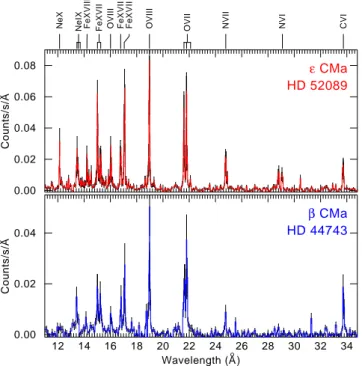
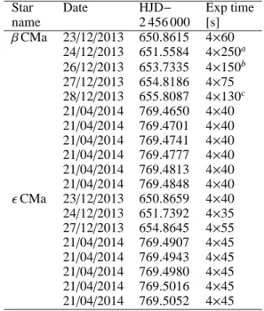
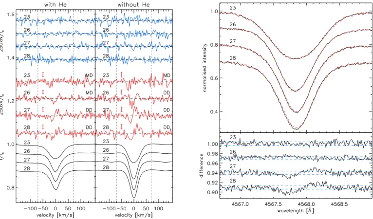
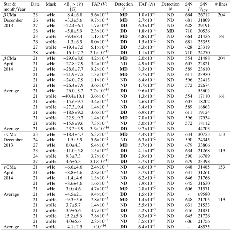
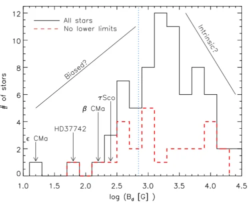
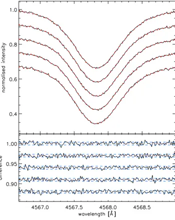
B fields in OB stars (BOB): on the detection of weak magnetic fields in the two early B-type stars beta CMa and epsilon CMa
Texte intégral
Figure
Documents relatifs
Dans le cadre du projet Jangkrik la partie technique du projet est assur´ ee par deux (2) sp´ ecialistes (hardware et software) qui se basent sur les documents d’entr´ ees fournis
Revenu total du ménage agricole Retraits Autres revenus Revenu d’emploi extérieur Revenu d’activités para-agricoles Paiements directs Revenu agricole Revenu brut Avoir
Dans cette partie nous allons voir comment nous sommes passés d’un moyen de mesure manuel à une solution de test automatisé en examinant les deux points cruciaux qui
En este sentido, se observa que se subestima el potencial de Internet, la web y las redes sociales en relación a la promoción turística, ya que, aunque todos los museos entienden
In the field, by using a regression between measured value and reference values, the LAI could be estimated with a standard deviation of 0.39. This was higher than the
Avec les auxiliaires de puéricultures, nous avons au fur et à mesure eu le même questionnement : maintenant que nous savons comment s’adresser à Amadou pour qu’il nous
Ainsi, nous retrouverons le festival Le Grand Rassemblement, comme projet phare de la structure, mais également d'autres actions de médiation, notamment en
Dans le cadre d’une campagne de prévention, un dépistage du diabète a été proposé aux personnes n’étant pas sous traitement anti-diabétique, mais présentant un risque
