ASSESSMENT OF PLANT LEAF AREA MEASUREMENT BY USING STEREO- VISION

ASSESSMENT OF PLANT LEAF AREA MEASUREMENT BY USING

STEREO-VISION

Vincent Leemans, Benjamin Dumont, Marie-France Destain

Gembloux Agro-Bio Tec – University of Liège

ABSTRACT

The aim of this study is to develop an alternative measurement for the leaf area index (LAI), an important agronomic parameter for plant growth assessment. A 3D stereo-vision technique was developed to measure both leaf area and corresponding ground area. The leaf area was based on pixel related measurements while the ground area was based on the mean distance from the leaves to the camera. Laboratory and field experiments were undertaken to estimate the accuracy and the precision of the technique. Result showed that, though the leaves-camera distance had to be estimated precisely in order to have accurate measurement, the precision of the LAI evaluation, after regression, was equivalent to the reference measurements, that is to say around 10% of the estimated value. This shows the potential of the 3D measurements compared with tedious reference measurements.

Index Terms— LAI, 3D, plant leaf area, ALA. 1. INTRODUCTION

Leaf area index (LAI) is an important property of vegetation, since it determines the photosynthetic primary production, the plant evaporation and characterizes the plant growth. The LAI considered here is the total one-sided area of the leaves per unit ground surface area [1]. The reference measurements for the LAI of crops are destructive, tedious and expensive. Indirect methods have thus been developed and Jonckheere classified them between those based on the absorption of radiations by the leaves and those based on the gap fraction [1]. Bréda specifies the exponential relationship between the LAI and the gap fraction [2]. This function must be known or estimated before computing the LAI based on the gap fraction. Aparicio described methods based on canopy transmittance or on the reflection in specific wavelengths such as the “Simple Ratio” or the “Normalized Difference Vegetation Index” (NDVI)[3]. The inconvenient of those methods is to be influenced by the chlorophyll content or the soil type and to saturate when the soil is completely covered. Kirk et al. proposed a LAI evaluation method for cereals using images acquired by a colour camera from above the canopy [4]. The gap fraction was measured and the LAI was computed by adjusting an exponential canopy model. The model returned the gap fraction in function of the LAI and the mean leaf angle. Once fitted it was inverted to estimate the LAI. Author took

into account varying zenith angles thorough the image. The method was compared with destructive reference measurements and with the measurements obtained by using LAI-2000. Results showed that the LAI-2000 gave a slightly better correlation (0.78-0.90) with the reference compared with the camera (0.68-0.81). Different authors stressed the importance of the zenith angle to measure the gap fraction and the interest of a zenith angle of 57.5° [4-5]. Several commercial instruments for measuring LAI are cited in literature [1], [2], [6]. They are based on the same principles (extinction method, gap fraction from different incident angles). All these instruments are not suited for measurement of crops during early developments (LAIs <1), while cameras can be used at that stage [4].

In agriculture stereo vision has been used to enhance weed vs crop recognition, with the aim of guidance or for animal or plant shape evaluation. Andersen et al. used stereo vision for three-dimensional analyses of single plants [7]. They focused on the use of simulated annealing as a robust approach for pixel-to-pixel correspondence between left and right images. They were able to reconstruct the plant geometry and to measure plant height, leaf angular distribution and leaf area.

This paper presents a non-destructive and low-cost method using a vision camera set-up. Because stereo-vision is able to extract three-dimensional leaf geometry, assumptions or estimations about the leaf angle distribution are not required for the proposed technique. The average leaf angle (ALA) is another related parameter of interest which could be determined using the same technique. The precision of the leaf area measurement was assessed with references during laboratory tests and then validated with field acquisition compared with destructive measurements data.

2. MATERIAL AND METHOD 2.1. Material

The devices used in the experiments are twin colour CMOS cameras model STH-MDCS2-VAR-C from Videre Design (CA, USA) having sensors made of 2048*1536 pixels. Images could be acquired either down-sampled at a size of 1024*768 pixels or at full resolution but from a sub-region (1280*960 pixels) of the sensor. The camera couple were observing the crop from around 1 m for the 1024 image width and 1.3 m for the 1280 width. The two points of view

were distant of 115 mm. The focal lengths were 16 mm and the optics were equipped with an IR-cut filter. A vergence of 4.5° was applied to the system to maximise the area inspected simultaneously by the two cameras. The cameras were observing the plant with their medium optical axis presenting a zenith angle equal to half the vertical angle of view (15°), so that the bottom part of the images was viewed from the zenith. The field stereo images were acquired, saved in “tiff” files and processed off line. The camera drivers were the CMU 1394 Digital Camera Driver from the Robotic Institute, Carnegie Mellon University.

2.2. The crop and the reference measurements

In order to evaluate the precision of the 3D method, 3D field measurements were compared with 3D references. The field experimentation concerned wheat (Triticum aestivum L., cultivar Julius) and was part of a more complex set-up aiming at the determination of the dry matter and grain production of wheat in function of the nitrogen fertilisation level. For this experiment, two fertilisation levels were applied (0 and 180 kg N/ha) and there were four spatial repetition for each and five images couple were acquired per plot, on the 8th _{April, 6}th _{May and 4}th _{June 2013. The}

nitrogen fertilisation and the dates were useful by providing a variety of LAI values and the different growing stages.

The reference measurements for the LAI were computed by harvesting the plants in 0.5 m of a line in each plot. The stripped leaves were stuck on a paper sheet and scanned. The images were segmented (colour threshold) and the area was measured and the result extrapolated for a square metre. Because it was hardly possible to measure the reference LAI and the 3D-LAI on exactly the same spot and because there were more 3D measurement, the comparison between the 3D and reference LAIs was made on a statistical basis.

Moreover, to assess the repeatability of the 3D measurement, on one plot, five image were acquired at exactly the same spot so that the only differences were due to the wind and to the measurement noise.

2.3. Evaluation of the leaf area measurement precision by using patterns.

This experiment was aimed at evaluating the accuracy and the precision of the proposed area estimation method. Patterns having known “leaf” area were presented to the cameras at different distances and different angles. The deviation of the measure with the true value (accuracy) and the standard deviation of the measure (precision) were assessed. The relation between area and the leaf width, the distance from the leaf to the camera and the angle between the optical axis and the leaf plane were also evaluated. The two image widths were tested (1024 and 1280 pixels).

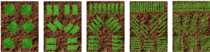
The patterns consisted in printed images containing a soil image background and rectangles showing leaf areas (Fig. 1). The patterns were composed of six “leaf” squares or a multiple of six rectangles with decreasing width (respectively 1/2, 1/4, 1/8, and 1/16 of the square width) and different orientation. All the patterns present the same “leaf” area, 0.01551m². The images were composed by

using Gimp and the reference area was measured by using Image-Pro (Media Cybernetics). They were printed using a resolution of 200 dots per inch. For each pattern, nine images at different distances from the camera (from 0.9 up to 1.7 m) and different angles between the optical axis and the image plane were acquired (45 image couple for each resolution). The distances from the optic to the pattern (in the centre of the image) were measured and used to control the calibration.

Fig. 1. Different patterns used for the area evaluation. 2.4. Stereo images processing

The stereo images were processed by using OpenCV libraries. By convention, the “real dimensions” symbols are noted with capital letters and expressed in metres while their digital counterparts are expressed in pixels and are noted with lower case.

The 3D system calibration to fit the internal parameters (camera linked such as focal distance or distortions) and external parameters (distance between camera, vergence, …) was carried-out indoor, before the acquisition using a chequerboard and by using the appropriate OpenCV libraries (2.3), as described in Bradski and Kaehler [8].

The same processing was applied to the images acquired in the filed (2.2) and to those acquired in the laboratory (2.3). It comprised several steps : computing the 3D coordinates of each pixel of the image, the plant vs soil segmentation, the measurement of the observed ground area, and the computation of the 3D areas of leaf pixels.

For the 3D coordinate computation, the first treatment was a geometrical rectification and the computation of the disparity by using a modified H. Hirschmuller algorithm (StereoSGBM). This algorithm involves several parameters. For several of these, the default values were not the best ones because the objects in this application (leaves) were of small size. The “matched block size” was fixed to 5 pixels, the “uniqueness ratio” was fixed at 10 percent and the “speckle window size” was of 50. The algorithm research for the disparities from a minimal value noted m and in a range noted n (both in pixels). Fig. 2, bottom left, presents a map of the disparities for the two above images.

By using the calibration, the pixel disparities were converted in camera-linked three-dimensional metric 'XYZ' referential with the origin centred on the sensor, the 'Z' coordinate pointing from the objects to the camera.

2.5. Leaf area estimation

The algorithm also returns for the reference image (the left one) the position and the dimensions (noted xROI and yROI,

wROI, hROI) of a rectangular region of interest where the

density varied perpendicularly to the plant rows, it was important to consider an entire number of rows (vertically in the images – y axis). A region within the ROI was thus defined, here after referenced as the Region. Its horizontal dimension was w (in pixels) and its height h.

Fig. 2. Example of images acquired and result of the

treatments. Above left and right images after geometrical rectification. Below left the disparities, the pixels closer to the camera being lighter grey. Below right, the result of the leaf/ground segmentation (leaves in white).

The dimension of the Region, w and h, converted into the real XYZ metric dimensions, were used as soil area measurement for the LAI. It was computed based on the mean distance from the camera to the leaves Zm, from the

focal distance and from the sensor characteristics. The total area was given by :

At=h⋅w⋅

(

(

)

)

2

(1) with P the pixel pitch in metres and F the focal distance of the optic in metres. The observed area At was around 0.13

m².

In a next stage, the plants were segmented from the soil in the left image by linear discriminant analysis applied on the RGB colour parameters of the pixels (Fig. 2 bottom right).

Then leaf area was evaluated for each triplet of adjacent pixels included in the Region (noted A, B, C, Fig. 3) and belonging to the leaves. This includes the computation of the cross product (CP) of two vectors joining the summits of the triangle in the XYZ coordinate system :

⃗

CP= ⃗

AB× ⃗

AC

Fig. 3. Representation of a leaf image pixel, with pixels A,

B, C and D used for the local area computation. At the bottom the four possibilities to draw triangles in a square are shown. For sake of clarity, only the left one (ABC, ACD) is represented above. Clearly, the ABC, ACD set is better suited for the represented leaf orientation.

The direction of the perpendicular to the local leaf plane was given by the resulting vector and the area was given by half its module. The total area of plant leaves was computed by summing the local areas over the Region. But in a square composed of four adjacent pixels, it is possible to draw four triangles (ABD, ACD, ABC, BCD, Fig. 3 bottom). If the four pixels belonged to a leaf, the area of the four triangles were computed, added and the sum divided by two :

A

=1/2

∑

Triangles

∥ ⃗

CP∥/2

Otherwise, if three pixels belonged to a leaf, the area Al was

the area of the triangle. The ratio of this sum to the Region soil area gave a measurement of the leaf area index :

LAI=

A

A

This LAI will be referred to 3D-LAI. The angle  between

⃗

CP _{vector and the Z axis was given by :}

α=

acos

(

CP

∥ ⃗

CP∥

)

The mean of this angle for the ROI gave the average leaf angle (ALA).

Fig. 4 shows the representation of Fig.3. but seen from a different angle than the optical axis of the camera. The true position of triangle ABC has been represented in doted lines while the measured one are in solid lines. The effect of the random error will be discussed in the next section. The light green triangle show three adjacent pixels belonging to two different leaves, presenting different elevations. The inclination of the triangle with the optical axis is important and the area would be clearly over-estimated. To avoid this problem, the data from the triangles presenting a cos(α) (Eq. 5) below 0.2 were not considered.

D C B A C A D B B A C

Fig. 4. Representation of leaf image pixels as in Fig.3. but

seen from a different angle than the optical axis of the camera.

3. RESULTS

When comparing the distances between the cameras and the patterns, measured by using the 3D cameras with references measurements, the correlation coefficient was 0.9997 and the slope was 1.0003 showing that the 3D technique was able to measure distances accurately (Fig. 5).

Table 1 shows the accuracy and the precision of the estimated “leaf” area. The relative accuracy is expressed in percent of the reference value (0.01551m²) and the relative precision is expressed in percent of the mean value.

Table 1. Accuracy and precision of the area measurements.

Image sizes 1024*768 1280*960

relative

(%) m² relative (%) m²

Accuracy 34 0.0053 49 0.0075

Precision 10.9 0.0017 15.8 0.0024 Both image sizes present an over-estimation in the measure of the area. It was more important for the bigger images. The error in the measurement of the area came from errors in the estimation of the distance from the camera to the area observed by each pixel, but the responses to systematic and to random error were different.

Systematic error impacted the area according to Eq. 1 for the total area and to Eq. 3 for the leaf area. The three components of vectors AB and AC (Eq. 2) are proportional to the distance camera-object for the X and Y components and to the difference between those distances for the Z component. Thus both areas are directly affected by an error in the estimation of Z. However, the LAI being the ratio of these areas remains unaffected by such an error. Moreover, it has been shown that the ratio estimated

distance/reference distance was pretty close to unity. The exaggeration observed in the area measurements was thus not linked to a systematic error.

0,8 1 1,2 1,4 1,6 1,8 0,8 1 1,2 1,4 1,6 1,8 1024 Regres (1024) 1280 Regres (1280) Estimated distance 3D (m) T ru e d is ta n ce ( m )

Fig. 5. relation between estimated and reference distance

between an object and the camera.

The situation was different for the random errors. When measuring the triangle areas, any error in the evaluation of the distance camera-object modified the Z coordinate and thus changed the orientation of the triangles in ABC. Because the reference area was a plane and when the optical axis was almost perpendicular to it, this tended to increase the area of each individual triangle compared with the reference. Estimation of this exaggeration based on standard deviation of the estimated distance showed that this last distance should be no more than 3.4 10-4 _{m or 5.3 10}-4 _{m for}

the 1024 or 1280 image sizes, respectively to produce the observed exaggeration. This is small compared with the distance itself (about one metre) but is similar to the distances AB or AC. On an other hand, the effect of the random error on the total observed area may be neglected since it was the mean distance which was concerned. Random errors were thus responsible for the exaggeration of the LAI. However, this latter being estimated by regression with the reference values, as long as the variability of the random error remain the same, that effect may be compensated.

No influence of the orientation of the pattern or of the rectangles width were found relevant.

The five repetition of a measurement on the same spot (in the field) showed that the standard deviation of the LAI was 0.09 for a mean value around 1, for the 1024 image size. This value is close to the precision given in Table 1. For the ALA, these parameters were 0.02 rad for the standard deviation and 1.3 rad for the mean. The better performance for the ALA measurement when compared with the LAI could be explained because random error were averaged and should in this case weigh much less for the ALA.

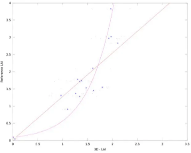
Figure 6 shows the reference LAIs with respect to the 3D-LAIs (field measurements). The 3D-LAI

under-C

A

estimated the reference one for reference LAIs above around 2. When plant grow, leaves recover each other and a saturation phenomenon is expected in the 3D-LAI compared with the reference LAI. The exponential regression (Fig. 6) showed a marginally higher correlation coefficient compared with the linear regression, respectively 0.93 and 0.89. However during the 2013 crop season, due to the prevailing meteorological conditions, the LAIs remained low compared with normal years. It is probable that for a more normal season, when the LAIs reach higher values (around 6), the saturation phenomenon would be more present and the exponential regression would perform clearly better than linear regression.

Neither the plant distribution along the sowing line nor their development are even. This means that when sampling the plants to measure the reference LAI, variations occur from one sample to another. The mean standard deviation of the four measurements coming from the different plot submitted to the same agronomic treatment was 0.23. The standard deviation for the estimation of the LAI based on individual 3D measurement was 0.39. This estimation error could be reduced by considering more samples. When the five images are taken into account, the standard deviation of the estimation drop to 0.17.

Fig. 6. Relation between 3D-LAI and reference LAI. 4. CONCLUSION

3D vision was tested to measure the leaf area index and the average leaf angle, two agronomic parameters useful to assess crop development. The accuracy and the precision of the proposed measurement were evaluated. When computed for an artificial know pattern or for a fixed spot in the field, the precision was around 0.1 for the LAI. Random errors in the evaluation of the camera-plant distance were at the origin of these variations. In the field, by using a regression between measured value and reference values, the LAI could be estimated with a standard deviation of 0.39. This was higher than the reference measurements. However, the precision could easily enhanced by acquiring a few images.

As 3D image acquisition is straightforward, while reference sampling were time consuming, 3D measures of the LAI could thus be more efficient.

5. REFERENCES

[1] Jonckheere, I., Fleck, S., Nackaerts, K., Muys, B., Coppin, P., Weiss, M., Baret, F.: Review of methods for in situ leaf area index determination. Part I. Theories, sensores and hemispherical photography. Agricultural and Forest Meteorology, 121:19-35, 2004.

[2] Bréda, N.: Ground_based measurements of leaf area index : a review of methods, instruments and current controversies. Journal of Experimental Botany, 54(392):2403-2417, 2003. [3] Aparicio, N., Villegas, D., Casadesús, J., Araus, J.L., Royo, C.:

Spectral vegetation indices as a non-destructive tool for determining durum wheat yield. Agron. J., 92:83–91, 2000. [4] Kirk, J., Andersen, J.H., Thomsen, A.G., Jørgensen, J.R.,

Jørgensen, R.N.: Estimation of leaf area index in cereal crops using red-green images. Biosystems Engineering, 104:308-317, 2009.

[5] Baret, F., de Solan, B., Lopez-Lozano, R., Kai Ma, Weiss, M.: GAI estimates of row crops from downward looking digital photos taken perpendicular to the row at 57.5° zenit angle : Theoretical considerations based on 3D architecture models and application to wheat crops. Agricultural and Forest Meteorology, 150:1393-1401, 2010.

[6] Dammer, K.-H., Wollny, J., Giebel, A.: Estimation of the Leaf Area Index in cereal crops for variable rate fungicide spraying. European Journal of Agronomy, 28:351-360, 2008.

[7] Andersen, H., J., Reng, L., Kirk, K.: Geometric plant properties by relaxed stereo vision using simulated annealing. Computers and electronics in agriculture, 49:219-232, 2005. [8] Bradski, G., Kaehler, A.: Learning OpenCV: Computer Vision

with the OpenCV Library. O'Reilly, Sebastopol (CA), pp 556, 2008.