Vibration Assessment of Ship Structures
Texte intégral
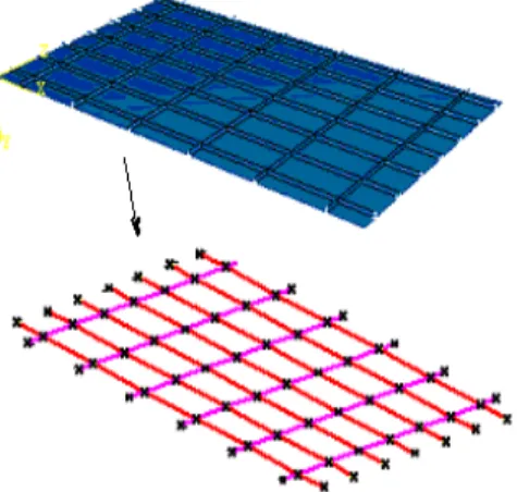
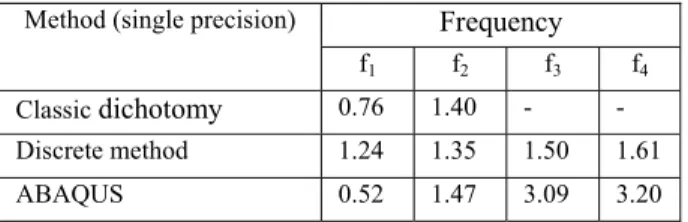
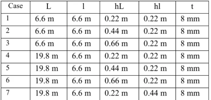
Figure


Documents relatifs
La distribution de la distance résiduelle du satellite cible et le nombre moyen de handover intersatellite durant un appel, lorsque plusieurs satellites peuvent être vus
86 تدعوو ايسايس ةقفصلا معد يف نيصلا تكراش امك ،ناريإ يف كلذب مايقلا نم لادب يناريلإا ربكأ تناك نادلبلا هذه نأ كلذ نم مهلأاو ،ةيندم ةيوون تاردقب
Singular manifolds of proteomic drivers to model the evolution of inflammatory bowel disease
(depending on the expression level of the protein and its rate of ubiquitylation). Tandem purification of a protein in denaturing conditions for the identification
De nos jours et chez les jeunes particulièrement, travailler n’est plus « qu’une façon d’obtenir un salaire ou de gagner sa vie, mais aussi un moyen pour se réaliser
nt hydroxyle en C3 figure [I.9.]. Elles sont les flavonoïdes les plus répandus dans le règne végétal, leur couleur varie du blanc au jaune, elles sont essentiellement
3.2 Des modèles de distribution d’abondance pour évaluer le paramètre « structure et fonction » Les relevés réalisés dans les hêtraies acidiphiles à houx (9120 ALP), les
The Compound Term Composition Algebra (CTCA) is an al- gebra with four algebraic operators, whose composition can be used to specify the meaningful (valid) compound terms
