HAL Id: inria-00537810
https://hal.inria.fr/inria-00537810
Submitted on 19 Nov 2010
HAL is a multi-disciplinary open access
archive for the deposit and dissemination of
sci-entific research documents, whether they are
pub-lished or not. The documents may come from
teaching and research institutions in France or
abroad, or from public or private research centers.
L’archive ouverte pluridisciplinaire HAL, est
destinée au dépôt et à la diffusion de documents
scientifiques de niveau recherche, publiés ou non,
émanant des établissements d’enseignement et de
recherche français ou étrangers, des laboratoires
publics ou privés.
A Certified Denotational Abstract Interpreter
David Cachera, David Pichardie
To cite this version:
David Cachera, David Pichardie. A Certified Denotational Abstract Interpreter. International
Con-ference on Interactive Theorem Proving (ITP), 2010, Edimburgh, United Kingdom. pp.9-24.
�inria-00537810�
A Certified Denotational Abstract Interpreter
⋆ (Proof Pearl)David Cachera1and David Pichardie2
1
IRISA / ENS Cachan (Bretagne), France 2
INRIA Rennes – Bretagne Atlantique, France
Abstract. Abstract Interpretation proposes advanced techniques for static analysis of programs that raise specific challenges for machine-checked soundness proofs. Most classical dataflow analysis techniques it-erate operators on lattices without infinite ascending chains. In contrast, abstract interpreters are looking for fixpoints in infinite lattices where widening and narrowing are used for accelerating the convergence. Smart iteration strategies are crucial when using such accelerating operators because they directly impact the precision of the analysis diagnostic. In this paper, we show how we manage to program and prove correct in Coqan abstract interpreter that uses iteration strategies based on pro-gram syntax. A key component of the formalization is the introduction of an intermediate semantics based on a generic least-fixpoint operator on complete lattices and allows us to decompose the soundness proof in an elegant manner.
1
Introduction
Static program analysis is a fully automatic technique for proving properties about the behaviour of a program without actually executing it. Static analy-sis is becoming an important part of modern software design, as it allows to screen code for potential bugs, security vulnerabilities or unwanted behaviours. A significant example is the state-of-the-art Astr´ee static analyser for C [7] which has proven some critical safety properties for the primary flight control software of the Airbus A340 fly-by-wire system. Taking note of such a success, the next question is: should we completely trust the analyser? In spite of the nice mathematical theory of program analysis and the solid algorithmic techniques available one problematic issue persists, viz., the gap between the analysis that is proved correct on paper and the analyser that actually runs on the machine. To eliminate this gap, it is possible to merge both the analyser implementation and the soundness proof into the same logic of a proof assistant. This gives raise to the notion of certified static analysis, i.e. an analysis whose implementation has been formally proved correct using a proof assistant.
There are three main kinds of potential failures in a static analyser. The first one is (un)soundness, i.e. when the analyser guarantees that a program is safe but it is not. The second one deals with termination, when the analyser loops for
some entries. The third one is the problem of precision: given a choice of value approximation, the analyser may not make optimal choices when approximating some operations. For instance, a sign analyser that approximates the multipli-cation of two strictly positive values by the property “to be positive” is sound be not optimal since the best sound property is “to be strictly positive”.3 Only
the first kind of failure is really critical. However, revealing the other bugs too late during a validation campaign may compromise the availability of the safety critical system that has to be validated in due time.
In this paper we focus on the two first classes of potential failures, that is we prove the semantic soundness of an abstract interpreter and addresses the termination problem for a challenging fixpoint iteration scheme. Most classical dataflow analysis techniques look for the least solution of dataflow (in)equation systems by computing the successive iterates of a function from a bottom el-ement, in a lattice without infinite ascending chains. When each equation is defined by means of monotone operators, such a computation always termi-nates on an optimal solution, i.e. the least element of the lattice that satisfies all (in)equations. In contrast, abstract intepreters are generally looking for fixpoints in infinite lattices, where widening and narrowing operators are used for ensur-ing and acceleratensur-ing the convergence. Smart iteration strategies are crucial when using such accelerating operators because they directly impact the precision of the analysis diagnostic.
This article shows how we manage to program and prove correct in Coq an abstract interpreter that uses iteration strategies based on program syntax. The purpose of the current paper is not to define widening/narrowing operators but rather use them with the right iteration strategy. We focus on a small impera-tive language and consider abstact interpreters that automatically infer sound invariants at each program point of a program.
Our main contribution is an elegant embedding of the Abstract Interpreta-tion (AI) proof methodology: as far as we know, this is the first time the slogan “my abstract interpreter is correct by construction” is turned into a precise machine-checked proof. A key component of the formalization is the introduc-tion of an intermediate semantics with respect to which the soundness of the analyser is easily proved (hence the term by construction). The most difficult part arises when formally linking this semantics with a standard one.
The paper is organized as follows. Section 2 introduces the problem of it-eration strategies for fixpoint approximation by widening/narrowing. Section 3 briefly presents the syntax and the standard semantics of our While language. Section 4 describes the lattice theory components that are necessary for the definition of the intermediate collecting semantics described in Section 5. Sec-tion 6 presents the abstract interpreter together with its modular architecture. Then, we conclude after a discussion of related work. Except in Section 2, all formal definitions in this paper are given in Coq syntax. We heavily rely on the new type classes features [17] in order to use concise overloaded notations that
3
This kind of “bug” is sometimes a feature in order to find a pragmatic balance between precision and algorithmic complexity.
should allow the reader to understand the formal definitions without much Coq knowledge.
2
Static Analysis with Convergence Acceleration by
Widening/Narrowing
In this section, we illustrate with a simple program example the static analysis techniques that we consider. The target language is a minimalistic imperative language whose syntax is given in Section 3. The program given on Figure 1a is the core of a two-dimensional array scan with two nested loops of indexes i
and j. To each program point pc in {1..5} a pair of two intervals Ipc and Jpc
is associated, each one corresponding to an over-approximation of the possible values of variablesiandjat point pc.
i = 0; j = 0; 1: while j < 10 { i = 0; 2: while i < 10 { i = i + 1; 3: }; j = j + 1; 4: }; 5:
(a) Program code
(I1, J1) = ([0; 0], [0; 0]) ⊔ (I4, J4) (I2, J2) = ([0; 0], J1∩[−∞; 9]) ⊔ (I3, J3) (I3, J3) = (incr♯(I2), J2) (I4, J4) = (I2∩[10; +∞], incr♯(J2)) (I5, J5) = (I1, J1∩[10; +∞]) (b) Analysis equations
Fig. 1: An example of interval analysis
The analysis is specified by mutually recursive equations relating the inter-vals to each other. Figure 1b lists the equations corresponding to our example. The domain of intervals is equipped with a special bottom element ⊥, and ab-stract operators like intersection (∩), convex union (⊔) or abab-stract incremen-tation (incr♯ defined by incr♯([a, b]) = [a + 1, b + 1] and extended naturally to infinite values). These equations can be summarized as X = F (X), where X denotes the vector (X1, X2, X3, X4, X5) and each Xi denotes a pair of intervals.
The components of F will be denoted by Fi, i∈ {1..5} in the rest of this section.
The set of intervals on integers forms a lattice ordered by inclusion, where the lub and glb operators are the convex union and intersection, respectively. Ideally, the result of the analysis should be the least fixpoint of the set of equations. However, the lattice of intervals is of infinite height, which generally prevents us from computing a solution in finite time with a simple Kleene iteration. For instance, ∅ ⊂ [0, 0] ⊂ [0, 1] ⊂ [0, 2] ⊂ · · · ⊂ [0, n] ⊂ . . . is an infinite increasing chain. Instead of computing a least fixpoint, we can accommodate ourselves with an over-approximation, keeping correction in mind, but losing optimality.
The solution proposed by P. and R. Cousot [6] consists in accelerating the ascending iteration, thus reaching a post-fixpoint, but not necessarily the least one. This is done by using a binary widening operator ▽, that extrapolates both of its arguments, and use an iteration of the following form: x0 = ⊥, xn+1 =
xn▽f(xn). Intuitively, at the n-th iteration, the n-th iterate of the function is
compared to the preceeding value, in order to conjecture some possible over-approximation of the limit of the iteration sequence. In the infinite chain above, we would like to replace interval [0, n] by [0, +∞] after a finite (preferably small) number of iterations. We would like for instance that [0, 1]▽[0, 2] = +∞.
When a post-fixpoint is reached, a new iteration starting from this point may give a better solution, closer to the least fixpoint. The same termination issues appear, and may be treated by the use of a narrowing operator ∆.
The equations of the analysis are thus augmented with a set W of program points where widenings or narrowings are performed. We now have to determine a strategy for computing a fixpoint, i.e. an oracle for choosing an equation during the following standard chaotic iteration.
– Start with X = (⊥, ⊥, ⊥, ⊥, ⊥).
– Repeat until a post-fixpoint is reached the following steps • Choose (oracle) a point pc,
• if pc is a widening/narrowing point, replace Xpc by Xpc▽Fpc(X)
other-wise by Xpc⊔ Fpc(X).
– Repeat until stabilization the following steps • Choose (oracle) a point pc,
• if pc is a widening/narrowing point, replace Xpc by Xpc∆Fpc(X)
other-wise by Xpc⊓ Fpc(X).
Several technical difficulties appear with iteration strategies. First, widen-ing/narrowing points must be placed in order to cover all equations dependency cycles, otherwise the iteration may not terminate. On the contrary, using too many points may decrease the precision of the final result. Secondly, the itera-tion strategy (oracle) has a direct impact on the precision of the result because of the non-monotone nature of widening/narrowing operators.
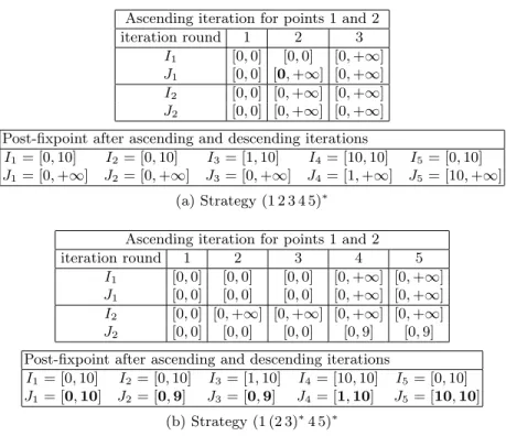
To illustrate these points, let us consider two strategies for our analysis ex-ample. Both strategies have widening/narrowing points at 1 and 2, the loop entries. The first one examines all equations in sequence with order 1 2 3 4 5 until stabilization. The second one has an inner iteration: it waits until the inner loop (2 3)∗ stabilizes before computing equations 4 and 5. Results are displayed in
Figure 2.
We give for each strategy the details of the ascending iteration with widening for points 1 and 2, and the final result after widening and narrowing iterations for all control points. This example shows the importance of choosing a good strategy: the second strategy which includes an “inner” iteration between points 2 and 3 yields a more precise result. This comes from the widenings performed at point 2: with strategy (1 2 3 4 5)∗ (Figure 2a), a widening is performed at the
second iteration round on both variablesiandj; as J2depends on J1computed
Ascending iteration for points 1 and 2 iteration round 1 2 3 I1 [0, 0] [0, 0] [0, +∞] J1 [0, 0] [0, +∞] [0, +∞] I2 [0, 0] [0, +∞] [0, +∞] J2 [0, 0] [0, +∞] [0, +∞] Post-fixpoint after ascending and descending iterations
I1 = [0, 10] I2 = [0, 10] I3= [1, 10] I4= [10, 10] I5= [0, 10] J1 = [0, +∞] J2 = [0, +∞] J3= [0, +∞] J4= [1, +∞] J5= [10, +∞]
(a) Strategy (1 2 3 4 5)∗ Ascending iteration for points 1 and 2 iteration round 1 2 3 4 5
I1 [0, 0] [0, 0] [0, 0] [0, +∞] [0, +∞] J1 [0, 0] [0, 0] [0, 0] [0, +∞] [0, +∞] I2 [0, 0] [0, +∞] [0, +∞] [0, +∞] [0, +∞] J2 [0, 0] [0, 0] [0, 0] [0, 9] [0, 9] Post-fixpoint after ascending and descending iterations
I1 = [0, 10] I2= [0, 10] I3= [1, 10] I4 = [10, 10] I5= [0, 10] J1 = [0, 10] J2= [0, 9] J3= [0, 9] J4 = [1, 10] J5= [10, 10]
(b) Strategy (1 (2 3)∗4 5)∗ Fig. 2: Example of iteration strategies
i; on the contrary, with strategy (1 (2 3)∗4 5)∗ (Figure 2b), the value of J 1is not
modified along the inner iteration (2 3)∗, so that J2is not “widened” too early.
Strategy (1 (2 3)∗4 5)∗is not taken at random: it exactly follows the syntactic
structure of the program, computing fixpoints as would a denotational semantics do. This is why we consider this kind of strategy in this paper.
3
Language Syntax and Operational Semantics
The analyser we formalize here is taken from an analysis previously designed by Cousot [5]. We consider a minimal While language whose concrete Coq syntax is given below. Programs are labelled4
with elements of typeword, which plays a special role in all our development. It is the type of Coq binary numbers with at most 32 bits and is hence inhabited with a finite number of objects. This property is crucial in order to ensure termination of fixpoint iteration on arrays indexed by keys of type word (cf. Section 6). A program is made from a main
instruction, an end label and a set of local variables. The syntax of instructions contains assignments of a variable by a numeric expression, conditionals, while loops.
4
Definition var := word. Definition pp := word.
Inductive op := Add | Sub | Mult. Inductive expr :=
Const (n:Z) | Unknown | Var (x:var) | Numop (o:op) (e1 e2:expr).
Inductive comp := Eq | Lt. Inductive test :=
| Numcomp (c:comp) (e1 e2:expr) | Not (t:test) | And (t1 t2:test) | Or (t1 t2:test).
Inductive instr :=
Assign (p:pp) (x:var) (e:expr) | Skip (p:pp)
| Assert (p:pp) (t:test) | If (p:pp) (t:test) (b1 b2:instr) | While (p:pp) (t:test) (b:instr) | Seq (i1:instr) (i2:instr).
Record program := { p_instr:instr; p_end: pp; vars: list var }.
We give to this language a straightforward small-step operational semantics. An environment maps variable names to numerical values. A configuration is either a final environment or an intermediate configuration. The operational se-mantics takes the form of a judgment(sos p k (i,ρ) s)that reads as follows: for a program pthere is a one-step transition between an intermediate
config-uration (i,ρ) (an instruction and an environment) towards configuration s.
Predicate(subst ρ1 x n ρ2)expresses that the environmentρ2 is the result of the substitution ofxbyninρ1. The elementkrecords the kind of transition
that is taken. It is a technical trick that will be used and explained later in Section 5. At last, we build the reflexive transitive closuresos_starofsos.
Definition env := var → Z.
Inductive config := Final (ρ:env) | Inter (i:instr) (ρ:env).
Inductive sos (p:program) : Kind → (instr*env) → config → Prop :=
| sos_assign : ∀ l x e n ρ1 ρ2,
sem_expr p ρ1 e n → subst ρ1 x n ρ2 → In x (vars p) → sos p (KAssign x e) (Assign l x e,ρ1) (Final ρ2) [...]
| sos_while_true : ∀ l t b ρ, sem_test p ρ t true →
sos p (KAssert t) (While l t b,ρ) (Inter (Seq b (While l t b)) ρ) | sos_while_false : ∀ l t b ρ,
sem_test p ρ t false →
sos p (KAssert (Not t)) (While l t b,ρ) (Final ρ) | sos_seq1 : ∀ k i1 i2 ρ ρ’,
sos p k (i1,ρ) (Final ρ’) →
sos p (KSeq1 i (first i2)) (Seq i1 i2,ρ) (Inter i2 ρ’) | sos_seq2 : ∀ k i1 i1’ i2 ρ ρ’,
sos p k (i1,ρ) (Inter i1’ ρ’) →
sos p (KSeq2 k) (Seq i1 i2,ρ) (Inter (Seq i1’ i2) ρ’).
Inductive sos_star (p:program) : (instr*env) → config → Prop :=
| sos_star0 : ∀ i ρ, sos_star p (i,ρ) (Inter i ρ)
| sos_star1 : ∀ k s1 s2, sos p k s1 s2 → sos_star p s1 s2 | sos_trans : ∀ k s1 i ρ s3,
The soundness theorem of the analyser is expressed in terms of labelled reach-able states in (pp * env). A special label p_end is attached to final
environ-ments. Functionfirstrecursively computes the left-most label of an instruction.
Inductive reachable_sos (p:program) : pp*env → Prop :=
| reachable_sos_intermediate : ∀ ρ0 i ρ, sos_star p (p_instr p,ρ0) (Inter i ρ) → reachable_sos p (first i,ρ)
| reachable_sos_final : ∀ ρ0 ρ,
sos_star p (p_instr p,ρ0) (Final ρ) → reachable_sos p (p_end p,ρ).
4
Lattice Theory Intermezzo
Abstract Interpretation heavily relies on lattice theory to formalize semantic notions and approximation of properties. In order to define the suitable interme-diate semantics on our While language in the next section, we need to define a least fixpoint operator that is defined on complete lattices. We then introduce several packed structures for equivalence relations, partial orders and complete lattices. We use here type classes that give elegant notations for defining Coq records with implicit arguments facilities. Coercions are also introduced in order to define(Equiv.t A)as subclass of(Poset.t A)(notation:>in the fieldeqof
the class typePoset.t) and view subset components of typesubset Aas
sim-ple predicates on A (command Coercion charact : subset >->Funclass).
Some parameters are given with curly braces ‘{...} in order to declare them
as implicit. All these features make the formal definition far more elegant and concise. For example, in the type declaration of the fieldjoin_bound, the term
subset Ahides an object (Poset.eq A porder) of type (Equiv.t A)which
is automatically taken from the field porder : Poset.t A of the class type CompleteLattice.tand the coercion between(Equiv.t A)and(Poset.t A).
We also introduce definitions for lattices (type class Lattice.t) with the
corresponding overloaded symbols ⊥, ⊤, ⊓, ⊔ but do not show them here, due to space constraints.
Module Equiv.
Class t (A:Type) : Type :=
{ eq : A → A → Prop;
refl : ∀ x, eq x x; sym : [...]; trans : [...] }.
End Equiv.
Notation "x == y" := (Equiv.eq x y) (at level 40). Module Poset.
Class t A : Type :=
{ eq :> Equiv.t A; order : A → A → Prop;
refl : [...]; antisym : [...]; trans : [...] }.
Notation "x ⊑ y" := (Poset.order x y) (at level 40). Class subset A {Equiv.t A} : Type := SubSet {
charact : A → Prop;
subset_comp_eq : ∀ x y:A, x==y → charact x → charact y}.
Coercion charact : subset >-> Funclass. Module CompleteLattice.
Class t (A:Type) : Type := {
porder :> Poset.t A; join : subset A → A;
join_bound : ∀x:A, ∀f:subset A, f x → x ⊑ join f;
join_lub : ∀f:subset A, ∀z, (∀ x:A, f x → x ⊑ z) → join f ⊑ z;}.
End CompleteLattice.
Several canonical structures can be defined for these types. They will be automatically introduced by the inference system when objects of these types will be wanted by the type checker.
Notation "’P’ A" := (A → Prop) (at level 10).
Instance PowerSetCL A : CompleteLattice.t (P A) := [...] Instance PointwiseCL A L {CompleteLattice.t L} :
CompleteLattice.t (A → L) := [...]
Monotone functions are defined with a dependent pair and a coercion.
Class monotone A {Poset.t A} B {Poset.t B} : Type := Mono {
mon_func : A → B;
mon_prop : ∀ a1 a2, a1 ⊑ a2 → (mon_func a1) ⊑ (mon_func a2)}.
Coercion mon_func : monotone >-> Funclass.
We finish this section with the classical Knaster-Tarski theorem.
Definition lfp ‘{CompleteLattice.t L} (f:monotone L L) : L :=
CompleteLattice.meet (PostFix f). Section KnasterTarski. Variable L : Type. Variable CL : CompleteLattice.t L. Variable f : monotone L L. Lemma lfp_fixpoint : f (lfp f) == lfp f. [...] Lemma lfp_least_fixpoint : ∀ x, f x == x → lfp f ⊑ x. [...] Lemma lfp_postfixpoint : f (lfp f) ⊑ lfp f. [...] Lemma lfp_least_postfixpoint : ∀x, f x ⊑ x → lfp f ⊑ x. [...] End KnasterTarski.
5
An Intermediate Collecting Semantics
We now reach the most technical part of our work. One specific feature of the AI methodology is to give program semantics and program static analyses the same
shape. To that purpose, a collecting semantics is used instead of the standard semantics. Its purpose is still to express the dynamic behaviour of programs but it takes a form closer to that of a static analysis, namely being expressed as a least fixpoint of an equation system. In this work, we want to certify an abstract interpreter that inductively follows the syntax of programs and iterates each loop until convergence. We will thus introduce a collecting semantics that follows the same strategy, but computes on concrete properties.
In all this section we fix a programprog:program. We first introduce three
semantic operators. Operatorassign is the strongest post-condition of the
as-signment of a variable by an expression. Operatorassertis the strongest
post-condition of a test. The collecting semantics binds each program point to a property over reachable environments so that the semantic domain for this se-mantics is pp →P (A). An element in this domain can be updated with the functionEsubst. Note that it is a weak update since we take the union with the previous value.
Definition assign (x:var) (e:expr) (E:P(env)) : P(env) :=
fun ρ => ∃ρ’, ∃n, E ρ’ ∧ sem_expr prog ρ’ e n ∧ subst ρ’ x n ρ.
Definition assert (t:test) (E:P(env)) : P(env) := fun ρ => E ρ ∧ sem_test prog ρ t true.
Definition Esubst ‘(f:pp → P(A)) (k:pp) (v:P(A)) : pp → P(A) := fun k’ => if pp_eq k’ k then (f k) ⊔ v else f k’.
Notation "f +[ x 7→ v ]" := (Esubst f x v) (at level 100).
The collecting semantics is then defined by induction on the program syntax. Function(Collect i l)computes for an instructioniand a labell, a mono-tone predicate transformer such that for each initial propertyEnv:P (env), all
states(l’,ρ)that are reachable by the execution ofifrom a state in Env,
sat-isfy(Collect i l Env l’ ρ) where l’is either a label in ior is equal to l.
The label l should represent the next label afteriin the whole program. The
monotony property of this predicate transformer returned by(Collect i l)is
crucial if want to be able to use the lfp operator of the previous section that
takes only monotone functions as argument. For each instruction, we hence build a term of the form(Mono F _)withF a function and_a “hole” for the proof
that ensures the monotony ofF. All these holes give rise to proof obligations that
are generated by theProgrammechanism and must be interactively discharged
after the definition ofCollect.
Program Fixpoint Collect (i:instr) (l:pp):
monotone (P(env)) (pp → P(env)) :=
match i with
| Skip p => Mono (fun Env => ⊥ +[p 7→ Env] +[l 7→ Env]) _ | Assign p x e =>
Mono (fun Env => ⊥ +[p 7→ Env] +[l 7→ assign x e Env]) _ | Assert p t =>
Mono (fun Env => ⊥ +[p 7→ Env] +[l 7→ assert t Env]) _ | If p t i1 i2 =>
Mono (fun Env =>
let C2 := Collect i2 l (assert (Not t) Env) in
(C1 ⊔ C2) +[p 7→ Env]) _ | While p t i =>
Mono (fun Env =>
let I:P(env) := lfp (iter Env (Collect i p) t p) in
(Collect i p (assert t I))
+[p 7→ I] +[l 7→ assert (Not t) I]) _ | Seq i1 i2 =>
Mono (fun Env => let C := (Collect i1 (first i2) Env) in C ⊔ (Collect i2 l (C (first i2)))) _
end.
TheWhile instruction is the most complex case. It requires to compute a
predicateI:P (env)that is a loop invariant bound to the labelp. It is the least
fixpoint of the monotone operatoriter defined below.
Program Definition iter (Env:P(env))
(F:monotone (P(env)) (pp → P(env)))
(t:test) (l:pp) : monotone (P(env)) (P(env)) := (Mono (fun X => Env ⊔ (F (assert t X) l)) _).
We hence compute the least fixpointIof the following equation: I == Env ⊔ (Collect i p (assert t I) p)
The invariant is the union of the initial environment (at the entry of the loop) and the result of the transformation of I by two predicate transformers:assert t
takes into account the entry in the loop, and the recursive call to(Collect i p)
collects all the reachable environments during the execution of the loop bodyi
and select those that are bound to the label pat the loop header.
Such a semantics is sometimes taken as standard in AI works but here, we precisely prove its relationship with the more standard semantics of Section 3. For that purpose, we establish the following theorem.
Theorem sos_star_implies_Collect : ∀ i1 ρ1 s2, sos_star prog (i1,ρ1) s2 →
match s2 with
| Inter i2 ρ2 => ∀l:pp, ∀Env:P(env),
Env ρ1 → Collect i1 l Env (first i2) ρ2 | Final ρ2 => ∀l:pp, ∀Env:P(env),
Env ρ1 → Collect i1 l Env l ρ2
end.
This theorem is proved by induction on the hypothesissos_star prog s1 s2.
The first case corresponds to s2=Inter i1 ρ1and is proved thanks using the fact thatCollectis extensive.
Lemma Collect_extensive : ∀ i, ∀ Env:P(env), ∀l,
Env ⊑ Collect i l Env (first i).
The second case corresponds tosos prog s1 s2. It is proved thanks to the
Lemma sos_implies_Collect : ∀ k i1 ρ1 s2, sos prog k (i1,ρ1) s2 →
match s2 with
| Inter i2 ρ2 => ∀l:pp, ∀Env:P(env),
Env ρ1 → Collect i1 l Env (first i2) ρ2 | Final ρ2 => ∀l:pp, ∀Env:P(env),
Env ρ1 → Collect i1 l Env l ρ2
end.
The last case corresponds to the existence of an intermediate state(i,ρ)such thatsos prog k (i1, ρ1) (Inter i ρ)andsos_star prog (i, ρ) s2and the induction hypothesis holds for (Collect i). In order to connect this
in-duction hypothesis with the goal that deals with (Collect i1), we prove the
following lemma.
Lemma sos_transfer_incl : ∀ k i1 ρ1 i2 ρ2, sos prog k (i1,ρ1) (Inter i2 ρ2) → ∀Env:P(env), ∀l_end,
Collect i2 l_end (transfer k Env) ⊑ Collect i1 l_end Env.
Here(transfer k)is a suitable predicate transformer such that the
follow-ing lemma holds.
Lemma sos_transfer : ∀ k i1 ρ1 s2, sos prog k (i1,ρ1) s2 →
match s2 with
| Inter i2 ρ2 => ∀Env:P(env), Env ρ1 → (transfer k Env) ρ2 | Final ρ2 => ∀Env:P(env), Env ρ1 → (transfer k Env) ρ2
end.
It is defined by the following recursive function using the informationk:Kind
that we have attached to each semantic rule in Section 3.
Fixpoint transfer (k:Kind) (Env:P(env)) : P(env) := match k with
| KAssign x e => assign x e Env | KSkip => Env
| KAssert t => assert t Env | KSeq1 i l => Collect i l Env l | KSeq2 k => transfer k Env
end.
This ends the proof of theorem sos_star_implies_Collect, from which we can easily deduce that each reachable state in the standard semantics is reachable with respect to the collecting semantics.
Definition reachable_collect (p:program) (s:pp*env) : Prop := let (k,env) := s in Collect p (p_instr p) (p_end p) (⊤) k env. Theorem reachable_sos_implies_reachable_collect :
6
A Certified Abstract Interpreter
We now design an abstract interpreter that, instead of executing a program on environment properties as the previous collecting semantics do, computes on an abstract domain with a lattice structure. Such a structure is modelled with a type classAbLattice.tthat packs the same standard components as inLattice.t
but also decidable tests for equality and partial order, and widening/narrowing operators. It is equipped with overloaded notations ⊑♯, ⊓♯, ⊔♯, ⊥♯. This abstract
lattice structure has been presented in an earlier paper [14]. The lattice signa-ture contains a well-foundedness proof obligation which ensures termination of a generic post-fixpoint iteration algorithm.
Definition approx_lfp : ∀ ‘{AbLattice.t t}, (t → t) → t := [...] Lemma approx_lfp_is_postfixpoint : ∀ ‘{AbLattice.t t} (f:t → t),
f (approx_lfp f) ⊑♯ (approx_lfp f).
A library is provided to build complex lattice objects with various functors for products, sums, lists and arrays [14]. Arrays are defined by means of binary trees whose keys are elements of typeword. The corresponding functorArrayLattice
given below relies on the finiteness of word to prove the convergence of the
pointwise widening/narrowing operators on arrays.
Instance ArrayLattice t {L:AbLattice.t t}: AbLattice.t (array t).
We connect concrete and abstract lattices with concretization functions that enjoy a monotony property together with a meet morphism property. This for-malization choice is motivated by our previous study of embedding AI framework in the constructive logic of Coq [13].
Module Gamma.
Class t a A {Lattice.t a} {AbLattice.t A} : Type := {
γ : A → a;
γ_monotone : ∀ N1 N2:A, N1 ⊑♯ N2 → γ N1 ⊑ γ N2; γ_meet_morph : ∀ N1 N2:A, γ N1 ⊓ γ N2 ⊑ γ (N1 ⊓♯ N2) }.
End Gamma.
Coercion Gamma.γ : Gamma.t >-> Funclass.
Using the new Coq type class feature we have extended our previous lattice library with concretization functors in order to build concretization operators in a modular fashion. We show below the signature of the array functor. This kind of construction was difficult with Coq modules that are not first class citizens, whereas it is often necessary to let concretizations depend on elements as programs.
Instance GammaFunc ‘{Gamma.t a A} : Gamma.t (word → a) (array A).
Our abstract interpreter is parameterized with respect to an abstraction of program environments given below. The structure encloses a concretization oper-ator mapping environment properties to an abstract lattice, two correct approx-imations of the predicate transformers Collect.assignand Collect.assert
Module AbEnv.
Class t ‘(L:AbLattice.t A) (p:program) : Type := {
gamma :> Gamma.t (P env) A; assign : var → expr → A → A; assign_correct : ∀ x e,
(Collect.assign p x e) ◦ gamma ⊑ gamma ◦ (assign x e); assert : test → A → A;
assert_correct : ∀ t,
(Collect.assert p t) ◦ gamma ⊑ gamma ◦ (assert t); top : A;
top_correct : ⊤ ⊑ gamma top }.
End AbEnv.
The abstract interpreter AbSem is then defined in a section where we fix a program and an abstraction of program environments. Its definition perfectly mimics the collecting semantics. We use the abstract counterpartF +[p 7→Env]♯
of the operatorEsubst that has been defined in Section 5. The main difference
is found for theWhile instruction where we don’t use a least fixpoint operator
but the generic post-fixpoint solver approx_lfp.
Section prog.
Variable (t : Type) (L : AbLattice.t t)
(prog : program) (Ab : AbEnv.t L prog).
Fixpoint AbSem (i:instr) (l:pp) : t → array t := match i with
| Skip p => fun Env => ⊥♯ +[p 7→ Env]♯ +[l 7→ Env]♯ | Assign p x e =>
fun Env => ⊥♯ +[p 7→ Env]♯ +[l 7→ Ab.assign Env x e]♯ | Assert p t =>
fun Env => ⊥♯ +[p 7→ Env]♯ +[l 7→ Ab.assert t Env]♯ | If p t i1 i2 => fun Env =>
let C1 := AbSem i1 l (Ab.assert t Env) in let C2 := AbSem i2 l (Ab.assert (Not t) Env) in
(C1 ⊔♯ C2) +[p 7→ Env]♯ | While p t i => fun Env =>
let I := approx_lfp (fun X => Env ⊔♯
(get (AbSem i p (Ab.assert t X)) p)) in (AbSem i p (Ab.assert t I)) +[p 7→ I]♯+[l 7→ Ab.assert (Not t) I]♯ | Seq i1 i2 => fun Env =>
let C := (AbSem i1 (first i2) Env) in
C ⊔♯ (AbSem i2 l (get C (first i2)))
end.
This abstract semantics is then proved correct with respect to the collecting semantics Collect and the canonical concretization operator on arrays. The
proof is particularly easy becauseCollect andAbSemshare the same shape.
Lemma AbSem_correct : ∀ i l_end Env,
Collect prog i l_end (Ab.γ Env) ⊑ γ (AbSem i l_end Env).
At last we define the program analyser and prove that it computes an over-approximation of the reachable states of a program. This a direct consequence of the previous lemma. Note that this final theorem deals with the standard operational semantics proposed in Section 3. The collecting semantics in only used as an intermediate step in the proof.
Definition analyse : array t :=
AbSem prog.(p_instr) prog.(p_end) (Ab.top).
Theorem analyse_correct : ∀ k env,
reachable_sos prog (k,env) → Ab.γ (get analyse k) env.
In order to instantiate the environment abstraction, we provide a functor that builds a non-relational abstraction from any numerical abstraction by binding a numerical abstraction to each program variable.
Instance EnvNotRelational ‘(NumAbstraction.t L) (p:program) :
AbEnv.t (ArrayLattice L) p.
Due to the lack of space, the typeNumAbstraction.tis not described in this
paper. We have instantiated it with interval, sign and congruence abstractions. The different instances of the analyser can be extracted to Ocaml code and run on program examples5
.
7
Related Work
The analyser we have formalized here is taken from lecture notes by Patrick Cousot [5, 4]. We follow only partly his methodology here. Like him, we rely on a collecting semantics which gives a suitable semantic counterpart to the abstract interpreter. This semantics requires elements of lattice theory that, as we have demonstrated, fit well in the Coq proof assistant. One first difference is that we don’t take this collecting semantics as standard but formally link it with a standard small-step semantics. A second difference concerns the proof technique. Cousot strives to manipulate Galois connections, which are the standard abstract interpretation constructs used for designing abstract semantics. Given a concrete lattice of program properties and an abstract lattice (on which the analyser effectively computes), a pair of operators (α, γ) is introduced such that α(P ) provides the best abstraction of a concrete property P , and γ(P♯) is the least
upper bound of the concrete properties that can be soundly approximated by the abstract element P♯. With such a framework it is possible to express the most
precise correct abstract operator f♯= α ◦ f ◦ γ for a concrete f . Patrick Cousot
in another set of lecture notes [5] performs a systematic derivation of abstract transfers functions from specifications of the form α◦f ◦γ. We did not follow this kind of symbolic manipulations here because they will require much proof effort: each manipulation of α requires to prove a property of optimal approximation.
5
This is only useful for tracking the third category of static analysis failures we have mentioned in the introduction of this paper.
Our abstract interpreter may appear as a toy example but it is often pre-sented [16] as the core of the Astr´eestatic analyser for C [7]. The same iter-ation strategy is used and the restrictions on the C language that are common in many critical embedded systems (no recursion, restricted use of pointers) al-low Astr´eeto concentrate mainly on While static analysis techniques. We are currently studying how we might formally link our current abstract interpreter with the formal semantics [3] of the CompCert project. This project is dedicated to the certification of a realistic optimizing C compiler and has so far [10] only be interested in data flow analyses without widening/narrowing techniques.
The While language has been the subject of several machine-checked se-mantics studies [8, 12, 2, 9] but few have studied the formalization of abstract interpretation techniques. A more recent approach in the field of semantics for-malization is the work of Benton et al. [1] which gives a Coq forfor-malization of cpos and of the denotational semantics of a simple functional language. A first attempt of a certified abstract interpreter with widening/narrowing iteration techniques has been proposed by Pichardie [13]. In this previous work, the anal-yser was directly generating an (in)equation system that was solved with a naive round-robin strategy as in Figure 2a. The soundness proof was performed with respect to an ad-hoc small-step semantics. Bertot [2] has formalized an abstract interpreter whose iteration strategy is similar to ours. His proof methodology dif-fers from the traditional AI approach since the analyser is proved correct with respect to a weakest-precondition calculus. The convergence technique is more ad hoc than the standard widening/narrowing approach we follow. We believe the inference capability of the abstract interpreters are similar but again, our approach follows more closely the AI methodology with generic interfaces for abstraction environments and lattice structures with widening/narrowing. We hence demonstrate that the Coq proof assistant is able to follow more closely the textbook approach.
8
Conclusion and Perspectives
We have presented a certified abstract interpreter for a While language which is able to automatically infer program invariants. We have in particular studied the syntax-directed iteration strategy that is used in the Astr´eetool. A similar interpreter had been proposed earlier [2] but our approach follows more closely the AI methodology. The key ingredient of the formalization is an intermedi-ate collecting semantics which is proved conservative with respect to a classical structural operational semantics [15].
The current work is a first step towards a global objective of putting in the Coqproof assistant most of the advanced static analysis techniques that are used in an analyser like Astr´ee. We could enhance it by function calls, that would be very easy to handle if we avoid recursion: as our abstract interpreter is denota-tional, i.e. is able to take any abstract property as input of a block and compute
a sound over-approximation of the states reachable from it. In this work we have computed an invariant for each program point but Astr´ee spares some com-putations keeping as few invariants as possible during iteration, and we should also consider that approach. These topics only concern the generic interpreter but we will have to combine this core interpreter with suitable abstract domains like octogons for floating-point arithmetic [11] or fine trace abstractions [16].
References
1. N. Benton, A. Kennedy, and C. Varming. Some domain theory and denotational semantics in Coq. In Proc. of TPHOLs ’09, volume 5674, pages 115–130. Springer-Verlag, 2009.
2. Y. Bertot. Structural abstract interpretation, a formal study in Coq. In Language
Engineering and Rigorous Software Development, International LerNet ALFA Summer School 2008, volume 5520 of LNCS, pages 153–194. Springer, 2009. 3. S. Blazy and X. Leroy. Mechanized semantics for the Clight subset of the C
language. J. Autom. Reasoning, 43(3):263–288, 2009.
4. P. Cousot, Visiting Professor at the MIT Aeronautics and Astronautics Depart-ment, Course 16.399: Abstract Interpretation.
5. P. Cousot. The calculational design of a generic abstract interpreter. In M. Broy and R. Steinbr¨uggen, editors, Calculational System Design. NATO ASI Series F. IOS Press, Amsterdam, 1999.
6. P. Cousot and R. Cousot. Abstract interpretation: a unified lattice model for static analysis of programs by construction or approximation of fixpoints. In Proc.
of POPL’77, pages 238–252. ACM Press, 1977.
7. P. Cousot, R. Cousot, J. Feret, L. Mauborgne, A. Min´e, D. Monniaux, and X. Ri-val. The ASTR´EE analyser. In Proc. of ESOP’05, pages 21–30. Springer LNCS vol. 3444, 2005.
8. M. J. C. Gordon. Mechanizing programming logics in higher-order logic. In Current
Trends in Hardware Verfication and Automatic Theorem Proving, pages 387–439. Springer, 1988.
9. X. Leroy, Mechanized semantics, with applications to program proof and compiler verification, lecture given at the 2009 Marktoberdorf summer school.
10. X. Leroy. Formal certification of a compiler back-end, or: programming a compiler with a proof assistant. In Proc. of POPL’06, pages 42–54. ACM Press, 2006. 11. A. Min´e. Relational abstract domains for the detection of floating-point run-time
errors. In Proc. of ESOP’04, volume 2986 of LNCS, pages 3–17. Springer, 2004. 12. T. Nipkow. Winskel is (almost) right: Towards a mechanized semantics textbook.
Formal Aspects of Computing, 10:171–186, 1998.
13. D. Pichardie. Interpr´etation abstraite en logique intuitionniste : extraction d’analyseurs Java certifi´es. PhD thesis, Universit´e Rennes 1, 2005. In french. 14. D. Pichardie. Building certified static analysers by modular construction of
well-founded lattices. In Proc. of FICS’08, volume 212 of ENTCS, pages 225–239, 2008.
15. G. D. Plotkin. A structural approach to operational semantics. Journal of Logic
and Algebraic Programming, 60-61:17–139, 2004.
16. X. Rival and L. Mauborgne. The trace partitioning abstract domain. ACM Trans.
Program. Lang. Syst., 29(5), 2007.
17. M. Sozeau and N. Oury. First-class type classes. In Proc. of TPHOLs 2008, volume 5170 of LNCS, pages 278–293. Springer, 2008.