HAL Id: hal-01824467
https://hal-imt.archives-ouvertes.fr/hal-01824467
Submitted on 27 Jun 2018
HAL is a multi-disciplinary open access
archive for the deposit and dissemination of
sci-entific research documents, whether they are
pub-lished or not. The documents may come from
teaching and research institutions in France or
abroad, or from public or private research centers.
L’archive ouverte pluridisciplinaire HAL, est
destinée au dépôt et à la diffusion de documents
scientifiques de niveau recherche, publiés ou non,
émanant des établissements d’enseignement et de
recherche français ou étrangers, des laboratoires
publics ou privés.
Bash Datalog: Answering Datalog Queries with Unix
Shell Commands
Thomas Rebele, Thomas Tanon, Fabian Suchanek
To cite this version:
Thomas Rebele, Thomas Tanon, Fabian Suchanek. Bash Datalog: Answering Datalog Queries with
Unix Shell Commands. ISWC, Oct 2018, Monterey, CA, United States.
�10.1007/978-3-030-00671-6_33�. �hal-01824467�
Bash Datalog: Answering Datalog Queries
with Unix Shell Commands
Thomas Rebele, Thomas Pellissier Tanon, and Fabian Suchanek
Telecom ParisTech, Paris, France
Abstract. Dealing with large tabular datasets often requires extensive preprocessing. This preprocessing happens only once, so that loading and indexing the data in a database or triple store may be an overkill. In this paper, we present an approach that allows preprocessing large tabular data in Datalog – without indexing the data. The Datalog query is trans-lated to Unix Bash and can be executed in a shell. Our experiments show that, for the use case of data preprocessing, our approach is competitive with state-of-the-art systems in terms of scalability and speed, while at the same time requiring only a Bash shell, and a Unix-compatible oper-ating system.
1
Introduction
Motivation. Many data analytics tasks work on tabular data. Such data can take the form of relational tables or TAB-separated files. Even RDF knowledge bases can be seen abstractly as tabular data of a subject, a predicate, an object, and an optional graph. Quite often, such data has to be preprocessed before the analysis can be made. We focus here on preprocessing in the form of select-project-join-union operations with recursion – removing superfluous columns, selecting rows of interest, recursively finding all instances of a class, etc. The defining characteristic of such a preprocessing step is that it is executed only once on the data in order to constitute the dataset of interest for the later analysis. In this article, we focus on one-time preprocessing.
Databases or triple stores can obviously help. However, loading large amounts of data into these systems may take hours or even days (Wikidata [35], e.g., con-tains 267GB of data). Another possibility is to use systems such as DLV [20] and RDFox [24], which work directly on the data. However, these systems load the data into memory. While this works well for small datasets, it does not work for larger ones (as we show in our experiments). Large-scale data processing systems such as BigDataLog [31], Flink [7], Dryad [17], or NoDB [4] can help. However, these require the installation of particular software, the knowledge of particular programming languages, or even a particular distributed infrastruc-ture. Installing and getting to run such systems can take several hours. The user may not have the necessary knowledge and infrastructure to do this (think of a researcher in the Digital Humanities who wants to preprocess a file of census data; or of an engineer in a start-up who has to quickly join log files on a common column; or of a student who wants to extract a subgraph of Wikidata).
Our Proposal. In this paper, we propose a method to preprocess tabular data files without installing any particular software. We propose to express the prepro-cessing steps in Datalog [2]. For example, assume that there is a file facts.tsv that contains RDF facts in the form of TAB-separated subject-predicate-object triples. Assume that we want to recursively extract all places located in the United States. The Datalog program in our dialect would be:
fact(X, R, Y) :∼ cat facts.tsv
locatedIn(X, Y) :- fact(X, "locatedIn", Y) .
locatedIn(X, Y) :- locatedIn(X, Z), fact(Z, "locatedIn", Y) . main(X) :- locatedIn(X, "USA") .
The program prints the file facts.tsv into a predicate fact. The following two lines are the recursive definition of the locatedIn predicate. The main predicate is a predefined predicate that acts as the query. Our rationale for choosing Dat-alog is that it is a particularly simple language, which has just a single syntactic construction, and no reserved keywords. Yet, Datalog is expressive enough to deal with joins, unions, projections, selections, negation, and recursivity. In par-ticular, it can deal with n-ary tables (n > 2). However, if the user deals primarily with RDF data, our approach can also be used with N-Triples files as the A-Box, a subset of OWL 2 RL [23] as the T-Box, and SPARQL [16] for the query.
To execute the Datalog program, we propose to compile it automatically to Unix Bash Shell commands. We offer a Web page to this end: https://www. thomasrebele.org/projects/bashlog. The user can just enter the Datalog program, and click a button to obtain the following Bash code (simplified):
awk ’$2 == "locatedIn" {print $1 "\t" $3}’ facts.tsv > sc.tmp awk ’$2 == "USA" {print $0}’ sc.tmp | tee full.tmp > delta.tmp while
join sc.tmp delta.tmp | comm -23 - full.tmp > new.tmp mv new.tmp delta.tmp
sort -m -o full.tmp full.tmp delta.tmp [ -s delta.tmp ];
do continue; done cat full.tmp
The Bash code can be copy-pasted into a Unix Shell and run. Such a solution has several advantages. First, it does not require any software installation. It just requires a visit to a Web site. The resulting Bash code runs on any Unix-compatible system out of the box. Second, the Bash shell has been around for several decades, and the commands are not just tried and tested, but actually continuously developed. Modern implementations of the sort command, e.g., can split the input into several portions that fit into memory, and sort them individually. Finally, the Bash shell allows executing several processes in parallel, and their communication is managed by the operating system.
Contribution. We prose to compile a Datalog program automatically into Bash commands. Our method optimizes the Datalog program with relational algebra
optimization techniques, re-uses previously computed intermediate results, and produces a highly parallelized Shell script. For this purpose, our method employs pipes and process substitution. Our experiments on a variety of datasets and preprocessing tasks show that this method is competitive in terms of runtime with state-of-the-art database systems, Datalog engines, and triple stores.
We start with a discussion of related work in Section 2. Section 3 introduces preliminaries. Section 4 presents our approach, and Section 5 evaluates it.
2
Related Work
Data Processing Systems. Relational Databases such as Oracle, IBM DB2, Postgres, MySQL, MonetDB [5] and NoDB [4] can handle tabular data of ar-bitrary form, while the triple stores such as OpenLink Virtuoso [11], Stardog, and Jena [8] target RDF data. HDT [13] is a binary format for RDF, which can be used with Jena. RDFSlice (and its latest release Torpedo) [22] can pre-process RDF datasets. Reasoners such as Pellet [25], HermiT [30], RACER [15], Fact++ [33] and Jena [8] can perform OWL reasoning on RDF data. Datalog systems such as DLV [20], Myria [36], BigDatalog [31], DatalogRA [27], RD-Fox [24] and others [29,6,37,18] can efficiently evaluate Datalog queries on large data. Distributed Data Processing systems such as Dryad [17], Apache Tez [28], SCOPE [39], Impala [12], Apache Spark [38], and Apache Flink [7] provide ad-vanced features such as support for SQL or streams.
All of these systems can be used for preprocessing data. However, the vast majority of these systems require the installation of software. The parallelized systems also require a distributed infrastructure. Our approach, in contrast, requires none of these. It just requires a visit to a Web page. The Bash script that we produce runs in a common shell console without any further prerequisites. Interestingly, our approach still delivers comparable performance to the state of the art, as we shall see in the experiments.
Only very few systems do not require a software installation beyond down-loading a file (e.g., RDFSlice [22], Stardog, and DLV [20]). Yet, as we shall see in the experiments, these systems do not scale well to large datasets.
Other Work. Linked Data Fragments [34] aim to strike a balance between downloading an RDF data dump and querying it on a server. The method thus addresses a slightly different problem from ours. NoSQL Databases such as Cas-sandra, HBase, and Google’s BigTable [9] target non-tabular data. Our method, in contrast, aims at tabular data.
3
Preliminaries
Datalog. A Datalog rule with negation [1,2] takes the form H :— B1, . . . , Bn, ¬N1, . . . , ¬Nm.
Here, H is the head atom, B1, ..., Bnare the positive body atoms, and N1, ..., Nm
a relation name and x1, ..., xk ∈ V ∪ C, where V is a set of variables and C is
a set of constants. Intuitively, such a rule says that H holds if B1, ..., Bn and
none of the N1, ..., Nmholds. We consider only safe rules, i.e., each variable in
the head or in a negated atom must also appear in a positive body atom. A Datalog program is a set of Datalog rules. A set M of atoms is a model of a program P , if the following holds: M contains an atom a iff P contains a rule H :— B1, ..., Bn, ¬N1, . . . , ¬Nm, such that there exists a substitution σ : V → C
with σ(Bi) ∈ M for i ∈ {1, ..., n} and σ(Ni) 6∈ M for i ∈ {1, ..., m} and a = σ(H).
We consider only stratified Datalog programs [1,2], which entails that there exists a unique minimal model.
OWL RL [23] is a subset of the OWL ontology language. Since every OWL RL ontology can be translated to Datalog [24], we deal with Datalog as the more general case in all of the following.
Relational Algebra. Relational algebra [10,2] provides the semantics of rela-tional database operations on tables. For our purposes, we use the unnamed relational algebra with the operators select σ, project π, join on, anti-join ., and union ∪ (see [26] for their definitions). We also use the least fixed point operator (LFP) [3]. For a function f from a table to a table, LF P (f ) is the least fix point of f for the ⊆ relation. With this, our algebra has the same expressivity as safe stratified Datalog programs [2].
Example 2 (Relational Algebra): The following expression computes the transitive closure of a two-column table subclass:
LF P (λx : subclass ∪ π1,4(x on2=1x))
LFP computes the least fix point of a function. Here, the function is given by a lambda expression. To compute the least fix point, we execute the λ-function first with the empty table, x = ∅. Then the function returns the subclass table. Then we execute the function again on this result. This time, the function will join subclass with itself, project the resulting 3-column table on the first and last 3-column, and add in the original subclass table. We repeat this process until no more changes occur.
Unix. Unix is a family of multitasking computer operating systems, which are widely used on servers, smartphones, and desktop computers. One of the char-acteristics of Unix is that “Everything is a file”, which means that files, pipes, the standard output, the standard input, and other resources can all be seen as streams of bytes. Here, we are interested only in TAB-separated byte streams, i.e., streams that consist of several rows (sequences of bytes separated by a new-line character), which each consist of the same number of columns (sequences of bytes separated by a tabulator character).
The Bourne-again shell (Bash) is a command-line interface for Unix-like op-erating systems. A Bash command is either a built-in keyword, or a small pro-gram. We will only use commands of the POSIX standard. One of them is the awk command, which we use as follows:
This command executes the program p on the byte stream b, using the TAB as a separator for b. We will discuss different programs p later in this paper. Pipes. When a command is executed, it becomes a process. Two processes can communicate through a pipe, i.e., a byte stream that is filled by one process, and read by the other one. If the producing process is faster than the receiving one, the pipe buffers the stream, or blocks the producing process if necessary. In Bash, a pipe between process p1 and process p2 pipes can be constructed by
stating p1 | p2. A pipe can also be constructed “on the fly” by a so-called
process substitution, as follows: p1 <( p2 ). This construction pipes the output
of p2into the first argument of p1.
4
Approach
4.1 Our Datalog Dialect
In our Datalog dialect, predicates are alphanumerical strings that start with a lowercase character. Variables start with an uppercase letter. Constants are strings enclosed by double quotes. Constants may not contain quotation marks, TAB characters, or newline characters. For our purposes, the Datalog program has to refer to files or byte streams of data. For this reason, we introduce an additional type of rules, which we call command rules. A command rule takes the following form:
p(x1, ..., xn) :∼ c
Here, p is a predicate, x1, ..., xnare variables, and c is a Bash command.
Semanti-cally, this rule means that executing c produces a TAB-separated byte stream of n columns, which will be referred to by the predicate p in the Datalog program. In the simplest case, the command c just prints a file, as in cat facts.tsv. However, the command can also be any other Bash command, such as ls -1.
Our goal is to compute a certain output with the Datalog program. This output is designated by the distinguished head predicate main. An answer of the program is a grounded variant of the head atom of this rule that appears in the minimal model of the program. See again Figure 1 for an example of a Datalog program in our dialect. Our dialect is a generalization of standard Datalog, so that a normal Datalog program can be run directly in our system.
Our approach can also work in “RDF mode”. In that mode, the input consists of an OWL 2 RL [23] ontology, a SPARQL [16] query, and an N-Triples file F . We build a main predicate for the SPARQL query, and we use a small AWK program that converts F into a TAB-separated byte stream (see our technical report [26] for details). Much like in RDFox [24], we convert the OWL ontology into Datalog rules (see again [26]). For now, we support only a subset of OWL 2 RL: Like RDFox [24], we assume that all classes and properties axioms are provided by the ontology and will not be queried by the SPARQL query. We also do not yet support OWL axioms related to literals. Our SPARQL implementation supports basics graph patterns, property paths without negations, OPTIONAL, UNION and MINUS.
Algorithm 1: Translation from Datalog to relational algebra
1 fn mapPred (p, cache, P ) is 2 if p ∈ cache then 3 return xp
4 plan ← ∅; newCache ← cache ∪ {p} 5 foreach rule p(H1, ..., Hnh) :— r1(X 1 1, ..., Xn11), ..., rn(X n 1, ..., Xnnn), ¬q1(Y11, ..., Ym11), ..., ¬qm(Y m 1 , ..., Ymmm) in P do 6 bodyPlan ← {()} 7 foreach ri(X1i, . . . , Xnii) do
8 atomPlan ← mapPred(ri, newCache, P )
9 foreach (Xji, X i k) | X i j= X i k, j 6= k do 10 atomPlan ← σXi j=Xki(atomPlan)
11 bodyPlan ← bodyPlan on atomPlan 12 foreach ¬qi(Y1i, . . . , Ymii) do 13 atomPlan ← mapPred(qi, ∅, P ) 14 foreach (Yji, Y i k) | Y i j = Y i k, j 6= k do 15 atomPlan ← σYi j=Yki(atomPlan)
16 bodyPlan ← bodyPlan . atomPlan 17 plan ← plan ∪ πH1,...,Hnh(bodyPlan)
18 foreach rule p(H1, . . . , Hnh) :∼c in P do
19 plan ← plan ∪ πH1,...,Hnh(c)
20 return LF P (λxp: plan)
4.2 Loading Datalog
Next, we build a relational algebra expression for the main predicate of the Dat-alog program. Algorithm 1 takes as input a predicate p, a cache, and a DatDat-alog program P . The method is initially called with p=main, cache=∅, and the Dat-alog program that we want to translate. The cache stores already computed relational algebra plans. Our algorithm first checks whether p appears in the cache. In that case, p is currently being computed in a previous recursive call of the method, and the algorithm returns a variable x indexed by p. This is the variable for which we compute the least fix point.
Then, the algorithm traverses all rules with p in the head. For every rule ph(H1, . . . , Hnh) :— r1(X 1 1, . . . , X 1 n1), . . . , rn(X n 1, . . . , X n nn), ¬q1(Y 1 1, . . . , Y 1 m1), . . . , ¬qm(Y1m, . . . , Y m
mm), the algorithm recursively retrieves the plan for the ri and the qj. It then adds a nested σj=k if there are j, k such that Xji= X
i k, and
Yi
j = Yki respectively. Then it combines these expressions pair-wise from left to
right by adding the relevant join constraints between the ri. It also adds the
antijoin constraints between the results of the combinations of the left elements and the qj. Finally, it puts the resulting formula into a project-node that extracts
the relevant columns.
The implementation of the algorithm builds a directed acyclic graph (DAG) instead of a tree. When the function mapPred is called with the same arguments
as in a previous call, it returns the result of the previous call. This implemen-tation allows us to re-use the same sub-plan multiple times in the final query plan, thereby reducing its size. The technique will also allow the Bash programs to re-use results that have already been computed.
Example 3 (Datalog Translation): Assume that there is a two-column TAB-separated file subclass.tsv, which contains each class with its subclasses. Consider the following Datalog program P :
(1) directSubclass(x,y) :∼ cat subclass.tsv (2) main(x,y) :- directSubclass(x,y).
(3) main(x,z) :- directSubclass(x,y), main(y,z).
We call mapPred(main, ∅, P ). Our algorithm will go through all rules with the head predicate main. These are Rule 2 and Rule 3. For Rule 2, the algorithm will recursively call mapPred(directSubclass, {main}, P ). This will return LF P (λxdirectSubclass : ∅ ∪ [cat subclass.tsv]). Since
the lambda-expression does not contain the variable xdirectSubclass,
this is equivalent to [cat subclass.tsv]. For Rule 3, we call mapPred(directSubclass, {main}, P ), which returns [cat subclass.tsv] just like before. Then we call mapPred(main, {main}, P ), which re-turns xmain because main is in the cache. Thus, Rule 3 yields π1,4([cat subclass.tsv] on2=1xmain)). Finally, the algorithm constructs
LF P (λxmain: [cat subclass.tsv] ∪
π1,4([cat subclass.tsv] on2=1xmain))
4.3 Producing Bash Commands
The previous step has translated the input Datalog program to a relational algebra expression. Now, we translate this expression to a Bash command by the function b, which is defined as follows:
b([c]) = c
An expression of the form [c] is already a Bash command, and hence we can return directly c.
b(e1∪ ... ∪ en)
We translate a union into a sort command that removes duplicates: sort -u <(b(e1)) ... <(b(en))
b(e1onx=ye2)
A join of two expressions e1and e2on a single variable at position x and y,
respectively, gives rise to the command join -t$'\t' -1x -2y
<(sort -t$'\t' -kx <(b(e1)))
<(sort -t$'\t' -ky <(b(e2)))
This command sorts the byte streams of b(e1) and b(e2), and then joins them
b(e1onx=y,...e2)
The Bash join command can perform the join on only one column. If we want to join on several columns, we have to add a new column to each of the byte streams. This new column concatenates the join columns into a single column. This can be achieved with the following AWK program, which we run on both b(e1) and b(e2):
{ print $0 FS $j1 s $j2 s ... s $jn }
Here, the indices j1, ..., jn are the positions of the join columns in the input
byte stream, and s is a special separation character (we use ASCII character 2, but any other one can be used as well). Once we have done this with both byte streams, we can join them on this new column as described above. This join will also remove the additional column.
b(e1.xe2)
Just as a regular join, an antijoin becomes a join command. We use the parameter -v1, so that the command outputs only those tuples emerging from e1than cannot be joined with those from e2. We deal with antijoins on
multiple columns in the same way as with multicolumn joins. b(πi1,...in(e))
A projection becomes the following AWK program, which extracts the given columns from the input byte stream b(e):
{ print $i1 FS ... FS $in }
b(πi:a(e))
A constant introduction becomes the following AWK program, which pro-duces a TAB-separated byte stream that inserts the constant in column i of the input byte stream b(e):
{ print $1 FS ... $(i-1) FS a FS $i FS ... $n} b(σi=v(e))
A selection node gives rise to the following AWK program, which selects the corresponding rows from the input byte stream b(e):
$i=="v" { print $0 }
This command can be generalized easily to a selection on several columns. Several of these translations produce process substitutions. In such cases, Bash starts the parent process and the inner process in parallel. The parent process will block while it cannot read from the inner processes. Thus, only the innermost processes run in the beginning. Every process is run asynchronously as soon as input and CPU capacity is available. Thus, our Bash program is not subject to the forced synchronization that appears in Map-Reduce systems.
4.4 Recursion
We have just defined the function b that translates a relational algebra expression to a Bash command. We will now see how to define b for the case of recursion. A node LF P (f ) becomes
echo -n > delta.tmp; echo -n > full.tmp while
sort b(f (delta.tmp)) | comm -23 - full.tmp > new.tmp; mv new.tmp delta.tmp;
sort -u -m -o full.tmp full.tmp <(sort delta.tmp); [ -s delta.tmp ];
do continue; done cat full.tmp
This code uses 3 temporary files to compute the least fix point of f : full.tmp contains all facts inferred until the current iteration. delta.tmp contains newly added facts of an iteration. new.tmp is used as swap file. The code first creates delta.tmp and full.tmp as empty files. It then runs f on the delta file. The comm command compares the sorted outcome of f to the (initially empty) file full.tmp, and writes the new lines to the file new.tmp. This file is then renamed to delta.tmp. This procedure updates the file delta.tmp to contain the newly added facts. The comm command cannot write directly to delta.tmp, because this file also serves as input to the command produced by b(f (delta.tmp)).
The following sort command merges the new lines into full.tmp, and writes the output to full.tmp (unlike the comm command, the sort command can write to a file that also serves as input). Now, all facts generated in this iteration have been added to full.tmp. The [...] part of the code lets the loop run while the file delta.tmp is not empty, i.e., while new lines are still being added. If no new lines were added, the code quits the loop, and prints all facts. Note that, due to the monotonicity of our relational algebra operators, and due to the stratification of our programs, we can afford to run f only on the newly added lines.
4.5 Materialization
Materialization nodes. To avoid re-computing a relational algebra expres-sion that has already been computed, we introduce a new type of operator
mkfifo lock_t ( b(m) > t
mv lock_t done_t cat done_t & exec 3> done_t exec 3>&-) &
by→t(p)
rm t to the algebra, the materialization node. A
mate-rialization node £(m,(λy : p)) has two sub-plans: m is the plan that is used multiple times, and that we will materialize. Function (λy : p) is the main plan that uses the materialized plan. Variable y replaces all occurrences of m in the original plan (see [26] for details).
The translation to Bash is shown on the right. b is the Bash translation function defined in Sec-tion 4.3. t is a temporary file name. The code first creates a named pipe called lock t. Commands that use t have to wait until b(m) finishes. We
en-sure this by making these commands read from lock t. Since this pipe contains no data, the commands block. When b(m) finishes, the two exec commands close
the named pipe, thus unblocking the commands that need t. There can be a rare race condition: b(m) may finish before any process that listens on the pipe was started. In that case, the two exec commands will try to close a pipe that has no listeners. In such cases, the exec command will block. We solve this problem by reading from the pipe with a cat command that runs in the background. This way, the pipe has at least one listener, and the exec commands will close the pipe. This, however, brings a second problem: If the processes that listen on the pipe were still not started, they will try to listen to a closed pipe. To avoid this problem, we rename the pipe from lock t to done t. Such a renaming does not affect any processes that already listen on the pipe, but it will prevent any new processes from listening on the pipe under the old name.
by→t extends b as follows: by→t(y) generates the bash code cat t, and plan
nodes pi that have an immediate descendant t generate the bash code
cat lock t 2> /dev/null ; b(pi)
As explained above, the cat command blocks the execution until t is mate-rialized. The part “2> /dev/null” removes the error message in case cat is executed when the pipe was already renamed.
4.6 Optimization
Relational Algebra Optimizations. We apply the usual optimizations on our relational algebra expressions: we push selection nodes as close to the source as possible; we merge unions; we merge projects; we apply a simple join re-ordering. Additionally, we remove an occurence of a LFP variable, if it cannot contribute new facts; we remove LFP when there is no recursion; and we extract from an LFP node the non-recursive part of the inner plan (so that it is computed only once at the beginning of the fixed point computation). We also optimize fix point computations in the same way as in the semi-naive Datalog evaluation [2] (see again [26] for details).
Bash Optimizations. We collect different AWK commands that select or project on the same file into a single AWK command. This command runs only once through the file, and writes out all selections and projections into several files, one for each original AWK command. We replace multiple comparisons with constants on the same columns by a hash table lookup. We detect nested sort commands, and remove redundant ones. We run sort -u on the final output to make all results unique. We estimate the number of concurrently running sort commands, and assign each of them an equal amount of memory, if the buffer size parameter is available. Finally, we force all commands to use the same character set and sort order by adding the command export LC ALL=C to our program.
5
Experiments
We ran our method on several datasets, and compared it to several competitors. All experiments were run on a laptop with Ubuntu 16.04, an Intel Core
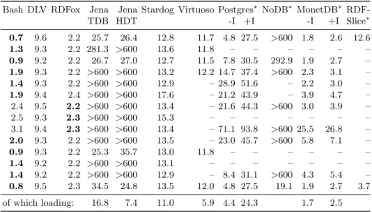
i7-Bash DLV RDFox Jena Jena Stardog Virtuoso Postgres∗ NoDB∗ MonetDB∗ RDF-TDB HDT -I +I -I +I Slice∗ 0.7 9.6 2.2 25.7 26.4 12.8 11.7 4.8 27.5 >600 1.8 2.6 12.6 1.3 9.3 2.2 281.3 >600 13.6 11.8 – – – – – – 0.9 9.2 2.2 26.7 27.0 12.7 11.5 7.8 30.5 292.9 1.9 2.7 – 1.9 9.3 2.2 >600 >600 13.2 12.2 14.7 37.4 >600 2.3 3.1 – 1.4 9.3 2.2 >600 >600 12.9 – 28.9 51.6 – 2.2 3.0 – 1.9 9.4 2.4 >600 >600 17.6 – 21.2 43.9 – 3.9 4.7 – 2.4 9.5 2.2 >600 >600 13.4 – 21.6 44.3 >600 3.0 3.9 – 2.5 9.3 2.3 >600 >600 15.3 – – – – – – – 3.1 9.4 2.3 >600 >600 13.4 – 71.1 93.8 >600 25.5 26.8 – 2.0 9.3 2.2 >600 >600 13.5 – 23.0 45.7 >600 5.8 7.1 – 0.9 9.3 2.2 25.3 35.7 13.0 11.8 – – – – – – 1.4 9.2 2.2 >600 >600 13.1 – – – – – – – 1.4 9.2 2.2 >600 >600 12.9 – 8.4 31.1 >600 4.3 5.4 – 0.8 9.5 2.3 34.5 24.8 13.5 12.0 4.8 27.5 19.1 1.9 2.7 3.7 of which loading: 16.8 7.4 11.0 5.9 4.4 24.3 1.7 2.5
Table 1. Runtime for the 14 LUBM queries with 10 universities (140 MB), in seconds.
∗
= no support for querying with a T-Box. We folded the T-Box into the query. +/-I = with/without indexes. A dash means that the query is not supported.
4610M 3.00 GHz CPU, 16 GB of memory, and 3.8 TB of disk space. We used GNU coreutils 8.25 for POSIX commands, and mawk 1.3.3 for AWK.
We emphasize that our goal is not to be faster than each and every system that currently exists. For this, the corpus of related work is simply too large (see Section 2). This is also not the purpose of Bash Datalog. The purpose of Bash Datalog is to provide a preprocessing tool that runs without installing any additional software besides a Bash shell. This is an advantage that no competing approach offers. Our experiments then serve mainly to show that our approach is generally comparable in terms of scalability with the state of the art.
5.1 Lehigh University Benchmark
Setting. The Lehigh University Benchmark (LUBM) [14] is a standard dataset for Semantic Web repositories, which models universities. It is parameterized by the number of universities, and hence its size can be varied. LUBM comes with 14 queries, which are expressed in SPARQL. We compare our approach to Stardog1, Virtuoso [11], RDFSlice [22], Jena [8], and Jena with the binary triple
format HDT [13]. For RDFox [24] and DLV [20], we translated the queries to Datalog in the same way that we translate the queries to Datalog for our own system (Section 4.2). For NoDB [4], Postgres2, and MonetDB [5], we translated
the queries to SQL. For this purpose, we used the relational algebra expression computed in Algorithm 1, together with the relational algebra optimizations
1
https://www.stardog.com/, v. 5.2.0
2
of Section 4.6. In this way, the T-Box of the LUBM queries is folded into the SQL query. Not all systems support all types of queries. MonetDB does not support recursive SQL queries. Postgres supports only certain types of recursive queries [26]. The same applies to NoDB. Virtuoso currently does not support intersections. RDFSlice aims at the slightly different problem of RDF-Slicing. It supports only a specific type of join. Also, it does not support recursion.
We ran every competitor on all queries that it supports, and averaged the runtime over 3 runs. Since most systems finished in a matter of seconds, we aborted systems that took longer than 10 minutes.
LUBM10. Table 1 shows the runtimes of all queries on LUBM with 10 universi-ties. The runtimes include the loading and indexing times. For systems where we could determine these times explicitly, we noted them in the last row of the table. Among the 4 triple stores (Jena+TDB, Jena+HDT, Stardog, and Virtuoso), only Stardog can finish on all queries in less than 10 minutes. RDFSlice can answer only 2 queries, and runs a bit faster than Stardog. The 5 database competitors (Postgres, NoDB, and MonetDB – with and without indexes) are generally faster. Among these, MonetDB is much faster than Postgres and NoDB. Postgres and MonetDB are fastest without indexes, which is to be expected when running the query only once. The best performing systems are the 3 Datalog systems (Bash Datalog, DLV, and RDFox). RDFox shines with a very short and nearly constant time for all queries. We suspect that this time is given by the loading time of the data, and that it dominates the answer computation time. Nevertheless, Bash Datalog is faster than RDFox on nearly all queries on LUBM 10.
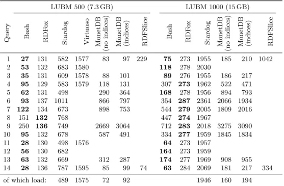
LUBM 500 (7.3 GB) LUBM 1000 (15 GB)
Query Bash RDF
o
x
Stardog Virtuoso MonetDB
(no
ind
ices)
MonetDB (indices) RDFSlice
Bash RDF o x Stardog MonetDB (no indices)
MonetDB (indices) RDFSlice 1 27 131 582 1577 83 97 229 75 273 1955 185 210 1042 2 53 132 683 1580 118 278 2030 3 35 131 609 1578 88 101 89 276 1955 186 217 4 95 129 583 1579 118 131 307 273 1962 522 471 5 62 131 498 290 364 168 278 1956 894 793 6 93 137 1011 866 797 354 287 2361 2066 1934 7 122 134 673 898 753 544 279 2005 1809 2016 8 151 132 768 447 274 1967 9 250 136 749 2669 3064 712 283 2018 3275 3090 10 95 132 678 587 491 334 277 1959 1845 1834 11 28 130 498 1576 64 273 1957 12 56 130 682 164 273 1959 13 63 132 669 312 287 174 277 1969 908 955 14 28 136 787 1595 85 99 74 63 284 2069 181 217 334 of which load: 489 1575 72 92 1946 160 194
LUBM500 and LUBM1000. For the larger LUBM datasets, we chose the fastest systems in each group as competitors: RDFox for the Datalog systems, Stardog and Virtuoso for the triple stores, MonetDB for the databases, and RDFSlice as its own group. Table 2 shows the sizes of the datasets and the runtimes of the systems. Our system performs best on more than half of the queries. The only system that can achieve a similar performance is RDFox. As before, RDFox always needs just a constant time to answer a query, because it loads the dataset into main memory. This makes the system very fast. However, this technique will not work if the dataset is too large, as we shall see next.
5.2 Reachability
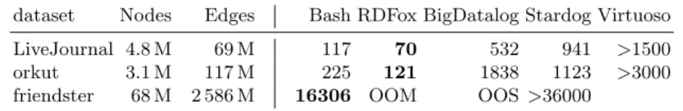
Setting. Our next datasets are the social networks LiveJournal [21], com-orkut [21], and friendster [19]. Table 3 shows the sizes of these datasets. We used a single query, which asks for all nodes that are reachable from a given node. As competitors, we chose again RDFox, Stardog, and Virtuoso. We could not use MonetDB or RDFSlice, because the reachability query is recursive. As an additional competitor, we chose BigDatalog [31]. This system was already run on the same LiveJournal and com-orkut graphs in the original paper [31]. We chose 3 random nodes (and thus generated 3 queries) for LiveJournal and com-orkut. We chose one random node for Friendster.
Results. Table 3 shows the average runtime for each system. Virtuoso was the slowest system, and we aborted it after 25min and 50min, respectively. We did not run it on the Friendster dataset, because Friendster is 20 times larger than the other two datasets. Stardog perfoms better. Still, we had to abort it after 10 hours on the Friendster dataset. BigDatalog performs well, but fails with an out of space error on the Friendster dataset. The fastest system is RDFox. This is because it can load the entire data into memory. This approach, however, fails with the Friendster dataset. It does not fit into memory, and RDFox is unable to run. Bash Datalog runs 50% slower than RDFox. In return, it is the only system that can finish in reasonable time on the Friendster dataset (4:32h).
dataset Nodes Edges Bash RDFox BigDatalog Stardog Virtuoso LiveJournal 4.8 M 69 M 117 70 532 941 >1500 orkut 3.1 M 117 M 225 121 1838 1123 >3000 friendster 68 M 2 586 M 16306 OOM OOS >36000
Table 3. Runtime for the reachability query, in seconds (OOM=Out of memory; OOS=Out of space).
5.3 YAGO and Wikidata
Setting. Our final experiments concern the knowledge bases YAGO [32] and Wikidata [35]. The YAGO data comes in 3 different files, one with the 12 M facts (814 MB), one with the taxonomy with 1.8 M facts (154 MB), and one with the 24 M type relations (1.6 GB in size). Wikidata is a single file of 267 GB with
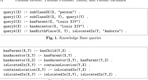
query1(X) :- subClassOf(X, "person") . query1(X) :- subClassOf(X, Y), query1(Y) . query2(X) :- hasParent(X, "Louis XIV") . query3(X) :- hasAncestor(X, "Louis XIV") .
query4(X) :- hasBirthPlace(X, Y), isLocatedIn(Y, "Andorra") . Fig. 1. Knowledge Base queries
hasParent(X,Y) :- hasChild(Y,X) . hasAncestor(X,Y) :- hasParent(X,Y) .
hasAncestor(X,Z) :- hasAncestor(X,Y), hasParent(Y,Z) . isLocatedIn(X,Y) :- containsLocation(Y,X) .
containsLocation(X,Y) :- isLocatedIn(Y,X) .
isLocatedIn(X,Y) :- isLocatedIn(X,Y), isLocatedIn(Y,Z) . Fig. 2. Knowledge Base rules
2.1 B triples. We designed 4 queries that are typical for such datasets (Table 1), together with a T-Box (Table 2).
Results. Table 4 shows the results of RDFox and our system on both datasets. On YAGO, RDFox is much slower than our system, because it needs to instan-tiate all rules in order to answer queries. On Wikidata, the data does not fit into main memory, and hence RDFox cannot run at all. Our system, in contrast, scales to the larger sizes of the data. One may think that a database system such as Postgres may be better adapted for such large datasets. This is, however, not the case. Postgres took 104 seconds to load the YAGO dataset, and 190 seconds to build the indexes. In this time, our system has already answered nearly all the queries.
YAGO Wikidata query Bash RDFox Bash RDFox
1 8 483 2259 OOM 2 5 483 2254 OOM 3 293 483 10171 OOM 4 5 481 2270 OOM
Table 4. Runtime for the Wikidata/YAGO benchmark in seconds. (OOM = out of memory error)
Discussion. All of our experiments evaluate only the setting that we consider in this paper, namely the setting where the user wants to execute a single query in order to preprocess the data. These are the cases that our system is designed for. We also want to emphasize again that our goal is not to be faster than all existing systems. This is not our point. Our point is that Bash Datalog can preprocess tabular data without the need to install any particular software. In addition, our approach is competitive in both speed and scalability to the state of the art.
6
Conclusion
In this paper, we have presented a method to compile Datalog programs into Unix Bash programs. This allows executing Datalog queries on tabular datasets without installing any software. We show that our method is competitive in terms of speed with state-of-the-art systems. Our system can be used online at https://www.thomasrebele.org/projects/bashlog, and the source code is available at URL. For future work, we aim to explore extensions of this work such as adding support of numerical comparisons to the Datalog language.
References
1. S. Abiteboul and R. Hull. Data functions, datalog and negation (extended ab-stract). In SIGMOD, 1988.
2. S. Abiteboul, R. Hull, and V. Vianu. Foundations of Databases. Addison-Wesley, 1995.
3. A. V. Aho and J. D. Ullman. The universality of data retrieval languages. In ACM Symposium on Principles of Programming Languages, 1979.
4. I. Alagiannis, R. Borovica, M. Branco, S. Idreos, and A. Ailamaki. Nodb: efficient query execution on raw data files. In SIGMOD, 2012.
5. P. A. Boncz, M. L. Kersten, and S. Manegold. Breaking the memory wall in monetdb. Communications of the ACM, 51(12), 2008.
6. Y. Bu, V. R. Borkar, M. J. Carey, J. Rosen, N. Polyzotis, T. Condie, M. Weimer, and R. Ramakrishnan. Scaling datalog for machine learning on big data. CoRR, abs/1203.0160, 2012.
7. P. Carbone, A. Katsifodimos, S. Ewen, V. Markl, S. Haridi, and K. Tzoumas. Apache flink. IEEE Data Eng. Bull., 38(4), 2015.
8. J. J. Carroll, I. Dickinson, C. Dollin, D. Reynolds, A. Seaborne, and K. Wilkinson. Jena: implementing the semantic web recommendations. In WWW, 2004. 9. F. Chang, J. Dean, S. Ghemawat, W. C. Hsieh, D. A. Wallach, M. Burrows,
T. Chandra, A. Fikes, and R. E. Gruber. Bigtable: A distributed storage sys-tem for structured data. ACM Transactions on Computer Syssys-tems, 26(2), 2008. 10. E. F. Codd. A relational model of data for large shared data banks.
Communica-tions of the ACM, 13(6), 1970.
11. O. Erling and I. Mikhailov. RDF support in the virtuoso DBMS. In Networked Knowledge, 2009.
12. M. K. et al. Impala: A modern, open-source SQL engine for hadoop. In CIDR, 2015.
13. J. D. Fern´andez, M. A. Mart´ınez-Prieto, C. Guti´errez, A. Polleres, and M. Arias. Binary rdf representation for publication and exchange (hdt). Web Semantics: Science, Services and Agents on the World Wide Web, 19, 2013.
14. Y. Guo, Z. Pan, and J. Heflin. LUBM: A benchmark for OWL knowledge base systems. J. of Web Semantics, 3(2-3), 2005.
15. V. Haarslev and R. M¨oller. RACER system description. In IJCAR, 2001. 16. S. Harris, A. Seaborne, and E. Prudhommeaux. SPARQL 1.1 query language.
W3C recommendation, 3 2013.
17. M. Isard, M. Budiu, Y. Yu, A. Birrell, and D. Fetterly. Dryad: distributed data-parallel programs from sequential building blocks. In EuroSys, 2007.
18. P. Katsogridakis, S. Papagiannaki, and P. Pratikakis. Execution of recursive queries in apache spark. In Euro-Par, 2017.
19. J. Kunegis. Konect: the koblenz network collection. In WWW, 2013.
20. N. Leone, G. Pfeifer, W. Faber, T. Eiter, G. Gottlob, S. Perri, and F. Scarcello. The DLV system for knowledge representation and reasoning. ACM Transactions on Computational Logic, 7(3), 2006.
21. J. Leskovec and A. Krevl. SNAP Datasets: Stanford large network dataset collec-tion. http://snap.stanford.edu/data, June 2014.
22. E. Marx, S. Shekarpour, T. Soru, A. M. P. Brasoveanu, M. Saleem, C. Baron, A. Weichselbraun, J. Lehmann, A. N. Ngomo, and S. Auer. Torpedo: Improving the state-of-the-art RDF dataset slicing. In ICSC, 2017.
23. B. Motik, B. C. Grau, I. Horrocks, Z. Wu, A. Fokoue, C. Lutz, et al. OWL 2 web ontology language profiles. W3C recommendation, 12 2012.
24. B. Motik, Y. Nenov, R. Piro, I. Horrocks, and D. Olteanu. Parallel materialisation of datalog programs in centralised, main-memory RDF systems. In AAAI, 2014. 25. B. Parsia and E. Sirin. Pellet: An owl dl reasoner. In ISWC, 2004.
26. T. Rebele, T. P. Tanon, and F. Suchanek. Technical report: Answering datalog queries with unix shell commands. Technical report, Telecom ParisTech, 2018. https://thomasrebele.org/.
27. M. Rogala, J. Hidders, and J. Sroka. Datalogra: datalog with recursive aggre-gation in the spark RDD model. In Int. Workshop on Graph Data Management Experiences and Systems, 2016.
28. B. Saha, H. Shah, S. Seth, G. Vijayaraghavan, A. C. Murthy, and C. Curino. Apache tez: A unifying framework for modeling and building data processing ap-plications. In SIGMOD, 2015.
29. M. Shaw, P. Koutris, B. Howe, and D. Suciu. Optimizing large-scale semi-na¨ıve datalog evaluation in hadoop. In Int. Workshop on Datalog in Academia and Industry, 2012.
30. R. Shearer, B. Motik, and I. Horrocks. Hermit: A highly-efficient owl reasoner. In OWLED, volume 432, 2008.
31. A. Shkapsky, M. Yang, M. Interlandi, H. Chiu, T. Condie, and C. Zaniolo. Big data analytics with datalog queries on spark. In SIGMOD, 2016.
32. F. M. Suchanek, G. Kasneci, and G. Weikum. Yago: a core of semantic knowledge. In WWW, 2007.
33. D. Tsarkov and I. Horrocks. Fact++ description logic reasoner: System description. Automated reasoning, 2006.
34. R. Verborgh, M. Vander Sande, O. Hartig, J. Van Herwegen, L. De Vocht, B. De Meester, G. Haesendonck, and P. Colpaert. Triple Pattern Fragments: a low-cost knowledge graph interface for the Web. J. of Web Semantics, 37–38, Mar. 2016.
35. D. Vrandecic and M. Kr¨otzsch. Wikidata: a free collaborative knowledgebase. Communications of the ACM, 57(10), 2014.
36. J. Wang, M. Balazinska, and D. Halperin. Asynchronous and fault-tolerant recur-sive datalog evaluation in shared-nothing engines. PVLDB, 8(12), 2015.
37. H. Wu, J. Liu, T. Wang, D. Ye, J. Wei, and H. Zhong. Parallel materialization of datalog programs with spark for scalable reasoning. In WISE, 2016.
38. M. Zaharia, M. Chowdhury, M. J. Franklin, S. Shenker, and I. Stoica. Spark: Cluster computing with working sets. In USENIX Workshop on Hot Topics in Cloud Computing, 2010.
39. J. Zhou, P. Larson, and R. Chaiken. Incorporating partitioning and parallel plans into the SCOPE optimizer. In ICDE, 2010.