Comparison and validation of risk assessment tools (FRAC-WECO Deliverable D4.1)

(1)

CONTRACT NB SD/TE/02A FRAC-WECO

Flux-based Risk Assessment of the impact of Contaminants on Water resources and ECOsystems

Programme: La Science pour un Développement Durable Programma: Wetenschap voor een Duurzame Ontwikkeling

Deliverable D4.1

Comparison and validation of risk assessment tools

Responsible D.Caterina, J. Batlle-Aguilar, S.Brouyère (ULg HG)

Contributors A.Dassargues

Corresponding authors: David.Caterina@ulg.ac.be, Tel: +32 4 366 92 62 Serge.Brouyere@ulg.ac.be, Tel: +32 4 366 23 77 Alain.Dassargues@ulg.ac.be, Tel: +32 4 366 23 76

(2)

i

List of tables

Table 1 : Parameters used for simulations on the Sclaigneaux case study ... 28

Table 2 : Evolution of mercury concentrations at the receptor with the loam layer ... 30

Table 3 : Evolution of mercury concentrations at the receptor with the loam layer ... 31

Table 4 : Parameters used for simulations on the Flémalle case study ... 34

List of figures

Figure 1 : Schema showing the conceptual model implemented in MISP ... 3

Figure 2 : Conceptual model of tools (such as RBCA Toolkit) using a mixing layer (Guyonnet, 2008) ... 4

Figure 3 : Conceptual model implemented in RBCA Toolkit ... 11

Figure 4 : Schematic view of vertical transport through the vadose zone and associated parameters in RBCA Toolkit (Connor & al., 2007) ... 13

Figure 5 : Schematic view of transport in the aquifer and associated parameters (Connor & al., 2007) ... 14

Figure 6 : Tiered approach implemented in RTWS (Carey & al., 2006) ... 21

Figure 7 : The Sclaigneaux site ... 24

Figure 8 : Conceptual model of the Sclaigneaux site with loam layer ... 26

Figure 9 : Conceptual model of the Sclaigneaux site without the loam layer... 26

Figure 10 : The Flémalle site ... 32

Figure 11 : Conceptual model of the Flémalle site ... 33

Figure 12 : Benzene concentration evolution at a “control plane” located 20 m downstream from one of the main sources of benzene ... 35

(4)

iii

List of acronyms

ANZECC Australia and New Zealand Environment and Conservation Council ASTM American Society for Testing and Materials

BP British Petroleum

BRGM Bureau de Recherches Géologiques et Minières FIELDS Field Environmental Decision Support

GIS Geographic Information System

GMS Groundwater Modelling System

MISP Model for estimating the Impact of Sources of Pollutants NOAA _{National Oceanic and Atmospheric Administration}

RA Risk Assessment

RAGS Risk Assess Guidance for Superfund RBCA Risk-Based Corrective Action

RISC Risk-Integrated Software for Clean-ups

RT3D Three-dimensional, multi-species, reactive transport model

RTWS Remedial Targets Worksheet

SADA Spatial Analysis and Decision Assistance

(5)

1

1. Introduction

The objective of this document is to review a series of risk assessment tools that were selected in Deliverable 2.5: Decision grid for best approach in terms of modelling concepts/ contaminants. As a reminder, the selection was carried out as follows:

First, most cited risk assessment tools (RA tools) in the literature were selected. In a second step, about thirty softwares were chosen according to their characteristics and their potential usefulness in the scope of the project. The criteria that were taken into account in the selection process are the:

• type of risk concerned (risk on water resources and ecosystems);

• type of contaminants managed by the software (at least the most common ones: hydrocarbons, heavy metals, chlorinated solvents and semi-organic volatile compounds...);

• type of media managed by the software (soil, groundwater and surface water);

• possibility to take into account in a certain way the contaminant fluxes data (hydraulic conductivity, hydraulic gradient, ...);

• possibility to take into account attenuation factors (partitioning between the liquid-, solid- and gaseous phases; re-distribution in the soil profile by sorption; dilution in groundwater; biodegradation);

• complexity of the models (analytical or numerical); • possibility to use GIS data;

• type of inputs and outputs;

• possibility to calculate uncertainty on the results;

• possibility to calculate cost-benefit from remedial action. Based on these criteria, several tools have been selected:

• RISC Workbench (http://www.bpRISC.com/index.htm);

(6)

2 In the scope of this document, additional tools have also been included in the selection in order to be tested further. :

• MISP (http://www2.brgm.fr/MISP/);

• Remedial Targets Worksheet (

http://www.environment-agency.gov.uk/subjects/landquality/113813/887579/887905/?lang=_e).

Note that SADA (http://www.tiem.utk.edu/~sada/index.shtml) and FIELDS

(http://epa.instepsoftware.com/fields/), initially selected in deliverable 2.5, will not be described in this document because it turned out that they do not have the necessary characteristics to study the transport of dissolved contaminants.

This document is organized as follows. First, a description of selected softwares via their ability to model the transport of dissolved contaminants. Second, a presentation of the two case studies on which each tool will be tested and compared to others. Third, the comparison of results in itself and finally, conclusions and perspectives of the study will be drawn.

(7)

3

2. Description of softwares

2.1. MISP

MISP software developed by BRGM is an analytical model, in free-access, which calculates the impact on groundwater of a pollutant source located above the water table. It combines, through convolution, a solution for vertical migration through a layer overlying the aquifer, with the solution of Galya (1987) for 3-dimensional transport from a patch source at the water table surface (Guyonnet, 2008). MISP does not contain chemical/toxicological and hydrogeological databases, so that all parameters needed for simulations have to be entered manually in the input file. MISP does not also calculate any ‘risk’ factor.

2.1.1 Conceptual model

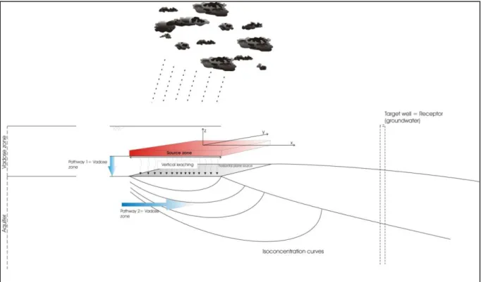
MISP is designed to model the transport of contaminant in both the unsaturated (vadose) and saturated (aquifer) layers as shown in Figure 1. However, it also allows considering the transport of contaminant only in the saturated layer by choosing the appropriate option in the input file.

(8)

4 Evolution of concentration is calculated in a well (named ‘target well’ in Figure 1) located downstream of the source of contaminant.

The axis system is defined in Figure 1.

Unlike other analytical models, MISP does not assume the existence of a mixing layer below the source zone. The assumption of a mixing layer implies that the contaminant flux emanating from the source zone is mixed homogeneously and instantaneously over this mixing layer. This idealised mixing provides a groundwater concentration beneath the source area, which becomes a boundary condition for transport in the groundwater (Guyonnet, 2008).

Figure 2 : Conceptual model of tools (such as RBCA Toolkit) using a mixing layer (Guyonnet, 2008)

The problem with that approach is that such a mixing does not represent the reality. Indeed, the real mixing is something more gradual that involves several complex processes.

This is why developers of MISP have chosen to adopt another concept proposed by Galya (1987). This author used Green’s functions to derive a solution for the 3-dimensional advective-dispersive transport of dissolved contaminants in an aquifer with a uniform velocity field, resulting from a uniform flux input at the surface of the water table (Guyonnet, 2008).

(9)

5

2.1.2 Theory

2.1.2.1 Theory of convolution

As mentioned in the introduction, MISP combines through convolution a solution for vertical transport from a source located at the top of a layer overlying the aquifer with the solution of Galya for three-dimensional transport from a plane source at the water table.

The evolution of contaminant concentration in the aquifer in function of time t can be expressed by the following equation considering a constant source concentration .

(2.1.1)

Where,

• is a function of spatial coordinates and of time,

• constant source concentration [-].

If the source concentration is variable over time, concentration in the aquifer over time will depend of the concentration values taken by the source.

(2.1.2)

Where,

• is the number of levels by which the source concentration varies,

• are mass fluxes of pollutant at the interface between the unsaturated and the saturated zones below the source of contaminant.

In MISP, the function F can be seen as the solution of Galya for the 3D transport in the aquifer.

2.1.2.2 Solution for the vertical transport in the unsaturated zone

The vertical migration through the unsaturated layer is governed by the following processes: • advection in one dimension;

• dispersion-diffusion;

(10)

6 • degradation (first order decay).

(2.1.3)

With,

• i the net recharge (=infiltration rate) [L/T], • the volumetric water content [-],

• D the diffusion-dispersion coefficient [L²/T],

• the retardation factor [-], with

o the soil bulk density [M/L³],

o the partition coefficient of pollutant between the solid phase and the liquid phase [L³/M],

• the first order decay rate of the contaminant [T-1].

The diffusion-dispersion factor is expressed by the following equation:

(2.1.4)

Where,

• is the longitudinal dispersivity [L],

• is the free-solution diffusion coefficient [L²/T], • is the tortuosity [-].

To resolve equation (2.1.3), definition of top and bottom boundary conditions in the unsaturated layer is required. An initial condition is also required and assumes a zero concentration in the entire layer.

MISP proposes five options for the top boundary conditions (Guyonnet, 2008):

• the first option does not consider any unsaturated layer. A constant mass flux over a specified area enters the aquifer at the water table. With this option, MISP is reduced to the solution of Galya (1987);

(11)

7 • the second option considers that a constant source concentration with a specified

duration is applied at the top of the layer;

• the third option considers a source concentration at the top of the layer that decreases exponentially;

• the fourth option considers that the concentration at the source located at the top of the layer is defined by diffusive release from a solidified slab of waste;

• the fifth option considers that the source concentration is given in a separate file provided by the user.

For the boundary conditions at the bottom of the unsaturated layer, a mass balance is performed over a thin portion of aquifer below the source area. The mass balance is written as:

(2.1.5)

Where,

• H is the thickness of the bottom boundary layer [L],

• L is the length of source in the direction of groundwater flow [L], • is the aquifer porosity [-],

• c* (t) is the concentration in the aquifer beneath the source zone in a boundary layer [M/L³],

• e is the thickness of the unsaturated layer [L],

• qu is the Darcy flow in the aquifer just beneath the source zone [L/T],

• is the first-order decay rate of contaminant in the aquifer [T-1].

The mass flux of contaminant between the unsaturated layer and the water table is then fed into Galya’s solution for estimating the aquifer concentration downstream.

Guyonnet & al. (1998) proposed a solution for the equation (2.1.5) expressed in the Laplace space:

(12)

8 With,

• Where,

• is the concentration in the boundary layer expressed in the Laplace space [M/L³];

• is the Laplace variable;

• is the first-order decay rate for the source concentration [T-1].

With the equations (2.1.5) and (2.1.6), the mass flux between the unsaturated layer and the aquifer can be expressed as:

(2.1.6)

2.1.2.3 Solution for transport in the aquifer

As already stated, the solution of Galya is used to model the transport in the saturated zone. The equation resolved by Galya is the following:

(2.1.7)

Where,

• is the concentration in the aquifer in function of space and time [M/L³], • is the retardation factor in the aquifer [-],

• , and are respectively longitudinal, horizontal-transverse and vertical-transverse diffusion-dispersion coefficients [L²/T],

• is the mass flux at the water table (equivalent to ) [M/T].

To resolve this equation, initial and boundary conditions are needed. The initial condition just consists in considering a zero concentration in the aquifer at t = 0.

(13)

9 The boundary conditions are:

• C(x, y, z, t) = 0 for x = or y =

• for z = 0 (at the water table)

• for z = HT (where HT is the total thickness of the aquifer in meters)

The Galya’s solution is expressed with the functions of Green:

(2.1.8)

With,

• T a degradation function • an integration variable

• are functions of Green

(2.1.9) (2.1.10) (2.1.11) (2.1.12) Where,

• B is the width of the contaminant source [L], • v is the groundwater velocity [L/T],

(14)

10

2.2. RBCA Toolkit v2.0

The RBCA Toolkit software developed by GSI Environmental is a modelling and risk characterization software package designed to support Risk-Based Corrective Action at contaminated sites. The Risk-Based Corrective Action is a decision making process for the assessment and response to chemical releases. The RBCA Toolkit software is specially designed to complete all calculations required for Tiers 1 and 2 of the ASTM-RBCA planning process, as defined in ASTM E-2081-00 Standard Guide for Risk-Based Corrective Action (ASTM, 2004) and ASTM E-1739-95 Standard Guide for Risk-Based Corrective Action Applied at Petroleum Release Sites (ASTM, 2002). (Connor & al., 2007)

RBCA Toolkit is designed to work under Microsoft® Excel (versions 2000 through 2003) environment.

The RBCA Toolkit software contains (customisable) chemical/toxicological database for over 600 compounds, including default toxicity dose-response parameters coming from official sources in the United States, Netherlands and United Kingdom. The database is customizable by the users. The package also includes analytical models for air, groundwater, and soil exposure pathways, including all models used in ASTM RBCA standards. In the following sections, the analytical model for groundwater exposure pathway will be described more in details.

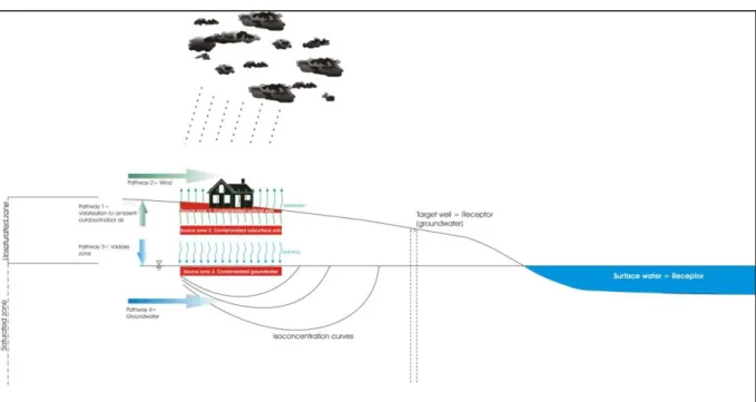
The conceptual model implemented in the RBCA Toolkit software is built on the Source-Pathway-Receptor (SPR) approach. As shown in Figure 3, RBCA allows considering multiple pathways for the transport of contaminants from a specified source. A summary of main elements of the SPR considered in RBCA is presented below.

Sources

• Affected surface soils (source 1) • Contaminated soils (source 2)

• Contaminated groundwater (source 3)

Pathways

(15)

11 • Air: transport of contaminated air/particles by wind (pathway 2)

• Vadose zone: transport of contaminants to the water table zone through the unsaturated zone by leaching (pathway 3)

• Groundwater: transport of dissolved contaminants through groundwater (pathway 4)

Receptors

• Groundwater

• Humans: via dermal contact, incidental ingestion, inhalation of vapours and dust, and vegetable ingestion

• Surface water: as impacted by the discharge of groundwater (human exposure via swimming or fish consumption, and direct exposure of humans or aquatic species)

Figure 3 : Conceptual model implemented in RBCA Toolkit

For this document, it is foreseen to focus only on the sources 2 and 3, on the pathways 3 and 4, and on groundwater as a receptor.

2.2.2 Theory

In RBCA Toolkit, a soil to groundwater Leaching Factor (LF) is used. LF represents the steady state ratio of the predicted concentration of a chemical constituent in groundwater to the source concentration in overlying affected soil (Connor & al., 2007). LF can be introduced manually by the user or calculated with the following equation:

(16)

12

(2.2.1)

Where,

• is the soil-water partition factor [M/L³], with

o the volumetric water content in vadose zone soils [-], o the soil-water sorption coefficient= foc.koc [-],

o the Henry’s law constant [-].

is used to represent the release of soil constituents to leachate percolating through the affected soil zone (Connor & al., 2007).

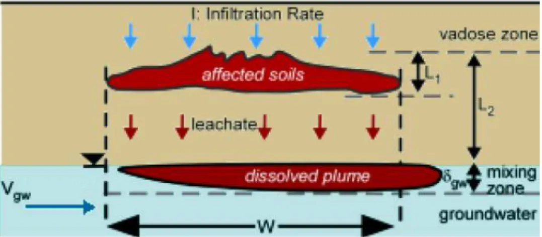
• is the (optional) Soil Attenuation Model factor [-], see Figure 4.

is used to take into account the possibility of adsorption of leachate by clean soils underlying the source zone.

• is the Leachate Diluton Factor [-], with

o the groundwater Darcy velocity [L/T],

o the net recharge (=infiltration rate) [L/T],

o the width of the source area parallel to groundwater flow [L],

o the groundwater mixing

zone thickness [L], where b is the aquifer saturated thickness [L].

LDF accounts for the dilution occurring when the leachate reaches the water table and mixes with groundwater.

It is important to notice that LDF can be linked with equation (2.1.7). Indeed, as explained in Guyonnet (2008), the final value theorem (Churchill, 1958),

(17)

13 (2.2.2)

If the exponential term (which represents the diffusive-dispersive component) is not taken into account in the previous equation, it becomes:

(2.2.3)

This gives,

(2.2.4)

With the suitable adaptation in used symbols.

Figure 4 : Schematic view of vertical transport through the vadose zone and associated parameters in RBCA Toolkit (Connor & al., 2007)

RBCA Toolkit software uses the Domenico (1987) analytical solution to model the transport of contaminant in the aquifer. The Domenico’s model uses a vertical plane source (= Groundwater Source Term Location in Figure 5), perpendicular to groundwater flow, to simulate the release of contaminants (assumed to be constant in RBCA) from the mixing zone to the aquifer. Though the Domenico model can predict steady-state plume concentrations at any point (x, y, z) in the downgradient flow system, RBCA Toolkit is only set to predict

(18)

14 centreline plume concentrations at any downgradient distance x. The receptor well is thus supposed to be located on the plume centreline.

The model takes into account the advection, dispersion, sorption, and biodegradation processes.

Hydrogeologic parameters such as: hydraulic conductivity, hydraulic gradient and effective porosity have to be entered manually by the user in the interface. Dispersion coefficients can be entered either manually or calculated following two different relationships: ASTM E-1739 (1995) or Xu and Eckstein (1995).

Figure 5 : Schematic view of transport in the aquifer and associated parameters (Connor & al., 2007)

The Domenico’s solution with first-order decay is presented in the next equation:

(2.2.5) Where:

(19)

15 o the hydraulic conductivity of the aquifer [L/T],

o _{the hydraulic gradient in the aquifer [-],} o the effective porosity of the aquifer [-],

• is first-order decay rate for the specified contaminant [T-1] and can be entered manually by the user or provided by the chemical database included in the software,

• is the retardation factor in the aquifer [-],

• and are respectively the groundwater source term width and thickness [L], see Figure 5.

A solution accounting for the biodegradation by electron-acceptor superposition method is also available in the software (see Connor & al. (2007) for more information).

2.3. RISC Workbench

Risk-Integrated Software for Cleanups (RISC) was developed by BP Oil to assess potential risk on human health due to contaminated sites. However, it can be used for three others main applications: estimate risk-based cleanup levels in various media, perform simple fate and transport modelling and evaluate potential impacts to surface water and sediments of a chemical release (Spence & al., 2001).

The assessment of risk on human health in RISC Workbench is based on US EPA’s Risk Assessment Guidance for Superfund, RAGS (US EPA, 1989). RAGS divides the risk assessment process into four main steps: 1) data collection an evaluation, 2) exposure assessment, 3) toxicity assessment and 4) risk characterization. RISC Workbench is designed to account for the processes 2) to 4), assuming that the data collection and evaluation process has already been performed.

To estimate risk-based cleanup levels (= concentrations of contaminants that pose an acceptable risk if they are left in place), RISC uses the guidelines published in ASTM E1739-95, Standard Guide for Risk-based Corrective Action Applied at Petroleum Release Sites. The fate and transport model incorporated in RISC Workbench will be described in the next sections.

RISC Workbench contains a database for surface water quality criteria coming from different countries: United States Environment Protection Agency Ambient Water Quality Criteria, United Kingdom Environmental Quality Standards, Australia and New Zealand Environment

(20)

16 and Conservation Council (ANZECC) Guidelines for the Protection of Aquatic Ecosystems, European Commission Water Quality Objective, and Canadian Council of Ministers for the Environment Freshwater Aquatic Life Guideline (Spence & al., 2001). The sediment criteria database is from the United States National Oceanographic and Atmospheric Administration (NOAA).

RISC Workbench also contains a (customisable) chemical/toxicological database for 87 components.

The conceptual model implemented in RISC Workbench is similar to the one implemented in RBCA Toolkit (see section 2.2.1). Differences arise concerning the equations and processes used to model the transport of contaminant both in the unsaturated and saturated zones.

2.3.2 Theory

The solution implemented in RISC Workbench to account for the vertical transport of contaminants in the unsaturated zone is the analytical solution of the one-dimensional advective-dispersive solute transport equation proposed by Van Genuchten & Alves (1982). The equation resolved is:

(2.3.1)

Where,

• is the retardation factor in the unsaturated zone[-], with

o the fraction of organic carbon in soil [-],

o the organic carbon normalized partition coefficient [M/L³], o the volumetric water content [-],

• is the concentration of dissolved contaminant at the distance x (expressed in

meters) below the source zone [M/L³],

(21)

17 o longitudinal dispersivity [L],

• is the seepage velocity [L/T],

• is the first-order decay coefficient [T-1].

To resolve the equation (2.3.1), initial and boundary conditions are needed. At time t=0, concentrations are set to zero below the source:

(2.3.2)

The source concentration is supposed to decrease exponentially to account for the mass loss of contaminants with time.

(2.3.3)

• is the concentration of dissolved contaminant in the source at t=0

[M/L³], with:

o the concentration of contaminant in the soil [M/M],

o the partition coefficient of pollutant between the solid and liquid phases [L³/M],

o the air filled porosity in the vadose zone [-], o the Henry’s constant [-],

• is the source zone depletion coefficient [-],

where:

o is the net recharge (= infiltration rate) [L/T],

o is the effective diffusion coefficient in the unsaturated zone [L²/T], o is the thickness of the source area [L],

o is the diffusion path length [L].

(22)

18 With the defined conditions, the solution of equation (2.3.1) proposed Van Genuchten and Alvès (1982) is:

(2.3.4) Where,

• , with:

o

The concentrations calculated at the water table are combined with the net recharge to estimate the mass flux of contaminant loading to groundwater.

The equation solved for the transport in the aquifer accounts for the processes of advection, dispersion-diffusion, adsorption and degradation as shown in equation (2.3.5).

(2.3.5) Where,

• is the mass loading rate in the aquifer [M/T],

• , , are respectively longitudinal, transverse and vertical

dispersion coefficients [L²/T], with

o and dispersivity in x, y and z directions [L], o the Darcy velocity in the aquifer [L/T].

The other terms are similar to those described in the previous section unless they are related to the properties of the aquifer, rather than the unsaturated zone.

Dispersivities can be entered by the user or calculated in the program with the following equation:

(23)

19 (2.3.6) Where x is the distance from the source to the receptor (Gelhar & al., 1985).

,

and are respectively equal to 3 and 87 (American Petroleum Institute, 1987).

The solution used to resolve the equation (2.3.5) is the Galya’s solution (1987) already described in section 2.1.2.3.

2.4. Remedial Targets Worksheet

The Remedial Targets Worksheet v3.0 (RTWS) developed by the Environment Agency (United Kingdom) is a Microsoft® Excel based tool which is designed to help assessors to derive site-specific remedial targets for contaminated soils and groundwater that are protective of the wider environment (Smith & al., 2006). In other words, the user has to define a “target concentration CT” at a defined receptor (= a well) that should not be exceeded and the software computes a “remedial target RT” that represents the concentration of the source that produces CT at the receptor. However, RTWS also allows calculating profile of concentrations at a given time for a specified source concentration.

RTWS does not contain any chemical/toxicological and hydrogeological databases. The user has thus to enter manually the chemical properties of the contaminants. In addition, RTWS does not calculate any “risk factor”. In this way, results that it provides are similar to those of the MISP software.

RTWS works on the basis of a tiered approach. At each further level, the need of data coming from the site grows. The idea is to use the software throughout the study to refine the calculation of RT and so define more precisely the proportion of the site to clean up based on additional information acquired.

Three levels are implemented in the software: • Level 1

No attenuation factor and no dilution are taken into account. The source concentration will not be diminished at the receptor point.

(24)

20 (2.4.1) • Level 2

A dilution factor (DF) is taken into account at the interface between the unsaturated zone and the groundwater table. This means that, at the receptor point located beyond this interface, the concentration of contaminant will be lower than at the source.

(2.4.2) • Level 3

A dilution and an attenuation factor (AF) are taken into account. AF occurs during the transport of contaminant in the saturated zone.

(2.4.3) Figure 6 summarizes these different concepts.

(25)

21

Figure 6 : Tiered approach implemented in RTWS (Carey & al., 2006)

2.4.2 Theory

The source concentration is constant throughout the simulation. No notion of travel time is taken into account in the levels 1 and 2.

As already explained, only a dilution factor DF is considered to model the vertical transport of contaminant in the unsaturated zone in levels 2 and 3. The expression of DF is the following:

(26)

22 (2.4.4)

Where,

• K is the hydraulic conductivity of the aquifer [L/T], • is the hydraulic gradient in the aquifer [-],

• is the thickness of the mixing layer (US

EPA, 1996) [L], with

o the length of the source in the direction of the groundwater flow [L], o the thickness of the aquifer [L],

o the net recharge (= infiltration rate) [L/T],

o the natural background concentration of contaminant [M/L³].

The attenuation factor AF introduced for the transport in the aquifer (see equation 2.4.5) includes the following processes: dispersion, adsorption, degradation, ion exchange, precipitation of inorganic compounds and volatilization.

(2.4.5)

Where,

• is the dissolved contaminant concentration in the aquifer just below the source [M/L³],

• is the computed dissolved contaminant concentration at the receptor [M/L³]. To calculate , RTWS proposes different solutions for the transport in the saturated zone: the Ogata Banks solution (1961) and the Domenico’s solution (1987).

(27)

23 Ogata Banks solution

(2.4.6)

Where,

• ax , ay, az are respectively longitudinal, vertical and lateral dispersivities [L],

• is the first-order decay rate of the contaminant [T-1],

• u is the rate of contaminant movement due to retardation (adsorption) [L/T], with

o the effective porosity of the aquifer [-],

o the retardation factor already defined in the previous sections [-], • x,y,z are distances from the source zone to the receptor [L],

• Sz , Sy are width and thickness of plume at source in the saturated zone [L],

• is an error function,

• is a complementary error function,

• is the time since contaminant entered groundwater [T]. Domenico’s solution

The Domenico’s solution is a simplification of the Ogata Banks solution.

(28)

24

3. Case Studies

It has been decided to test the previously described tools on two case studies: the “Carrières et Fours de Sclaigneaux” and the “Cokerie Flémalle” sites1.

3.1. Sclaigneaux site

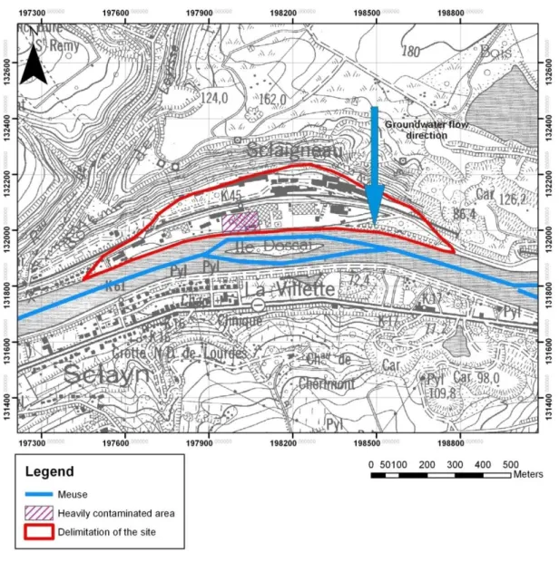
3.1.1 Introduction

The Sclaigneaux site lies in the alluvial plain of the Meuse River (left bank) near the city of Andenne. Figure 7 shows the delimitation of the site.

Figure 7 : The Sclaigneaux site

(29)

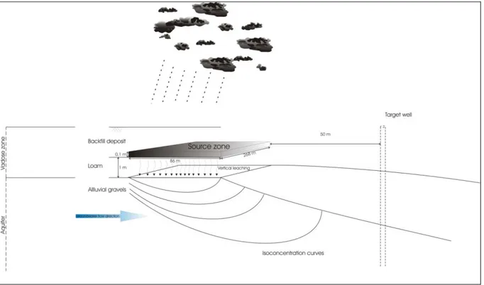
25 The geology of the site can be seen as follows:

• a top layer of backfill deposits whose thickness is between 1 and 7 meters;

• an intermediate layer of loam (Quaternary) with a thickness between 0 and 4 meters; • a bottom layer of alluvial gravels (Quaternary) with a thickness between 2 and 6

meters.

Below these layers, lie dolomites and limestones from the Primary (thickness between 3,5 and 12 meters).

The site is contaminated mainly with mercury whose origin seems to be linked to the nature of the backfill layer. Some areas of the site are more contaminated than others. For this report, it has been decided to focus the study on the main contaminant area (see hatched polygon in Figure 7).

In order to be able to compare results coming from all tested softwares, it is necessary for them to work on the same basis. It is thus important to define a conceptual model of the Sclaigneaux site that will be implemented in each tool.

As tested softwares do not allow to model complex situations, strong simplifications of the reality are needed. Among others, the source zone of contaminant will be considered as a parallelepiped rectangle with a length of 86 meters in the direction of groundwater flow, a width of 200 meters perpendicular to that direction and a thickness of 0,1 meter. This source zone will lie in the bottom of the backfill layer with the same hydrogeological properties as it. Below the backfill layer, a loam layer of 1 meter thick will be modelled. Due to the fact that in reality, this layer is not present everywhere on the site, it has been decided to also study the case where the loam layer does not exist.

The alluvial gravels of the Meuse River will be considered as the aquifer with a thickness of 5 meters.

The migration of the pollutant in the aquifer will be observed in a receptor well located 50 meters downstream from the source zone.

(30)

26 Figure 8 shows the conceptual model of the site with the loam layer while Figure 9 shows the conceptual model without that layer.

Figure 8 : Conceptual model of the Sclaigneaux site with loam layer

(31)

27

3.1.3 Choice of parameters

Parameters that will be used in the model come from several sources. Some are coming from the exploratory analysis (dimension of the source zone, concentration in mercury, hydraulic gradient…), some are coming from default values proposed by tested softwares and finally some are coming from literature.

Infiltration

Tested tools do not allow to model two different water tables. They just allow modelling one saturated zone below an unsaturated one. However, it appears that, on the Sclaigneaux site, there is a superficial water table located in the backfill deposits that is in charge compared to the water table located in the gravels. In order to take into account the difference of level between both, it was decided to put the source of contaminant in the unsaturated zone and to simulate the difference of level by an infiltration which not only takes into account the precipitations but also the water flow between the two layers due to that difference. The flux is calculated as follows:

(3.1.1)

Where:

• q is the Darcy flux through the intermediary layer [L/T],

• Kint. layer is the hydraulic conductivity of the intermediary layer [L/T],

• hint.layer and hgravels are the piezometric heads in the intermediary layer and in the gravels layer [L].

Retardation factor

The calculation of retardation factor for each layer is performed via the following equation:

(3.1.2)

Where:

(32)

28 • Kd is the partition coefficient of pollutant between the solid and liquid phases [L³/M], • is the bulk density of the layer [M/L³],

• is the effective porosity of the layer [-].

Table 1 summarizes all the parameters used in the simulations for Sclaigneaux site.

Description Value Units Origin

Source zone

Length 86 m Exploratory analysis1

Width 200 m Exploratory analysis1

Thickness 0,1 m Exploratory analysis1

Receptor

well Distance from the source zone 50 m User's choice

Backfill

Thickness 3 m Exploratory analysis1

Effective porosity (ne) 0,025 - Default value in RISC Workbench

Hydraulic conductivity (K) 10-4 m/s Literature2

Tortuosity coefficient - -

Degradation constant (λ) 0 s-1 User's choice3

Retardation factor (R) 10473 - Calculation4

Loam

Thickness 1 m Exploratory analysis1

Effective porosity (n_e) 0,015 - Default value in RISC Workbench

Hydraulic conductivity (K) 10-6 m/s Litterature2

Coefficient of tortuosity 0,15 - Default value in RISC Workbench

Gravels

Thickness 5 m User's choice

Effective porosity (ne) 0,02 - Literature

5

Hydraulic conductivity (K) 10-3 m/s Literature2

Coefficient of tortuosity 0,67 -

Hydraulic gradient (i) 10-3 Field data6

Longitudinal dispersivity (aL) 8,32 m Literature

5

Transversal dispersivity (aT) 0.832 m User’s choice

Mercury

Concentration in the source zone 10 mg/l Exploratory analysis

Distribution coefficient 154 l/kg Default value in RISC Workbench

Diffusion coefficient in water 6,3.10-6 m²/s Default value in RISC Workbench

Table 1 : Parameters used for simulations on the Sclaigneaux case study

1_{(SGS Belgium, 2003)}

2_{(Domenico P. & Schwartz f., 1998)}

3_{Value chosen to be on the safety side}

4_{See equation 2.2}

5_{(Aquaterra, 2006)}

(33)

29

3.1.4 Estimate of transport time

An estimate of the time taken by the mercury to cross the intermediary layer and then to reach the target well can be made taking into account the advection and the retardation processes. This estimate allows having an idea of the time scale that should cover simulations and the general aspect of expected results.

For example, if an intermediary layer of loam is considered, the time needed by the pollutant to cross it, is given by:

This corresponds to approximatively 11 years. The same approach can be used to calculate the travel time in the aquifer to the target well.

This corresponds to approximatively 415 years.

In the case where the loam layer is absent, the time for the pollutant to cross the intermediate layer (same properties as backfills) is reduced to 40 days. The travel time in the aquifer stays unchanged.

3.2. Comparison and validation of results for the Sclaigneaux

case study

3.2.1 Results

The main idea behind the choice of the Sclaigneaux site as a case study is to compare and explain results provided by the different tools following their capacity of modelling the transport of dissolved contaminants in the unsaturated zone and in the saturated zone. Unfortunately, no variably saturated and transport numerical model is available for this case study. The comparison will just be based on the results of analytical models. No validation is thus possible for the moment.

(34)

30

Results with the loam layer

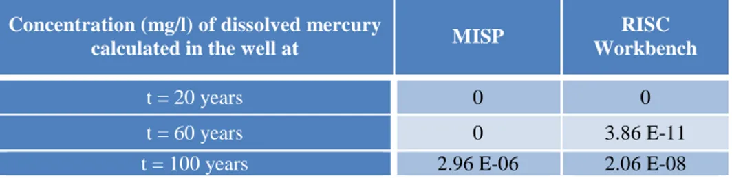
Only MISP and RISC Workbench softwares allow considering two layers with different properties in the unsaturated zone, as shown in Figure 8. Simulations with the loam layer below the backfill deposits were thus run only on these two tools. .

As RISC Workbench allows only simulations with a maximum duration of 100 years, comparison is limited to that period of time.

Concentration (mg/l) of dissolved mercury

calculated in the well at MISP

RISC Workbench

t = 20 years 0 0

t = 60 years 0 3.86 E-11

t = 100 years 2.96 E-06 2.06 E-08

Table 2 : Evolution of mercury concentrations at the receptor with the loam layer

As shown in Table 2, there are some differences between the results provided by the two softwares. The first one is that the concentration computed by MISP after 100 years is two order of magnitude higher than concentration computed by RISC Workbench. The second difference is that the first arrival of contaminant appears sooner with RISC Workbench than with MISP.

The equation used to model the vertical transport of contaminant is the same for both software (same processes taken into account) and the solution used to model the transport in the aquifer is also the same (Galya). Differences in results are thus probably not due to these equations. RISC Workbench accounts for the volatilization of a portion of the contaminant source while MISP does not. In all logic, it is therefore normal that concentration computed by RISC Workbench at the receptor point is lower than concentration computed by MISP. However, the cumulated volatilization losses during the 100 years of the simulation amount only to 0.00199 kg of mercury. This only represents a thousandth of the total mass of mercury available (4,7 kg). Volatilization losses can thus not explain alone such differences in the magnitude of results.

Another explanation of that behaviour is that RISC Workbench works with a finite mass of contaminant in the source that depletes with time. MISP considers a constant contaminant source concentration during the simulation. To compare the two softwares in a better way, another simulation was run in MISP with the activity of the source limited to one year. With

(35)

31 this new input, the concentration reached in the receptor well after 100 years amounts to 3,17E-7 mg/l, one order of magnitude higher than RISC Workbench.

These are the pieces of information that can be provided at this stage to explain the differences of results observed.

Results without the loam layer

The four tested tools are able to model the transport of contaminant without the intermediary loam layer. Results obtained by the different simulations are provided in Table 3 for a period of 200 years.

Concentration (mg/l) of dissolved mercury calculated in

the well at

MISP RBCA Toolkit RISC Workbench RTWS

t = 20 years 0 0 0 0

t = 60 years 7.7 E-6 0 0 0

t = 100 years 7.8 E-4 0 0 5.19 E-06

t = 150 years 0.016 3.4 E-14 - 1.57 E-5

t = 200 years 0.068 9.1 E-9 - 1.69 E-5

Table 3 : Evolution of mercury concentrations at the receptor with the loam layer

Once again, results appear to be quite different depending on the software used. MISP shows the first arrival and the higher concentration of contaminant. Other tools present concentrations much lower (several orders of magnitude) than MISP at the end of the simulation. Compared to the case where the loam layer is intercalated between the source and the aquifer, results provided by MISP indicate that the loam layer plays a protective role, retarding the migration of pollutant from the source to the aquifer. On the other hand, RISC Workbench shows no arrival of pollutant after 100 years while when the loam layer was present, it begins to show first arrival of contaminant after 33 years. This behaviour is the contrary of results provided by MISP and may seem illogic.

The main difficulty related to the interpretation of these simulations lies in the fact that there are no “validated results” (calibrated numerical model) from which a more detailed interpretation would be possible. Until now, the differences in conceptual models implemented in each software are the main explanation of such differences in results.

(36)

32

3.3. Flémalle site

3.3.1 Introduction

The former coke factory site lies in the alluvial plain of the Meuse River near the city of Flémalle. The site is a former coking plant. Figure 10 shows its location.

Figure 10 : The Flémalle site

The geology of the site is quite similar to the one of the Sclaigneaux. It can be seen as follows:

• a top layer of backfills with an average thickness of 4 meters; • a bottom layer of gravels with an average thickness of 8 meters.

The site is contaminated with a wide panel of pollutants: cyanides, PAHs, mineral oils, heavy metals, CAHs (mainly benzene)… The origin of pollution is linked to the former activities of the site.

(37)

33

The advantage when studying the Flémalle site compared to the Sclaigneaux is that a calibrated numerical model using Modflow and RT3D (via the GMS interface) already exists (Battle-Aguilar, 2008). It will thus be possible to compare results from the analytical models to the results of the numerical model. In order to reach this objective, the conceptual model implemented in the tested tools needs to be as close as possible to that implemented in the Modflow model, even if simplifications are inevitable.

The source zone of pollution is not clearly defined and located. Besides, there are many pollutants which further complicate the problem. This is why, for the simulations, it was decided to focus on one pollutant (benzene) and one source zone whose dimensions are: 5 meters long, 5 meters wide and 1 meter thick. Although the source of contaminant is actually included in the backfill layer, it was decided to consider for simulations a source of contaminant located in the saturated layer.

The migration of benzene in the aquifer will be observed at several receptor wells located respectively at: 20, 40 and 80 meters downstream of the source.

Figure 11 summarizes the conceptual model chosen.

(38)

34

3.3.3 Choice of parameters

Parameters used for simulations with analytical models tend to be the same as the ones used for the numerical model.

Infiltration

The total precipitations measured at a station located 1 kilometre upstream of the site amount to about 800 mm/yr. As the Flémalle site is in urban area with lower infiltration than non-urban area, it was decided to take a recharge equal to a tenth of total precipitations, or 80 mm/year1.

Table 4 summarizes all the parameters used in simulations for the Flémalle site.

Description Value Units

Source zone

Length 5 m

Width 5 m

Thickness 4 m

Target well Distance from the source zone 20-40-80-100 and 120 m

Position of the screen from the top of the aquifer 8 m

Gravels Thickness 8 m Effective porosity 0,04 - Hydraulic conductivity 10-4 m/s Coefficient of tortuosity 0,67 - Degradation constant 5.10-7 s-1 Hydraulic gradient 0.0015 Retardation factor 1 - Longitudinal dispersivity 2,5 m Benzene

Concentration in the source zone 750 mg/l

Partition coefficient 1.24 l/kg

Diffusion coefficient in water 9,8.10-10 m²/s

Table 4 : Parameters used for simulations on the Flémalle case study

(39)

35

3.4. Results for the Flémalle case study

Simulations provided by the tested RA tools have been compared to results provided by the numerical model.

3.4.1 Evolution of concentration at the distance of 20 meters

Results of simulations are presented in Figure 12.

Figure 12 : Benzene concentration evolution at a “control plane” located 20 m downstream from one of the main sources of benzene

Unlike the previous case, results of simulations are here quite similar: same contaminant first arrival and same order of magnitude for concentration at stabilization. Compared to the Modflow/RT3D results, however more complex, analytical solutions seem to estimate correctly the migration of contaminants in the saturated zone at a short distance of the source.

Results of simulations are presented in Figure 13.

Here again, evolution of concentration provided by the different softwares is quite similar. Compared to the Modflow/RT3D results, the times of first arrival and the orders of magnitude of concentration obtained with the analytical models are nearly the same, although the numerical model takes into account more factors, which leads to a signal attenuation impossible to model with the tested tools. This is even more visible with the receptor well located at the distance of 80 meters (see Figure 14).

(40)

36

Results of simulations with analytical models appear to overestimate the numerically modelled concentration reached in the well (see Figure 14).

(41)

37 This can be easily explainable. Indeed, the full numerical model allows a detailed modelling of the dynamics of groundwater levels and groundwater – river interactions, together with the heterogeneity of the alluvial aquifer deposits. At the distance of 80 meters downstream of the source of benzene, the influence of the Meuse River (inversion of the hydraulic gradient) on the numerical model is very important. That results in a strong attenuation of the contaminant signal. It is not possible to take into account such complex factors in the analytical models.

(42)

38

4. Conclusion

What appears to the analysis of selected RA tools, and more particularly to their ability to simulate the transport of dissolved contaminants in the saturated and unsaturated zones through the use of analytical models, is their ease of use and the fact they do not require too much information regarding the complexity of the environment to model. This can be seen as an advantage compared to the numerical models sometimes requiring complex data. Indeed, to collect these additional data, it is often necessary to perform more investigations and therefore to spend more time and money on a site. However, to do without them can lead to underestimate the actual risks of pollution (e.g. presence of a zone of preferential flows) or to overestimate them (e.g. not modelling attenuation mechanisms such as inversion of hydraulic gradient in the aquifer, low permeability zones…).

Next to that, tools such as RBCA Toolkit and RISC Workbench offer large chemical and toxicological databases what is an additional asset for advocating their use.

These considerations explain why they are widely used throughout the world.

Nevertheless, the comparison of the results they provide on the basis of real data has sometimes revealed significant differences, particularly when the source of pollutant was located in the non-saturated zone.

This leads to the conclusion that a detailed comparison and validation of such tools using “real data” alone is difficult because of the uncertainties in the field data and conditions are overlapping with conceptual and mathematical differences from one tool to another. A more detailed comparison and validation of RA tools thus requires a more systematic comparison using, as a benchmark, synthetic examples inspired from case studies and modelled using more advanced numerical flow and transport approaches. Such investigations are ongoing in the last months of phase 1 and they will be continued at the beginning of phase two, with the objective in mind of a clarification of the impact of various hypotheses done in the RA tools and concepts such as “global attenuation factors” (GAF) etc.

(43)

39

5. References

American Petroleum Institute, 1987. Oil and Gas Industry Exploration and Production Wastes, API Document No. 471-01-09. Washington, D.C.: API, 1987.

American Society for Testing and Materials (ASTM), 2004. Standard Guide for Risk-Based Corrective Action, ASTM E-2081-00. Philadelphia, PA.

American Society for Testing and Materials (ASTM), 2002. Standard Guide for Risk-Based Corrective Action Applied at Petroleum Release Sites, ASTM E-1739-95. Philadelphia, PA.

American Society for Testing and Materials (ASTM), 1995. Emergency Standard Guide for Risk-Based Corrective Action Applied at Petroleum Release Sites, ASTM E-1739, Philadelphia, PA.

AquaTerra, 2006. Integrated Modelling of the river-sediment-soil-groundwater system; advanced tools for the management of catchment areas and river basins in the context of global change. Project No. 505428 (GOCE), Deliverable R3.19, 47p.

Battle-Aguilar J., 2008. Groundwater flow and contaminant transport in an alluvial aquifer: in situ investigation and modelling of a brownfield with strong groundwater-surface water interactions, PhD thesis, ULg.

Carey M. A., Marsland P.A. and Smith J. W. N., 2006. Remedial Targets Methodology: Hydrogeological risk assessment for land contamination. Bristol, Environment Agency, 123p.

Churchill, R. (1958) - Operational Mathematics. McGraw-Hill (Eds).

Connor, J. A., Bowers, R. L., McHugh, T. E. & Spexet, A.H., 2007. Software Guidance Manual, RBCA Tool Kit for Chemical Releases. Houston, Groundwater Services, Inc.

Domenico, P. A., 1987. An Analytical Model for Multidimensional Transport of a Decaying Contaminant Species, J.Hydrol., Vol.91, p. 49-58.

Domenico P.A., Schwartz F., 1998, Physical and chemical hydrogeology (2nd edition). New-York : John Wiley & sons. 506p.

(44)

40 Galya, D., 1987. A horizontal plane source model for groundwater transport. Ground Water, v.25, no.6, pp.733-739.

Guyonnet, D., 2008. MISP_v1. An analytical model for estimating impact of pollutant sources on groundwater. User’s guide. BRGM Report RP-56153-FR.

Gelhar L., Mantoglou A, Welty C. and Rehfeldt K., 1985. A review of field scale physical solute transport processes in saturated and unsaturated porous media. Palo Alto CA EA- 4190 : Electrical Power Research Institute (EPRI). Res. Proj. 2485-5.Guyonnet, D., Seguin, J.-J.,

Côme, B. and Perrochet, P. (1998) - Type curves for estimating the potential impact of stabilized-waste disposal sites on groundwater. Waste Management & Research, 16(5), p.467-475.

Ogata A, Banks R.B., 1961. A solution of the differential equation of longitudinal dispersion in porous media. Appl Phys J A1–A6.

Schoebrechts A., 2008. Caractérisation hydrogéologique et étude de risque d’un site contaminé dans la plaine alluviale de la Meuse, Master thesis, ULg.

SGS, 2003b, Etude de caractérisation ’Zone portuaire de Sclaigneaux’. Gembloux, SGS Environmental Services SA. 82p + annexes.

Smith J. W. N. and Carey M. A., 2006. Remedial Targets Worksheet v3.1: User Manual. Bristol, Environment Agency, 35p.

Spence L. and Walden T., 2001. RISC Workbench: User’s Manual, Human health risk assessment software for contaminated sites. Pleasanton, Spence Engineering.

US Environmental Protection Agency (US EPA), 1996, Soil screening guidance: technical background document. Part 2: Development of Pathway-Specific Soil Screening Levels.

EPA/540/R95/128. Washington D.C. : US EPA. http

://www.epa.gov/superfund/health/conmedia/soil/toc.htm

U.S. Environmental Protection Agency (US EPA), 1989a. Risk Assessment Guidance for Superfund. Vol. I. Human Health Evaluation Manual (Part A). Office of Emergency and Remedial Response, EPA/540/1-89/002.

(45)

41 Van Genuchten, M. Th. and Alves, W.J., 1982. Analytical Solutions of the One- Dimensional Convective-Dispersive Solute Transport Equation, United States Department of Agriculture, Technical Bulletin Number 1661.

Xu, M. and Eckstein Y., 1995. Use of Weighted Least-Squares Method in Evaluation of the relationship Between Dispersivity and Scale, Journal of Ground Water, 33(6), p. 905-908.

(46)

42

ANNEX I: List of symbols

Symbols MISP Related

equations Contaminant concentration in the aquifer in function of time t

[M/L³]

(2.1.1) Constant source concentration [M/L³]

Function of spatial coordinates and of time [-]

Number of levels by which the source concentration varies [-]

(2.1.2) Mass fluxes of pollutant at the interface between the

unsaturated and the saturated zones below the source of contaminant [M/L³]

Net recharge rate [L/T]

(2.1.3) Volumetric water content [-]

D Diffusion-dispersion coefficient [L²/T]

Retardation factor in the unsaturated zone [-] Soil bulk density [M/L³]

Partition coefficient of pollutant between the solid and the liquid phases [L³/M]

First order decay rate of the contaminant [T-1] Longitudinal dispersivity in the unsaturated zone[L]

(2.1.4) Free-solution diffusion coefficient [L²/T]

Tortuosity [-]

H Thickness of the bottom boundary layer [L]

(2.1.5)

L Length of source in the direction of groundwater flow [L] Aquifer porosity [-]

c* (t) Concentration in the aquifer beneath the source zone in a

boundary layer [M/L³]

e Thickness of the unsaturated layer [L]

(47)

43 First-order decay rate of contaminant in the aquifer [T-1]

Concentration in the boundary layer expressed in the Laplace space [M/L³]

(2.1.6) Laplace variable

First-order decay rate for the source concentration [T-1]

Mass flux between the unsaturated layer and the aquifer (2.1.7)

Concentration in the aquifer in function of space and time [M/L³]

(2.1.8) Retardation factor in the aquifer [-]

Longitudinal diffusion-dispersion coefficient in the aquifer [L²/T]

Horizontal-transverse diffusion-dispersion coefficient in the aquifer [L²/T]

Vertical-transverse diffusion-dispersion coefficient in the aquifer [L²/T]

Mass flux at the water table (equivalent to ) [M/T] HT Total thickness of the aquifer [L]

T Degradation function

(2.1.9) Integration variable

Functions of Green

B Width of the contaminant source [L]

v Groundwater velocity in the aquifer[L/T]

erf Error function

Symbols RBCA Toolkit Related

equations Leaching Factor [M/L³]

(2.2.1) Soil-water partition factor [M/L³]

Soil bulk density [M/L³]

(48)

44 Soil-water sorption coefficient= foc.koc [-]

Henry’s law constant [-]

Soil Attenuation Model factor [-] Thickness of affected soils [L]

Distance from top of affected soils to top of waterbearing unit [L]

Leachate Diluton Factor [-]

Groundwater Darcy velocity [L/T] Net recharge [L/T]

Width of the source area parallel to groundwater flow [L] Groundwater mixing zone thickness [L]

b Aquifer saturated thickness [L]

Groundwater seepage velocity [L/T]

(2.2.5) Hydraulic conductivity of the aquifer [L/T]

Hydraulic gradient in the aquifer [-] Effective porosity of the aquifer [-]

First-order decay rate for the specified contaminant [T-1] Retardation factor in the aquifer[-]

Groundwater source term width [L] Groundwater source term thickness [L]

Symbols RISC Workbench Related

Equations Retardation factor [-]

(2.3.1) Soil bulk density [M/L³]

Fraction of organic carbon in soil [-]

Organic carbon normalized partition coefficient [M/L³] Volumetric water content in the unsaturated zone[-] Concentration of dissolved contaminant at the distance x

(49)

45 below the source zone [M/L³]

Longitudinal dispersion coefficient in the unsaturated zone [L²/T]

Longitudinal dispersivity [L] Seepage velocity [L/T]

First-order decay coefficient for specified chemical [T-1] Concentration of dissolved contaminant in the source at t=0 [M/L³]

(2.3.3) Concentration of contaminant in the soil [M/M]

Partition coefficient of pollutant between the solid and liquid phases [L³/M]

Air filled porosity in the vadose zone [-] Henry’s constant [-]

Source zone depletion coefficient [-] Net recharge [L/T]

Effective diffusion coefficient in the vadose zone [L²/T] Thickness of the source area [L]

Diffusion path length [L]

Mass loading rate in the aquifer [M/T]

(2.3.5) Longitudinal dispersion coefficient [L²/T]

Transverse dispersion coefficient [L²/T] Vertical dispersion coefficient [L²/T] Dispersivity in x direction [L]

Dispersivity in y direction [L] Dispersivity in z direction [L] Darcy velocity in the aquifer [L/T]

Symbols Remedial Targets Worksheet Related

(50)

46 CT Target concentration [M/L³] (2.4.1) RT Remedial target RT [M/L³] Dilution factor [-] (2.4.2) Attenuation factor [-] (2.4.3)

K Hydraulic conductivity of the aquifer [L/T]

(2.4.4) Hydraulic gradient in the aquifer [-]

Thickness of the mixing layer [L]

Length of the source in the direction of the groundwater flow [L]

Thickness of the aquifer [L] Net recharge [L/T]

Natural background concentration of contaminant [M/L³] Dissolved contaminant concentration in the aquifer just below the source [M/L³]

(2.4.5) Computed dissolved contaminant concentration at the

receptor [M/L³]

ax Longitudinal dispersivity [L]

(2.4.6)

ay Vertical dispersivity [L]

az Lateral dispersivity [L]

First-order decay rate of the contaminant [T-1]

u Rate of contaminant movement due to retardation

(adsorption) [L/T]

Effective porosity of the aquifer [-]

retardation factor already defined in the previous sections [-]

Sz Width of plume at source in the saturated zone [L]

Sy Thickness of plume at source in the saturated zone [L] Error function

Complementary error function

Comparison and validation of risk assessment tools (FRAC-WECO Deliverable D4.1)

Deliverable D4.1

Comparison and validation of risk assessment tools

Table of Contents

List of tables

List of figures

List of acronyms

1. Introduction

2. Description of softwares

2.1. MISP

2.2. RBCA Toolkit v2.0

2.3.

RISC Workbench

2.4. Remedial Targets Worksheet

3. Case Studies

3.1. Sclaigneaux site

3.2.

Comparison and validation of results for the Sclaigneaux

case study

3.3. Flémalle site

3.4. Results for the Flémalle case study

4. Conclusion

5. References

ANNEX I: List of symbols