www.the-cryosphere.net/8/181/2014/ doi:10.5194/tc-8-181-2014
© Author(s) 2014. CC Attribution 3.0 License.
The Cryosphere
Probabilistic parameterisation of the surface mass
balance–elevation feedback in regional climate model simulations of
the Greenland ice sheet
T. L. Edwards1, X. Fettweis2, O. Gagliardini3,4, F. Gillet-Chaulet3, H. Goelzer5, J. M. Gregory6,7, M. Hoffman8, P. Huybrechts5, A. J. Payne1, M. Perego9, S. Price8, A. Quiquet3, and C. Ritz3
1Department of Geographical Sciences, University of Bristol, Bristol BS8 1SS, UK
2Department of Geography, University of Liege, Laboratory of Climatology (Bat. B11), Allée du 6 Août, 2, 4000 Liège,
Belgium
3Laboratoire de Glaciologie et Géophysique de l’Environnement, UJF – Grenoble 1/CNRS, 54, rue Molière BP 96, 38402
Saint-Martin-d’Hères Cedex, France
4Institut Universitaire de France, Paris, France
5Earth System Sciences & Departement Geografie, Vrije Universiteit Brussel, Pleinlaan 2, 1050 Brussels, Belgium 6NCAS-Climate, Department of Meteorology, University of Reading, Reading, UK
7Met Office Hadley Centre, Exeter, UK
8Fluid Dynamics and Solid Mechanics Group, Los Alamos National Laboratory, T3 MS B216, Los Alamos, NM 87545, USA 9Department of Scientific Computing, Florida State University, 400 Dirac Science Library, Tallahassee, FL 32306, USA
Correspondence to: T. L. Edwards (tamsin.edwards@bristol.ac.uk)
Received: 30 December 2012 – Published in The Cryosphere Discuss.: 27 February 2013 Revised: 3 November 2013 – Accepted: 2 December 2013 – Published: 30 January 2014
Abstract. We present a new parameterisation that relates sur-face mass balance (SMB: the sum of sursur-face accumulation and surface ablation) to changes in surface elevation of the Greenland ice sheet (GrIS) for the MAR (Modèle Atmo-sphérique Régional: Fettweis, 2007) regional climate model. The motivation is to dynamically adjust SMB as the GrIS evolves, allowing us to force ice sheet models with SMB sim-ulated by MAR while incorporating the SMB–elevation feed-back, without the substantial technical challenges of cou-pling ice sheet and climate models. This also allows us to as-sess the effect of elevation feedback uncertainty on the GrIS contribution to sea level, using multiple global climate and ice sheet models, without the need for additional, expensive MAR simulations.
We estimate this relationship separately below and above the equilibrium line altitude (ELA, separating negative and positive SMB) and for regions north and south of 77◦N, from
a set of MAR simulations in which we alter the ice sheet sur-face elevation. These give four “SMB lapse rates”, gradients that relate SMB changes to elevation changes. We assess
un-certainties within a Bayesian framework, estimating proba-bility distributions for each gradient from which we present best estimates and credibility intervals (CI) that bound 95 % of the probability. Below the ELA our gradient estimates are mostly positive, because SMB usually increases with eleva-tion: 0.56 (95 % CI: −0.22 to 1.33) kg m−3a−1for the north, and 1.91 (1.03 to 2.61) kg m−3a−1for the south. Above the ELA, the gradients are much smaller in magnitude: 0.09 (−0.03 to 0.23) kg m−3a−1in the north, and 0.07 (−0.07 to 0.59) kg m−3a−1 in the south, because SMB can either in-crease or dein-crease in response to inin-creased elevation.
Our statistically founded approach allows us to make prob-abilistic assessments for the effect of elevation feedback un-certainty on sea level projections (Edwards et al., 2014).
1 Introduction
Over the past two decades the Greenland ice sheet (GrIS) has been losing mass at an increasing rate, on average 142 ± 49 Gt a−1with a total contribution to global sea level of about 8 mm (Shepherd et al., 2012). The GrIS has the po-tential to raise global sea level by several centimetres this century, and more in the next, with larger regional changes. The sensitivity of the GrIS to climate change is not well-known (IPCC, 2007), so it is important to improve estimates of its response and make projections of the resulting con-tribution to sea level over the next one to two centuries to inform policy and planning. Underestimating sea level rise would leave coastal cities around the globe at risk, while overestimating it could result in unwarranted expenditure on coastal defence. Projections should therefore include proba-bilistic assessments of uncertainty if they are to provide the most robust and complete information for making decisions. Predictions of the GrIS response to projections of future climate change are made with physically based ice sheet models (ISMs) forced with climate model simulations. ISMs simulate both parts of ice sheet response: the flow of ice subject to its boundary conditions (dynamic); and surface mass balance (SMB), which is the sum of surface accumu-lation and surface abaccumu-lation (broadly speaking, the balance of snowfall versus meltwater runoff). However, SMB mod-els included in ISMs are usually rather simple. Most often they use an empirically derived positive degree-day (PDD) scheme, in which melting is parameterised as a function of the sum of daily air temperatures above melting point, and runoff is usually modelled from temperature and precipita-tion with a simple snow pack model (e.g. Janssens and Huy-brechts, 2000). Daily climate means are often approximated from seasonal means to reduce the input data set size.
At the other end of the spectrum of model complexity are regional climate models (RCMs). These simulate the atmo-sphere and surface over a limited spatial domain, with higher spatial and temporal resolution than global climate models (GCMs), and are forced at their boundaries with GCM simu-lations or reanalysis data such as ERA-40. Some RCMs, such as MAR (Modèle Atmosphérique Régional: Fettweis, 2007) and RACMO2/GR (e.g. Ettema et al., 2009), include com-plex snow/ice schemes that represent many of the physical processes that govern SMB. Such RCMs have been shown to be quite successful in reproducing the current SMB of the GrIS (e.g. Ettema et al., 2009; Fettweis et al., 2011; Vernon et al., 2013). RCMs are computationally expensive so only short and/or a small number of simulations can be performed. Some have suggested that PDD descriptions of ice sheet response are too sensitive to climate change (van de Wal, 1996; van de Berg, 2011). In contrast, comparisons made between RACMO2/GR and the Janssens and Huybrechts (2000) PDD model by Vernon et al. (2013) and Hanna et al. (2011) find the RCM is more sensitive. In an attempt to make the most robust comparison (e.g. using the same ice
sheet extent and forcing from the same RCM), Goelzer et al. (2013) find that a PDD model underestimates sea level rise by 14–31 % compared to MAR. These large variations in re-sponse relative to RCMs may reflect the simplicity of the PDD scheme.
Ideally, then, we would prefer future projections of GrIS SMB to be made with the more complete representations in RCMs rather than simple parameterisations such as the PDD model (for example Rae et al., 2012; Fettweis et al., 2013). But the ice flow component of an ISM is still needed to sim-ulate the dynamical response of the GrIS. ISMs are run at higher resolution than RCMs (kilometres rather than tens of kilometres), to better represent glacier flow at the ice sheet margin.
As the ice sheet evolves in response to climate change, it also affects the local climate through feedback processes. Some, like the ice albedo feedback, may be simulated within the RCM. Others relating to the dynamical response, includ-ing the evolvinclud-ing geometry of the ice sheet, can only be simu-lated by coupling the RCM and ISM, or else parameterising the feedback to adjust the input climate forcing throughout the simulation.
One important ice–climate feedback is the set of interac-tions between the atmosphere and the ice sheet surface el-evation; here we focus on the feedback between the atmo-sphere and ice surface/snow pack. The two main parts of this SMB–elevation feedback are (i) temperature, where an initial increase in air temperature that leads to ice melting lowers the surface elevation and exposes the ice to warmer temper-atures through the atmospheric lapse rate; and (ii) precipita-tion, where surface elevation changes affect air temperature and atmospheric circulation and therefore the location and amount of precipitation. Surface topography in RCMs is usu-ally held constant, so they do not incorporate the elevation feedback at all. PDD schemes include a parameterisation of the temperature aspect of the feedback, using an atmospheric lapse rate to adjust the input temperature forcing as the ice sheet surface evolves. They do not represent the precipita-tion aspect of the feedback except, in some cases, through a scaling factor for temperature. Most PDD schemes assume constant feedbacks (temperature–elevation, i.e. atmospheric lapse rate correction; precipitation–elevation, i.e. scaling cor-rection; and ice albedo) that do not vary across the ice sheet or with climate change (discussed by Robinson et al., 2010; Helsen et al., 2011; Stone et al., 2010), though there are ex-ceptions (Tarasov and Peltier, 2002).
If we are to simulate SMB with an RCM and how that SMB is affected by ice topography changes (unlike Rae et al., 2012; Fettweis et al., 2013, who use RCMs with constant ice sheet topography), we must either couple an ISM to an RCM, or else force an ISM with RCM output using a parameteri-sation of the relationship in terms of an “SMB lapse rate”. Coupling an ISM to an RCM or GCM is rarely done because it is technically challenging (one example is Ridley et al., 2005), and because the climate models, particularly RCMs,
are too computationally expensive to simulate the timescales of long-term ice sheet response. The computational expense also drastically limits opportunities to perform multiple sim-ulations to sample uncertainties in modelling choices.
The pragmatic solution is therefore to parameterise the SMB–elevation feedback. This allows us to explicitly sim-ulate the SMB and dynamical responses without the tech-nical challenges and substantial computational expense of coupling ISMs to RCMs. Provided the parameterisation ad-equately represents the feedback in MAR, this allows us to perform many simulations that we otherwise could not, because we can force ISMs with MAR that have not yet been coupled to it, and sample uncertainties in the feedback and ice sheet modelling with additional simulations that we would not otherwise have computational resources to per-form.
Helsen et al. (2011) provide the first such parameter-isation, for the relationship between SMB and height in RACMO2/GR, and use this to adjust the SMB forcing ap-plied to an ISM. Franco et al. (2012) derive relationships between the individual components of SMB (snowfall, rain-fall, meltwater runoff, and loss by sublimation and evapo-ration) and elevation changes in MAR, to correct low res-olution SMB simulations onto a higher resres-olution ice sheet topography. Hakuba et al. (2012) study the SMB response to surface elevation changes in a version of the ECHAM5 GCM (Roeckner et al., 2003) by lowering the ice sheet topography to 75 %, 50 % and 25 % of the present day, though do not parameterise the relationship. We develop on these studies in method (presented here) and application (Edwards et al., 2014).
We derive a new parameterisation for the elevation feed-back in MAR using a suite of simulations in which the MAR GrIS surface height is altered. The parameterisation is a set of four gradients that relate SMB changes to height changes. These can be used to adjust the input SMB forcing as the ice sheet geometry evolves (Edwards et al., 2014). The four gra-dients are used according to whether the adjusted mean SMB of the previous decade is positive or negative, and whether the grid cell is in the north or south of the ice sheet. Eleva-tion feedback uncertainty can be sampled with different SMB lapse rates; with careful experimental design this can give a probabilistic assessment of the effect of elevation feedback uncertainty on sea level. ISM and GCM uncertainty can also be sampled by using different models. We present these re-sults in a companion paper (Edwards et al., 2014).
2 Method
We derive the parameterisation from a set of MAR simu-lations in which the surface elevation is altered (Sect. 2.1). We try various choices for the parameterisation structure, judging them by their success in reproducing the SMB re-sponse in MAR and their flexibility and ease of
implementa-tion (Sect. 2.2). After deciding on the structure, we estimate probability distributions for the four SMB–elevation gradi-ents (Sect. 2.3).
2.1 Climate simulations
The regional climate model MAR (Fettweis, 2007) has been adapted for simulating the climate over Greenland, with full coupling to a complex snow/ice model and relatively high horizontal resolution (25 km). MAR is one of the few RCMs (another is RACMO2/GR) that includes the positive feedback between ice surface albedo and melting (Fettweis, 2007), though this is only partially included because the ice sheet extent and elevation are constant (there is no change in the ice–tundra boundary). MAR has been shown to simulate GrIS SMB quite successfully (e.g. Fettweis et al., 2011).
We use a set of eight simulations, each 20 yr long, in which MAR is forced at the boundaries by the ECHAM5 GCM (Roeckner et al., 2003) under the SRES A1B emissions sce-nario (Naki´cenovi´c et al., 2000). Two are control simulations, using the default ice surface topography based on Bamber et al. (2001): they are the first two decades (2000–2019, t1)
and last two decades (2080–2099, t2) of the MAR
ECHAM5-A1B simulation described by Rae et al. (2012) and Fettweis et al. (2013). The other six are perturbation experiments, three for each time period, in which we alter the GrIS sur-face height. We use three types of height change: uniform lowering by 50 m (“−50 m”), uniform lowering by 100 m (“−100 m”), and NonUniform changes (“NonUn”) derived from a GrIS simulation by Ridley et al. (2005). Ridley et al. (2005) couple GISM (Greenland Ice Sheet Model: Huy-brechts and de Wolde, 1999) to the HadCM3 GCM (Gordon et al., 2000) so that the elevation feedback is included, and quadruple the atmospheric CO2 concentrations from
prein-dustrial values. We use the resulting GrIS surface height change after 140 yr, at which point the ice sheet has lost 10 % of its original volume. We interpolate these height changes from the GISM 20 km polar stereographic grid to the MAR grid, and add them to the default topography over ice sheet grid cells. The ice sheet area is not changed: no cells are changed from ice to tundra or vice versa. Any negative height values that result after applying the changes are set to zero, to avoid the ice surface being specified below the bedrock. Our analysis uses the mean of each two-decade simulation, over which the SMB time series is approximately stationary (Rae et al., 2012).
Figure 1 shows the default (control) topography and the height difference between the NonUn and control experi-ments. Figure 2 shows the SMB changes for the NonUn ex-periments and Fig. 3 the uniform height change exex-periments. These figures show that large decreases in elevation gener-ally decrease SMB, due to increased melting and decreased snowfall (Franco et al., 2012). There are two main excep-tions to this that arise from the complex effects of topogra-phy on local air circulation and precipitation. In the NonUn
Height(m) 0 1000 2000 3000 Heightchange(m) −800 −700 −600 −500 −400 −300 −200 −100 −50 −25 0 25 50 100
Fig. 1. Left: ice sheet surface elevation in the control experiments. Right: elevation change in the NonUn experiments (NonUn - control). Red dashed line is 77◦N.
figure
30
Fig. 1. Left: ice sheet surface elevation in the control experiments.
Right: elevation change in the NonUn experiments (NonUn – con-trol). Red dashed line is 77◦N.
SMBchange(kgm−2a−1) −2000 −1000 0 1000 2000 SMBchange(kgm−2a−1) −2000 −1000 0 1000 2000
Fig. 2. Mean SMB change (perturbed minus control) in the NonUn experiments, 2000–2019 (left) and 2080–2099 (right). Red dashed line is 77◦N.
31
Fig. 2. Mean SMB change (perturbed minus control) in the NonUn
experiments, 2000–2019 (left) and 2080–2099 (right). Red dashed line is 77◦N.
experiments, there is an increase in SMB along the western ice sheet margin while there is a thinning of the ice sheet (Fig. 2). Here the lowering of the ice sheet surface dampens the “barrier wind” that brings warm air from the tundra along the ice sheet margin and enhances melting (van den Broeke and Gallée, 1996). In the uniform height change experiments, surface lowering can lead to either a decrease or increase in SMB (Fig. 3): a decrease in elevation exposes ice to warmer air temperatures, which can increase the moisture content of the air and enhance precipitation, but conversely an increase in elevation may cause air to rise and cool, also encourag-ing precipitation (Fettweis et al., 2005; Franco et al., 2012). These aspects show the importance of using a surface energy balance based RCM, rather than simpler models, to account for such phenomena. The consequences of this complexity for the parameterisation are discussed in Sect. 3.2.
Figure 4 shows SMB responses versus height changes for the two NonUn experiments, with arrows pointing from con-trol to NonUn result, separated into regions north and south
SMBchange(kgm−2 a−1) −400 −200 0 200 400 (a) SMBchange(kgm−2 a−1) −400 −200 0 200 400 (b) SMBchange(kgm−2a−1) −400 −200 0 200 400 (c) SMBchange(kgm−2a−1) −400 −200 0 200 400 (d)
Fig. 3. Mean SMB change (perturbed minus control) in the −100 m (top row) and −50 m (bottom) experiments for the 2000–2019 (left column) and 2080–2099 (right) simulations. Red dashed line is
77◦N. 32
Fig. 3. Mean SMB change (perturbed minus control) in the −100 m
(top row) and −50 m (bottom) experiments for the 2000–2019 (left column) and 2080–2099 (right) simulations. Red dashed line is 77◦N.
of latitude 77◦N (this choice of latitude is explained later).
The structure of the data is somewhat similar to that found by Helsen et al. (2011) for RACMO2/GR, with a broadly linear positive relationship below the equilibrium line alti-tude (ELA: the line at which SMB equals zero) and a neg-ative, weaker relationship above the ELA. The behaviour is linear below the ELA within each time period because we use the simulation mean: in a constant climate, the average melting is approximately proportional to the average temper-ature, which is approximately proportional to elevation. The behaviour above the ELA, particularly south of 77◦N (the majority of the ice sheet), is reminiscent of the complex rela-tionship found between precipitation and height in MAR by Franco et al. (2012).
There is a clear offset between the beginning and end of the century. At a given height, particularly below the ELA, the SMB is lower in the warmer climate at the end of the century. This is partly due to the linear dependence of melt-ing on local temperature in a constant climate (described above), but also to two mechanisms that accelerate the melt-ing and runoff as the climate warms. The first is the posi-tive ice albedo feedback. Bare ice appears each summer after the accumulated winter snowpack melts, and it has a lower
0 500 1000 1500 2000 2500 3000 −5000 −4000 −3000 −2000 −1000 0 1000 2000 Height(m) S M B ( k g m − 2a − 1) 2000−2019 2080−2099 0 500 1000 1500 2000 2500 3000 −5000 −4000 −3000 −2000 −1000 0 1000 2000 Height(m) S M B ( k g m − 2a − 1) 2000−2019 2080−2099
Fig. 4. Changes in SMB when perturbing the height of the MAR ice sheet from the control topography to the NonUn-based topography for grid cells north (left) and south (right) of 77◦N. Arrows point from
control to NonUn experiment. Data with height change | ∆h | < 25 m are excluded.
33
Fig. 4. Changes in SMB when perturbing the height of the MAR
ice sheet from the control topography to the NonUn-based topog-raphy for grid cells north (left) and south (right) of 77◦N. Arrows point from control to NonUn experiment. Data with height change
|1h | <25 m are excluded.
albedo than snow. So in a warming climate the maximum area of bare ice (the ablation zone) increases, and a positive albedo feedback amplifies the warming. MAR has a more realistic, lower albedo for bare ice (around 0.45) than most RCMs and therefore a greater sensitivity to warming; Fet-tweis et al. (2013) estimate that surface melting increases exponentially with rising temperatures. The second mecha-nism is the type of precipitation falling on the ice sheet. In the latter part of the century most summer precipitation falls as rain rather than snow, and most of this runs off directly to the ocean rather than accumulating as ice. Both mecha-nisms accelerate the decrease in SMB as the A1B scenario progresses.
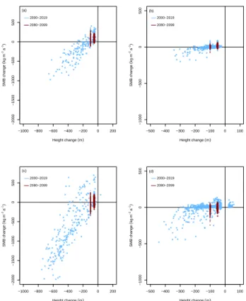
Figure 5 shows the SMB responses versus height changes for all of the perturbation experiments except NonUn t2
(re-served as a test: Sect. 2.3), divided into four partitions of SMB (negative and positive) and region (north and south of 77◦N). Each data point shows the SMB response (1Si= Sipert−Sicont) versus the height perturbation (1hi=h
pert
i −
hconti ) for a given grid cell i, so each grid cell can appear up to five times. We exclude the 906 grid cells of the NonUn t1
experiment that have | 1h |< 25 m (see Sect. 2.3). We also exclude cells in which the SMB crosses the ELA between the control and perturbed experiments (i.e. in which the per-turbed and control SMB have opposite signs) to make distinct data sets for positive and negative SMB.
Most of the variation in Fig. 5 is from the NonUn simu-lation, because this has the widest range of height perturba-tions. The south has a steeper slope, a stronger relationship between 1S and 1h, than the north.
The uniform perturbation experiments are the short verti-cal bands at 1h = (−50 m, −100 m). Most of the uniform ex-periment data in the south (bottom two subfigures of Fig. 5) show the behaviour we expect: when elevation decreases, SMB decreases (most points are in the bottom left quadrant, where both 1S and 1h are negative; 1S/1h is therefore
−1000 −800 −600 −400 −200 0 200 −2000 −1500 −1000 −500 0 500 Heightchange(m) S M B c h a n g e ( k g m − 2a − 1) ● ● ● ● ● ● ● ● ●● ● ● ● ● ● ● ● ● ● ● ● ● ● ●● ● ● ● ● ● ● ● ● ● ● ●● ●● ● ● ● ●●● ● ● ●●● ● ● ● ● ● ● ● ●● ● ● ●● ● ● ● ● ● ● ● ● ● ●● ●● ● ●● ● ● ●●● ●●● ● ● ● ● ● ● ●● ● ● ● ● ● ● ●● ● ●●●● ● ● ●●●● ● ●● ● ● ● ●●● ● ● ● ● ●●●● ● ● ● ● ● ●● ●● ● ●● ●● ●● ● ● ● ● ● ● ● ● ● ● ● ● ●● ●● ●● ● ●● ● ● ● ● ● ● ● ●●●●● ● ● ● ●● ●●● ● ● ● ●● ● ●●● ●●● ● ● ● ● ● ● ●● ●●● ●● ●● ● ●●●● ● ● ●● ●● ● ● ● ● ● ● ● ● ●●● ●●● ●● ● ● ● ● ● ● ●● ●● ● ●● ●●● ●●●●● ● ●●●●●● ● ● ● ●●● ●● ●●● ●●● ●● ●●● ●● ● ● ● ● ● ● ● ● ● ● ● ● ●● ●●● ● ●●● ●●● ●● ●● ● ● ● ● ●●● ●●● ●●● ● ●● ● ● ● ● ●● ●● ● ●● ● ●● ●●●● ● ● ●● ●● ●● ● ● ●●●● ● ● ● ● ● ● ● ●●●●● ● ●●●● ● ● ● ● ● ●●● ●●● ●●●● ●●● ● ●●● ● ● ●● ●● ● ● ● ●● ● ● ●● ●● ● ● ● ● ● ● ● ● ● ●● ●● ● ● ● ●● ● ● ● ● ● ● ● ● ●● ● ●● ●● ● ● ● ● ● ● ● ● ● ● ● ● ● ●● 2000−2019 2080−2099 (a) −500 −400 −300 −200 −100 0 100 −1000 −500 0 500 Heightchange(m) S M B c h a n g e ( k g m − 2a − 1) ●●●●●●●●●●●●●●●●●●●●●●●●●●●●●●●●●●●●●●●●●●●●●●●●●●●●●●●●●●●●●●●●●●●●●●●●●●●●●●●●●●●●●●●●●● ● ●●●●●●●●●●●●●●●●●●●●●●●●●●●●●●●●●●● ● ●●●●●●●●●●●●●●●●●●●●●●●●●●●●●●●●●●●●● ●●●●●●●●●●●●●●●●●●●●●●●●●●●●●●●●●● ● ● ●●●●●●●●●●●●●●●●●●●●●●●●●●●●●●●●● ● ● ● ●●●●●●●●●●●●●●●●●●●●●●●●●●●●●●●●● ● ●●●●●●●●●●●●●●●●●●●●●●●●●●●●●●●●● ● ● ● ●●●●●●●●●●●●●●●●●●●●●●●●●●●●●●●●●● ● ● ●● ●●●●●●●●●●●●●●●●●●●●●●●●●●●●●●●● ● ● ●●●●●●●●●●●●●●●●●●●●●●●●●●● ● ●●●●●●●●●●●●●●●●●●●●●●●●●●● ● ●●●●●●●●●●●●●●●●●●●●●●● ● ● ●●●●●●●●●●●●●●●●●●●● ● ●●●●●●●●●●●●●●●●●●● ●● ●●●●●●●●●●●●●●●●●●● ● ● ●● ● ● ●●●●●●●● ● ●●● ● ● ● ●●●●● ●●●●●● ● ●●●●●●●●●●●●●●●●●●●●●●●●●●●●●●●●●●●●●●●●●●●●●●●●●●●●●●●● ●●●●●●●●●●●●●●●●●●●●●●●●●●●●●● ● ●●●●●●●●●●●●●●●●●●●●●●●●●●●●●●● ● ● ●●●●●●●●●●●●●●●●●●●●●●●●●●●●●●● ● ●●●●●●●●●●●●●●●●●●●●●●●●●●●●●●●●●●●●●●●●●●●●●●●●●●●●●●●●●● ●●●●●●●●●●●●●●●●●●●●●●●●●●●●● ● ●● ● ●●● ●●●●●●●●●●●●●●●●●●●●● ●● ● ●●●●●●●●●●●●●●●●●●●●●● ● ● ●●●●●●●●●●●●●●●●●●● ●● ●●●●●●●●●●●●●●●●●●●●●●●●●●●●●●●●●●●● ●●●●●●●●●●●●●●●●●● ●●●●●●●●●●●●● ●● ●● ●●●●●●●● ●●●● ● ●●●●●● ● ●●●●● ● ● 2000−2019 2080−2099 (b) −1000 −800 −600 −400 −200 0 200 −2000 −1500 −1000 −500 0 500 Heightchange(m) S M B c h a n g e ( k g m − 2a − 1) ●● ● ● ● ● ● ● ● ● ●●●● ● ●● ● ●● ● ● ● ● ● ●●●●● ●● ●● ● ● ● ●● ● ● ● ● ● ●● ● ● ● ● ● ● ●● ●● ● ● ●● ● ● ● ● ●● ● ● ●● ●●● ●●●● ● ● ●●●●● ●● ● ● ● ●●● ● ● ●●●● ● ● ●●● ● ● ● ● ● ● ● ●●● ● ● ●● ●● ●●●●● ● ●● ● ● ● ● ● ● ● ●● ● ● ● ● ● ●● ● ●● ● ●●●● ● ● ● ● ● ● ● ●●● ● ● ● ●● ● ●● ● ● ● ● ● ● ● ● ● ● ● ● ●● ● ● ● ● ● ● ● ● ● ● ● ● ●●● ● ● ● ● ●●● ● ● ● ● ● ● ● ● ● ● ● ● ● ● ● ●● ● ●● ● ●● ● ●● ● ●● ●● ● ● ● ● ● ● ● ● ● ●● ●● ● ●● ● ● ● ● ● ● ● ● ● ● ● ● ●● ● ● ●● ● ● ● ● ●● ● ● ● ●● ● ● ●●● ● ● ● ● ● ● ● ● ●● ● ● ● ● ● ● ● ● ● ● ● ● ● ● ● ●● ● ● ● ●●● ●●●● ● ● ● ●●● ● ●● ● ● ●●● ● ● ● ●● ● ●●● ●●● ●● ● ●● ● ● ● ●● ●● ● ● ● ● ● ● ● ●● ● ● ● ●● ●● ● ● ● ●● ● ●●● ● ● ●● ● ● ● ● ● ● ● ● ● ● ● ● ● ●● ● ● ● ● ● ●●●● ● ● ● ● ● ● ● ●●● ● ● ● ● ●● ● ● ●● ● ●● ● ● ●● ● ●●● ● ● ● ●●● ●● ● ● ●●●●● ● ● ● ● ● ● ● ●●● ● ● ● ●●●● ●● ● ●●●● ●●● ● ● ●● ●● ● ● ● ● ● ●● ● ● ●● ● ● ● ● ●● ●●●● ●● ● ● ● ● ● ● ● ●● ● ● ● ●● ● ● ● ● ●●● ● ●● ●●●●● ● ●●●●●● ● ● ● ●●●● ● ● ● ●● ● ●● ● ●●●●● ● ●●● ●● ● ● ●●●● ● ●● ● ● ●● ● ●● ●● ● ● ● ● ● ●● ● ● ● ● ● ● ● ●● ● ●● ● ● ● ●● ● ● ● ● ● ● ● ● ● ●● ● ● ● ● ● ● ● ● ● ●● ● ● ●●●● ● ● ● ●●● ● ● ●● ● ●● ● ● ●● ●● ● ● ●●● ●● ● ● ● ● ● ● ● ●●● ●● ● ● ●● ● ● ●● ● ● ●●● ● ● ● ● ●● ● ● ● ● ●● ●●● ●● ● ● ● ● ● ●●● ● ● ●● ● ● ● ● ●● ● ●● ● ● ● ●● ●● ● ● ● ● ● ● ●● ● ● ● ● ● ● ● ● ● ●● ●● ● ● ●● ● ● ● ● ●● ●● ● ● ● ● ● ● ● ●● ● ● ● ● ● ● ● ●● ● ● ● ● ● ● ● 2000−2019 2080−2099 (c) −500 −400 −300 −200 −100 0 100 −1000 −500 0 500 Heightchange(m) S M B c h a n g e ( k g m − 2a − 1) ● ● ● ●●● ● ● ● ● ● ● ●● ● ●● ●● ● ● ● ●● ● ●● ● ●● ● ● ●●●●● ● ● ● ●●●●●● ● ● ● ●●●●●●● ● ● ● ●●●●●●●● ● ●●●●●●●●● ● ● ●● ●●●●●●●● ● ● ● ● ●●●●●●●●●● ●●●●●●●●●●●●● ● ●●●●●●●●●●● ● ●●●●●●●●●●●● ●● ●●●●●●●●●●●● ● ● ● ●●●●●●●●●●● ● ● ● ●●●●●●●●●●● ● ● ● ●●●●●●●●●●● ●●● ●●●●●●●●●●●● ● ● ● ●●●●●●●●●●●●● ●●●●●●●●●●●●●●● ● ● ● ●●●●●●●●●●●●● ● ●●●●●●●●●●●●●●● ● ● ● ●●●●●●●●●●●●● ● ● ●●●●●●●●●●●●●●● ●● ●●● ● ●●●●●●●●●●●●●●●●●●●●● ● ●●●●●●●●●●●●●●●●●●●●●● ●●●●●●●●●●●●●●●●●●●● ● ● ●●●●●●●●●●●●●●●●●●●● ●●● ●●●●●●●●●●●●●●●●●●●●● ● ●●●●●●●●●●●●●●●●●●●●● ●●●●●●●●●●●●●●●●●●●●●●● ●●● ●●●●●●●●●●●●●●●●●●●●●●●●●●●●●●●●●●●●●●●●●● ● ●●●●●●●●●●●●●●●●●●●●● ●● ●●● ●●●●●●●●●●●●●●●●●●●●●●●●●●●●●●●●●●●●●●●●●●●●●●●●●●●●●●● ●●●● ● ●●●●●●●●●●●●●●●●●●●●●●●●●●●●●●● ● ●●●●●●●●●●●●●●●●●●●●●●●●●●●●●●●●●●●●●●●●●●●●●●●●●●●●●●●●●●●● ●●● ● ●●● ●●●●●●●●●●●●●●●●●●●●●●●●●●●● ● ●●●●●●●●●●●●●●●●●●●●●●●●●●●● ● ●●●●●●●●●●●●●●●●●●●●●●●●●●●●●●●●●●●●●●●●●●●●●●●●●●●●●●●●●●●●●●●●●●●●●●●●●●●●●●●●●●●●●●●● ● ●●●●●●●●●●●●●●●●●●●●●●●●●●●●● ● ●●●●●●●●●●●●●●●●●●●●●●●●●●●●● ●●●●●●●●●●●●●●●●●●●●●●●●●●●● ●● ●●●●●●●●●●●●●●●●●●●●●●●●●●●● ● ●●●●●●●●●●●●●●●●●●●●●●●●●●●●●●● ●●●●●●●●●●●●●●●●●●●●●●●●●●●●●●●● ● ● ●●●●●●●●●●●●●●●●●●●●●●●●●●●●●●●●●●●●●●●●●●●●●●●●●●●●●●●●●●●●● ● ●●●●●●●●●●●●●●●●●●●●●●●●●●●●●● ● ●●●●●●●●●●●●●●●●●●●●●●●●●●●●● ● ●●●●●●●●●●●●●●●●●●●●●●●●●●●●●● ● ●●●●●●●●●●●●●●●●●●●●●●●●●●●●●● ●●●●●●●●●●●●●●●●●●●●●●●●●●●●●●●●●●●●●●●●●●●●●●●●●●●●●●●●●●●●●● ● ● ●●●●●●●●●●●●●●●●●●●●●●●●●●●●●●● ● ●●●●●●●●●●●●●●●●●●●●●●●●●●●●●●●● ● ●●●●●●●●●●●●●●●●●●●●●●●●●●●●●●●●● ●●●●●●●●●●●●●●●●●●●●●●●●●●●●●●●●●●●● ● ● ●●●●●●●●●●●●●●●●●●●●●●●●●●●●●●●●●●●● ●●●●●●●●●●●●●●●●●●●●●●●●●●●●●●●●●●●● ● ●●●●●●●●●●●●●●●●●●●●●●●●●●●●●●●●●●●● ● ●●●●●●●●●●●●●●●●●●●●●●●●●●●●●●●●●●●●●●●●●●●●●●●●●●●●●●●●●●●●●●●●●●●● ● ●●●●●●●●●●●●●●●●●●●●●●●●●●●●●●●●● ● ● ●●●●●●●●●●●●●●●●●●●●●●●●●●●● ● ●● ●●●●●●●●●● ● ● ●●●●● ●● ●●●● ● ●●● ●● ● ●● ● ● ● ● ● ●● ● ●● ● ● ●● ● ● ● ● ●●● ● ● ● ● ●●● ● ●● ● ●●●●● ● ● ● ● ●●●● ● ● ●● ● ●●●●●● ● ● ● ●●●●●● ● ●● ● ●●●●●●●● ● ● ● ● ●●●●●●● ● ● ● ●●●●● ●● ● ● ● ● ●●●●●●● ● ● ● ●●●●●● ● ●● ● ● ●●●●●●●● ● ● ● ●●●●●●●● ● ● ● ● ●●●●●● ● ● ● ● ●●●●●●● ●● ●● ●●●●●●● ● ●● ●●●●●●●● ● ● ● ● ● ●●●●●●●● ●● ● ● ●●●●●●●●● ● ● ● ●●●●●●●●●● ● ● ●●●●●●●●●●● ●● ●●●●●●●●●● ● ●● ●●●● ● ●●●●●●●●●●●●●●●●● ● ●●● ●●●●●●●●●●●●●●● ● ●● ●●●●●●●●●●●●●●●●● ● ● ●●●●●●●●●●●●●●●● ● ● ● ●●●●●●●●●●●●●●●●● ● ●●●●●●●●●●●●●●●●●● ● ●●●●●●●●●●●●●●●●● ●●● ●●●●●●●●●●●●●●●●●● ●●●●●●●●●●●●●●●●● ● ●●●●●●●●●●●●●●●●● ● ● ●●●●● ● ●●●●●●●●●●●●●●●●●●●●●●● ●●● ●● ●●●●●●●●●●●●●●●●●●●●●●●●●●●● ● ● ●●●●●●●●●●●●●●●●●●●●●●● ●●● ●● ● ● ●●●●●●●●●●●●●●●●●●●●●●● ● ● ● ● ●● ●●●●●●●●●●●●●●●●●●●●●●●● ● ● ●● ●●●●●●●●●●●●●●●●●●●●●●●● ●●●●●●●●●●●●●●●●●●●●●●●●●● ● ●●●●●●●●●●●●●●●●●●●●●●●●● ● ●●●●●●●●●●●●●●●●●●●●●●●●●●●●●●●●●●●●●●●●●●●●●●●●●● ●●●●●●●●●●●●●●●●●●●●●●●●●●● ● ●●●●●●●●●●●●●●●●●●●●●●●● ● ● ●●●●●●●●●●●●●●●●●●●●●●●●●●●●●●●●●●●●●●●●●●●●●●●●●●●●●● ● ●●●●●●●●●●●●●●●●●●●●●●●●●●●● ● ●●●●●●●●●●●●●●●●●●●●●●●●●●●●●●●●●●●●●●●●●●●●●●●●●●●●●●● ●● ●●●●●●●●●●●●●●●●●●●●●●●●● ● ● ● ●●●●●●●●●●●●●●●●●●●●●●●●●● ● ●●●●●●●●●●●●●●●●●●●●●●●●●● ● ● ●●●●●●●●●●●●●●●●●●●●●●●●●● ● ● ●●●●●●●●●●●●●●●●●●●●●●●●●●● ● ●●●●●●●●●●●●●●●●●●●●●●●●●●● ● ● ●●●●●●●●●●●●●●●●●●●●●●●●●●●● ● ●●●●●●●●●●●●●●●●●●●●●●●●●●●● ● ● ●●●●●●●●●●●●●●●●●●●●●●●●●●●●● ●●●●●●●●●●●●●●●●●●●●●●●●●●●●●●●● ● ● ●●●●●●●●●●●●●●●●●●●●●●●●●●●●●●●● ● ●●●●●●●●●●●●●●●●●●●●●●●●●●●●●●●●● ● ●●●●●●●●●●●●●●●●●●●●●●●●●●●●● ●●● ●●●●●●●●●●●●●●●●●●●●●●●●●●●●● ●● ● ●●●●●●●●●●●●●●●●●●●●●●●●●●●●●● ● ●●●●●●●●●●●●●●●●●●●●●●●●●●●●● ●●●●●●●●●●●●●●●●●●●●●●●●●●●● ●● ●●●●●●● ● ●●●● ● ●● ● 2000−2019 2080−2099 (d)
Fig. 5. Scatter plots of SMB change ∆S versus height change ∆h for grid cells north (top row) and south (bottom) of 77◦N, divided into grid cells with SMB in both the control and perturbed experiments less than zero (left column) and greater than or equal to zero (right). Data with height change | ∆h | < 25 m
are excluded. 34
Fig. 5. Scatter plots of SMB change 1S versus height change 1h
for grid cells north (top row) and south (bottom) of 77◦N, divided into grid cells with SMB in both the control and perturbed experi-ments less than zero (left column) and greater than or equal to zero (right). Data with height change | 1h | < 25 m are excluded.
positively signed). But in the north (top two subfigures), the response is the opposite: when elevation decreases, SMB in-creases (most points are in the top left quadrant, with posi-tive 1S and negaposi-tive 1h; 1S/1h is negaposi-tive). This change in response from north to south can be seen in the maps in Fig. 3, particularly for the −100 m experiment (top two sub-figures) where the SMB change along the margin is positive (red) north of 77◦N and mostly negative (blue) in the south. However, most of the uniform experiment data do lie within the range of the NonUn results.
2.2 Parameterisation structure
The parameterisation comprises four “SMB lapse rates”, gra-dients that characterise a linear relationship between SMB change and surface elevation change. When testing the pa-rameterisation, we use the gradients to adjust the control SMB using the NonUn height changes and compare with the actual NonUn SMB results. In a companion paper we use the parameterisation with several ice sheet models to dynamically adjust projections of future SMB as the GrIS shape evolves (Edwards et al., 2014). The four gradients cor-respond to the four possible combinations of the grid cell adjusted mean SMB over the past decade being positive or
negative and the grid cell latitude being north or south of 77◦N. We estimate these gradients from the ratios of SMB
changes to height changes (1S/1h) in the surface elevation perturbation experiments. This parameterisation structure is determined by a combination of a priori choices and informal tests.
We choose the structure of our parameterisation with the following aims: to preserve as much of the SMB–elevation relationship in the MAR simulations as possible; to use as few assumptions as possible; to be applicable to any SMB forcing from MAR; and to be simple for the ice sheet mod-eller to implement. We test the ability of the parameterisation to reproduce the SMB field in the NonUn t2simulation when
applied to the control t2simulation using the NonUn height
changes.
We parameterise the relationship between elevation and mean SMB, using total SMB rather than its individual com-ponents (as in Franco et al., 2012) so it is easier to implement in ISMs and requires only one simulated variable as the input forcing. We also choose to parameterise changes in SMB as a function of changes in elevation (in common with Franco et al., 2012), rather than absolute values (as in Helsen et al., 2011). If we were to parameterise the relationship between absolute SMB S and absolute height h, using a linear model
S = a + bh(e.g. in Fig. 4), we would force the adjusted SMB
to lie along a single line lying somewhere between the data from the two time periods t1and t2, with large uncertainty
in the intercept due to the climate dependence of SMB at a given height. Instead, we can parameterise the relationship between SMB changes and height changes, 1S = b1h, esti-mating only the gradient b. This way SMB can be adjusted up or down the slope apparent in the data, rather than onto a single line with constant intercept. Eliminating the intercept in this way preserves the climate dependence of the SMB– elevation relationship in the MAR simulations, and removes half the unknown parameters. Working with anomalies rather than absolute values is also a standard approach in climate modelling, because the former are thought to be simulated more reliably than the latter.
The adjusted SMB is Sadj=SRCM+b1h, where SRCM is the original SMB (kg m−2a−1), 1h the height change (m), and b the SMB–elevation gradient b = 1S/1h (kg m−3a−1). More specifically, for a given MAR grid cell in a year t a gradient bt is used to adjust the control SMB StRCM using the height difference between the NonUn and control experiments, Stadj=StRCM+bt(hNonUn−hcont). The
gradient btis selected according to the “reference” SMB and
latitude of the grid cell, where the reference is the mean of the adjusted SMB over the previous 10 yr (see Edwards et al., 2014, for more details). Using the adjusted SMB for the ref-erence means the gradient selection evolves as part of the feedback, which helps to make the method more robust with changing climate.
Our height perturbation simulations allow us to derive the gradients directly from SMB responses to height changes for each grid cell, rather than the difference in SMB between grid cells in different locations on the ice sheet (as in Helsen et al., 2011). This is important because the SMB response may be determined by different physical processes due to local topography and atmospheric circulation patterns. Each grid cell i provides an estimate of the gradient b = 1S/1h from the SMB change (perturbed SMB minus control SMB,
1Si=S
pert
i −Sicont) versus the elevation change (perturbed
height minus control height, 1hi=h
pert
i −hconti ). In Fig. 4
these correspond to the arrow slopes; in Fig. 5 they are the
yaxis values divided by the x axis values.
We choose not to make the gradients a function of grid cell location (Helsen et al., 2011; Franco et al., 2012), other than the north–south divide, to avoid dependence on the MAR grid resolution (Franco et al., 2012) and make the isation as generic as possible. A spatially varying parameter-isation would be tailored to the current shape of the ice sheet and the gradients would need to be interpolated for the ISM grid, which could lead to distorting edge effects at discon-tinuities such as the margin, ELA, and grid cell boundaries (e.g. Franco et al., 2012).
We do not make the gradients a function of climate or time (beginning versus end of the century), because this would restrict our ability to apply the parameterisation to other MAR simulations: for the missing years of the A1B scenario (2020–2079) we could interpolate or otherwise scale the re-sults, but this would be less reliable or applicable for other emissions scenarios and simulations forced by other GCMs. To guide our choices for other aspects of the parameterisa-tion structure, we consider various methods of estimating and applying the gradients and quantify their relative success in reproducing SMB changes in one of the perturbation exper-iments. We estimate the gradients from the SMB responses in the two NonUn simulations, then use them to adjust the SMB in the control t2 experiment according to the NonUn
height changes. We quantify success by comparing the pa-rameterised cumulative SMB change with the actual results in the NonUn t2simulation, in terms of both the root mean
square error in the spatial pattern and the error in the GrIS total (not shown). We base our decisions on a combination of practical considerations (such as ease of implementation) and these informal sensitivity tests, rather than a systematic optimisation across all possible choices.
Our final gradients are a function of SMB sign (posi-tive/negative) and region (north/south), because these divi-sions make substantial improvements to the parameterisation while not introducing much complexity when implement-ing in ISMs. The clear difference in SMB response above and below the ELA has already been discussed (Sect. 2.1). We also choose to divide by region because of the distinct regimes in Fig. 4 in which the north has a shallower gradi-ent and larger intercept than the south. The uniform height
change simulations also indicate that the the northern mar-gin behaves differently (Fig. 3). We test the performance of north–south divisions in half degree intervals in the range 74–79◦N, and also compare with using no division, and find that 77◦N gives the best result.
We test two other functional dependencies for the gradi-ents: eight divisions in SMB rather than two, and height de-pendence as well as SMB dede-pendence. The improvements are not marked enough to justify the extra complexity.
We try three methods for estimating gradients: (a) a lin-ear model of S versus h, (b) a linlin-ear model of 1S versus
1h with zero intercept, and (c) a non-parametric method. We apply each to the four data sets (positive/negative SMB, north/south), and grid cells with | 1h | < 25 m are excluded. In method (a), a linear fit of S vs. h estimates the gradi-ent b in Fig. 4; this is a similar approach to Helsen et al. (2011), except that we then make the SMB adjustment with our anomaly method rather than an intercept. In method (b), a linear fit of 1S versus 1h estimates the gradient b in Fig. 5; a zero intercept reflects our expectation that mean SMB change is zero if there is no height change. In method (c), we use a non-parametric approach instead of a linear model. This takes the median of 1S / 1h ratios (y/x in Fig. 5) as an es-timate of b. Method (a) is the least successful, and (b) is the most successful. But we judge that (b) is not an appropri-ate method, because the fit residuals for grid cells above the ELA vary systematically as a function of height change. Part of this may be due to our constraint of a zero intercept, but the data also clearly have non-linear structure (Fig. 5). The non-parametric method avoids model assumptions such as normally distributed fit residuals, allowing us to capture all the aspects of the MAR response. Our final method is there-fore based on (c), though we use the full distribution rather than the median (Sect. 2.3).
Our final parameterisation of the SMB–elevation feedback is therefore a set of four gradients, b = (bNp, bNn, bpS, bSn), that are used to adjust SMB with a linear model of SMB change versus elevation change. A gradient is selected from the set of four according to whether the mean of the adjusted SMB in the previous decade is positive (p) or negative (n) and whether the grid cell is north or south of 77◦N (N, S). The gradients are estimated from the ratios 1S/1h of grid cells in the MAR perturbation experiments.
The full SMB–elevation relationship is complex, but our aim is to create a parameterisation that is straightforward to implement: we have therefore partially linearised it, by par-titioning the data four ways and by using a linear model of SMB adjustment. In the following section our aim is to ac-count for this approximation with non-parametric assessment of uncertainties in those linear parameters. With this struc-ture it is easy to implement the parameterisation, to use it in forcing an ice sheet model, and to assess the impacts of the parametric uncertainty (arising in large part from this lineari-sation) using additional ice sheet model simulations.
2.3 Parameter estimation
We now turn to formal statistical inference to obtain the fi-nal gradient values. We wish to assess the full uncertainty in the SMB–elevation relationship rather than using only tuned (“best estimate”) values or performing ad hoc sensi-tivity tests. This is particularly important given there are op-posite sign SMB responses to elevation changes in the simu-lations. So we estimate full probability distributions for each of the four gradients (b = bNp, bNn, bpS, bSn) using a Bayesian approach. This also allows us to propagate the probabilis-tic SMB–elevation feedback uncertainty to predictions of the GrIS contribution to sea level (Edwards et al., 2014).
We derive initial (“prior”) distributions for the four gradi-ents using SMB responses from five of the six perturbation simulations: −100 m, t1and t2; −50 m, t1and t2; and NonUn
t1. These five experiments thus include parameter estimates
under different climates (t1and t2), different height changes
(−50 m, −100 m, and NonUn), and different locations for a uniform height change (−50 m, −100 m).
We reserve the final simulation (NonUn t2) as a test of
the parameterisation, reweighting the prior distributions us-ing the degree of success in reproducus-ing the cumulative sea level change to obtain updated (“posterior”) distributions. We choose NonUn t2because the NonUn height changes span a
wider range and are closer in spatial pattern to those expected in a warmer climate than the uniform height changes, and be-cause the SMB signal is larger for t2than for t1; we are more
concerned that the parameterisation is valid under a warmer climate than the present day.
This division of simulations allows us to try a wide range of candidates for parameter values but assign larger weights to those that match the target we wish to reproduce: the ag-gregate behaviour of the whole ice sheet.
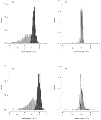
We use histograms of the ratio of SMB changes to height changes, 1S / 1h (Fig. 6), as a basis for our prior distribu-tions for the four linear gradient values. These are the same data as in Fig. 5, which shows 1S versus 1h. Our mini-mum threshold for the denominator, | 1h |≥ 25 m, removes extreme values from the tails of these distributions which sta-bilises estimation of the ratios. All four distributions show that SMB is sometimes positively correlated with height, sometimes negatively correlated. Above the ELA (Figs. 6b and d) the histograms for bNp and bSp are very narrow: the SMB responses for a given height change are small in magni-tude with little variation. Below the ELA (Figs. 6a and c) the histograms for bNn, bnS are much broader, showing the wide variation in response for different regions of the ice sheet. These histograms are dominated by the four uniform pertur-bation simulations.
Each of the four histograms has a different number of grid cells, so we take equally sized subsets of each to obtain a joint sample of the gradient set b: for each histogram we order the values of 1S / 1h and take the 0.5 % to 99.5 % quantile val-ues in 0.5 % steps, giving 199 samples of the four gradients
SMBchange heightchange(kgm−3a−1) Frequency −10 −5 0 5 10 0 50 100 150 200 (a)
SMBchange heightchange(kgm−3a−1)
Frequency −10 −5 0 5 10 0 500 1000 1500 2000 (b)
SMBchange heightchange(kgm−3a−1)
Frequency −10 −5 0 5 10 0 100 200 300 400 (c)
SMBchange heightchange(kgm−3a−1)
Frequency −10 −5 0 5 10 0 2000 4000 6000 (d)
Fig. 6. Histograms of the ratio ∆S/∆h for grid cells north (top row) and south (bottom) of 77◦N, divided into grid cells with SMB in both the control and perturbed experiments less than zero (left column) and greater than or equal to zero (right). Data with height change | ∆h | < 25 m are excluded.35
Fig. 6. Histograms of the ratio 1S/1h for grid cells north (top row)
and south (bottom) of 77◦N, divided into grid cells with SMB in both the control and perturbed experiments less than zero (left col-umn) and greater than or equal to zero (right). Data with height change | 1h | < 25 m are excluded.
(bNp, bNn, bSp, bnS). These prior distributions are shown in light grey in Fig. 7.
We use each of these 199 prior estimates of the gradient set to adjust the control SMB in 2080–2099 according to the NonUn height change, and assess their success in reproduc-ing the target NonUn t2experiment. Each gradient set is used
to calculate a spatial pattern of cumulative SMB change and the corresponding total GrIS cumulative sea level contribu-tion.
We simplify the statistical modelling by choosing com-parisons so that the differences (discrepancies) between the adjusted and target SMB at each location are approximately i.i.d. (independent and identically distributed) in space. We make the comparisons approximately independent by “thin-ning” (Rougier and Beven, 2013), using only every 5th grid cell (125 km spacing). This spacing removes spatial corre-lation: an empirical variogram of the thinned discrepancies is flat for all lengths up to around 800 km (the width of the ice sheet). We assume the discrepancies are identically dis-tributed in space, that is, that the model is equally likely to match the target at every location. We also assume that the discrepancies are normally distributed. In the absence of fur-ther information and as a first attempt to describe parameter-isation uncertainty, these choices and assumptions allow us
Gradient (kg m−3 a−1) Density −6 −4 −2 0 2 4 0.0 0.5 1.0 1.5 (a) Gradient (kg m−3 a−1) Density −2 −1 0 1 2 0 2 4 6 8 (b) Gradient (kg m−3 a−1) Density −6 −4 −2 0 2 4 0.0 0.5 1.0 1.5 (c) Gradient (kg m−3 a−1) Density −2 −1 0 1 2 0 2 4 6 8 (d)
Fig. 7. Prior (light grey) and posterior (dark grey) distributions of the four value gradient set, b = (bN
p,bNn,bSp,bSn) for regions north (bN, top row) and south (bS, bottom) of 77
◦N, and SMB less than zero (bn, left column) and greater than or equal to zero (b36p, right).
Fig. 7. Prior (light grey) and posterior (dark grey) distributions of
the four value gradient set, b = (bNp, bNn, bSp, bSn)for regions north (bN, top row) and south (bS, bottom) of 77◦N, and SMB less than zero (bn, left column) and greater than or equal to zero (bp, right).
to avoid the difficult task of modelling the spatial correlation and variation of the discrepancies.
These assumptions translate to a simple metric for assess-ing the gradient estimates. The scorassess-ing, “likelihood”, func-tion is a multivariate (for multiple locafunc-tions) independent Gaussian with constant variance; the exponent is the sum of squared differences between the adjusted SMB and the target SMB over the subsampled grid cells (independent: a prod-uct of Gaussians) divided by the “discrepancy variance” σ2 (identically distributed: constant variance). The multiplica-tive constant is discarded due to normalisation later. So the score sj for the j th of 199 samples of b is
sj=exp " −1 2σ2 X i (fij−zi)2 # , (1)
where f is the adjusted SMB, z the target SMB, and i the grid cell index. The discrepancy variance is a parameter that represents how closely we expect the parameterised SMB to match the target; our choice is discussed below.
The weight given to each gradient set is the normalised score, wj=sj/P
j
sj. Note that a single weight is
calcu-lated for each gradient set b, rather than individual weights for each of the four components. The most successful
Table 1. The 2.5 % quantile, best estimate, and 97.5 % quantile
estimates of the SMB–elevation gradients in kg m−3a−1, below (SMB < 0) and above (SMB ≥ 0) the ELA, for regions north and south of 77◦N.
Region 2.5 % Best estimate 97.5 % SMB < 0 North −0.22 0.56 1.33
South 1.03 1.91 2.61
SMB ≥ 0 North −0.03 0.09 0.23
South −0.07 0.07 0.59
(“maximum likelihood”) gradient set ˜b has the smallest sum
of squared differences and therefore the largest weight. We calculate posterior distributions for the four components of
b by reweighting the prior distributions with the normalised
weights. We estimate probability densities from the his-tograms with kernel density estimates and use these to es-timate the modes of the posterior distributions, which are our best estimates of the gradients. As we are in a Bayesian framework, our uncertainties are expressed as “credibility in-tervals” rather than confidence intervals. We estimate 95 % credibility intervals with bootstrapping: we resample 100 000 times from the 199 gradient values (with replacement, using the normalised weights), smooth these with the same band-width, and estimate the 2.5 % and 97.5 % quantiles.
Our statistical framework requires minimal choices: the form of the likelihood function; the spacing for the sub-sampling; and a value for the discrepancy variance. We also choose to set the bandwidth (standard deviation of the smoothing) for the kernel density estimation because the au-tomatically chosen value (Silverman, 1986) does not seem to adequately resolve the distribution shapes. We test var-ious options and make our final choices with the follow-ing considerations: thinnfollow-ing so that the discrepancies appear approximately uncorrelated in space; the variance σ2 cho-sen such that the weights are not concentrated on a small number of gradient estimates and most or all of the dis-crepancies for the maximum likelihood parameterisation ( ˜b)
are in the range ±3σ (Pukelsheim, 1994); and the posterior distribution of total GrIS sea level contribution is close to the target. We choose the smoothing bandwidth so that the density profile captures the main features of the histogram. Our final choices are a Gaussian likelihood function; sub-sampling distance 5 grid cells (125 km); discrepancy vari-ance σ2=(20 × 103Gt)2; and bandwidths 0.15 kg m−3a−1 for gradients below the ELA and 0.05 kg m−3a−1above the ELA. Sensitivity tests for these choices are described in the next section.
2.4 Results
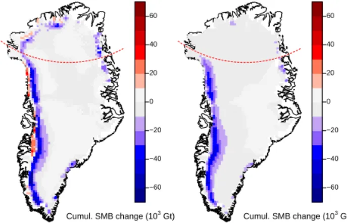
Figure 8 shows the adjusted cumulative SMB from the max-imum likelihood parameterisation ( ˜b) and the target. The
maximum likelihood gradient set reproduces the target well
Cumul. SMB change (103 Gt) −60 −40 −20 0 20 40 60 Cumul. SMB change (103 Gt) −60 −40 −20 0 20 40 60
Fig. 8. Cumulative SMB change at the end of the NonUn 2080–2099 simulation: (left) target MAR simulation (perturbed minus control) and (right) result from maximum likelihood gradient set ˜b applied to the NonUn height change (adjusted minus control). Red dashed line is 77◦N.
37
Fig. 8. Cumulative SMB change at the end of the NonUn 2080–
2099 simulation: (left) target MAR simulation (perturbed minus control) and (right) result from maximum likelihood gradient set ˜b
applied to the NonUn height change (adjusted minus control). Red dashed line is 77◦N.
in most areas, but cannot reproduce the SMB increases with decreasing elevation along the western and southeastern ice sheet margins. Figure 9 shows the discrepancies between the two for all grid cells and the subset used for the likelihood calculation. Most of the discrepancies are small over the ice sheet interior and larger at the margin.
Figure 7 shows the posterior distributions (dark grey) for the four gradients; Table 1 gives the best estimates and 95 % credibility intervals. The posterior distributions are mostly positive, with much larger gradients below the ELA, par-ticularly in the south, than above. Most of the distributions are fairly symmetric, except the south above the ELA which has a low best estimate and a long tail of larger values. The weighting has a particularly strong effect for grid cells be-low the ELA, drastically narrowing the distributions: effec-tively the likelihood scoring gives high weights to the gra-dient estimates derived from the NonUn 2000–2019 experi-ment (large, positive values), rather than the uniform height change experiments (small, positive and negative values), be-cause these are most successful in reproducing the patterns of change in the NonUn 2080–2099 experiment.
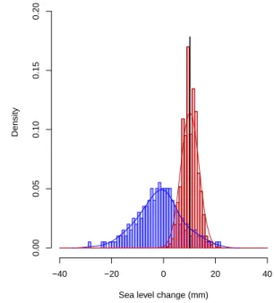
We can apply the same weights to the total GrIS cumula-tive sea level contributions for each sample of the gradient set (Fig. 10). The prior distribution is centred close to zero: the prior estimate of the elevation feedback is that it has no net effect. The update narrows and shifts the posterior distribu-tion so that it is centred on the target, a positive contribudistribu-tion from the feedback.
We test the sensitivity of the results to the elevation thresh-old and statistical modelling choices. Varying the threshthresh-old (from the default 25 m) between 10 m and 50 m in 5 m in-tervals changes the results by no more than 0.02 kg m−3a−1, and in most cases 0.01 kg m−3a−1or zero, for the majority of the gradient best estimates and CI bounds. The exceptions are the best estimates in the south (bnS, bSp) and the upper CI
Cumul. SMB change (103 Gt) −60 −40 −20 0 20 40 60 Cumul. SMB change (103 Gt) −60 −40 −20 0 20 40 60
Fig. 9. Cumulative SMB change at the end of the NonUn 2080–2099 simulation: (left) error in the maximum likelihood gradient set ˜b applied to the NonUn height change (adjusted minus perturbed), and (right) the subset of those grid cells used in the calculation of the weights (discrepancies fij− ziin
Eq. 2.3). Red dashed line is 77◦N.
38
Fig. 9. Cumulative SMB change at the end of the NonUn 2080–
2099 simulation: (left) error in the maximum likelihood gradient set
˜
b applied to the NonUn height change (adjusted minus perturbed),
and (right) the subset of those grid cells used in the calculation of the weights (discrepancies fij−zi in Eq. 1). Red dashed line is
77◦N.
bound for the latter (bSp), where the changes are in the range 0.06–0.12 kg m−3a−1. These correspond to a 5 % change for
bSn; for the smaller gradient bpS the fractional changes are larger, but the changes plateau (i.e. the gradient estimates sta-bilise) above 25–30 m, as intended with the use of the thresh-old.
We try substituting the Gaussian likelihood with a Cauchy (Student’s t distribution with one degree of freedom; very heavy tailed), scaled to match a Gaussian at the 25 % and 75 % quantiles. Our motivation is that the histogram of dis-crepancies for the maximum likelihood gradient set is fairly sharply peaked. The effect of a Cauchy likelihood is to dis-tribute the weights over a much smaller number of gradient sets, which drastically narrows the posterior distributions. If we also reduce the bandwidths to match these narrower distributions (from 0.15 to 0.05 kg m−3a−1below the ELA and from 0.05 to 0.03 kg m−3a−1above), the CI widths de-crease by 54–84 %, and the best estimates inde-crease by 13– 38 % for three of the gradients and 186 % (from 0.07 to 0.20 kg m−3a−1) for bpS. Because the weights are so concen-trated, and we wish to be conservative with uncertainty es-timates, we choose the Gaussian likelihood. An alternative approach would be to set a larger discrepancy variance for the ice sheet margin grid cells than the interior, though one might be less confident in assigning the value of two uncer-tain parameters rather than one.
The discrepancies for the maximum likelihood parameter-isation are all within ±1.5σ , which indicates that our dis-crepancy variance is too large; on the other hand, reducing σ concentrates the weights on a smaller number of gradient es-timates, leading to narrower posterior distributions and 95 % CIs. Changing σ from 20 to 15 or 25 Gt does not affect the best estimates much (0–11 %) except for the small-valued bSp (43 %). Increasing or decreasing σ by 5 Gt has the effect of
Sea level change (mm)
Density −40 −20 0 20 40 0.00 0.05 0.10 0.15 0.20
Fig. 10. Prior (blue) and posterior (red) distributions of cumulative change in sea level at 2099 using parameterised elevation feedback for height changes in the NonUn simulation. The target is the result from the NonUn 2080–2099 experiment (vertical black line).
39
Fig. 10. Prior (blue) and posterior (red) distributions of cumulative
change in sea level at 2099 using parameterised elevation feedback for height changes in the NonUn simulation. The target is the result from the NonUn 2080–2099 experiment (vertical black line).
increasing or decreasing the CI widths by 12–24 %. Decreas-ing σ to 15 or 10 Gt broadens the discrepancies to about 2σ , but concentrates the weights rather more. Again, we err on the side of conservatism in our choice.
In the grid cell sampling (required for independence), us-ing different spacus-ing does not have a monotonic effect on the results. Decreasing the spacing from 5 grid cells to 4 (100 km) or increasing it to 6 (150 km) both have the effect of decreasing most best estimates and CI widths. This in-dicates it is not a problem of using too short a correlation length (violating the independence assumption) but of sensi-tivity to the grid cell sampling, most likely at the ice sheet margin. Of these three choices, the 5 cell spacing produces the best match to the cumulative sea level change in Fig. 10; in other words, both the 4 and 6 cell spacings concentrate the weights on smaller gradients (smaller SMB adjustments), which match the target spatial pattern well for the particular sampled cells but perform poorly for the ice sheet total us-ing all grid cells. We alter the offset of the samplus-ing, which also has a non-monotonic effect. Shifting both the longitudi-nal and latitudilongitudi-nal offsets by −3 cells gives a small decrease in the best estimate (0 to −4 %), while offsets of −2, −1 and +1 all give higher best estimates (15–34 %, except bSp 71–100 %). The effect on CI width is also mixed; the largest effect is on bSp, up to 26 %.
Using a larger discrepancy variance for the margin than the interior would reduce the sensitivity of the results to sam-pling, because the margin grid cells would have less effect on the likelihood value.