HAL Id: halshs-01828643
https://halshs.archives-ouvertes.fr/halshs-01828643
Preprint submitted on 3 Jul 2018HAL is a multi-disciplinary open access archive for the deposit and dissemination of sci-entific research documents, whether they are pub-lished or not. The documents may come from teaching and research institutions in France or abroad, or from public or private research centers.
L’archive ouverte pluridisciplinaire HAL, est destinée au dépôt et à la diffusion de documents scientifiques de niveau recherche, publiés ou non, émanant des établissements d’enseignement et de recherche français ou étrangers, des laboratoires publics ou privés.
Assessing competition on Maritime Routes in the Liner
Shipping Industry through multivariate analysis
Nikola Kutin, Patrice Guillotreau, Thomas Vallée
To cite this version:
Nikola Kutin, Patrice Guillotreau, Thomas Vallée. Assessing competition on Maritime Routes in the Liner Shipping Industry through multivariate analysis. 2018. �halshs-01828643�
EA 4272
Assessing competition on Maritime
Routes in the Liner Shipping Industry
through multivariate analysis
Nikola Kutin*,**
Patrice Guillotreau*
Thomas Vallée*
2018/09
(*) LEMNA - Université de Nantes
(**) National University of Management (Cambodge)
Laboratoire d’Economie et de Management Nantes-Atlantique Université de Nantes
Chemin de la Censive du Tertre – BP 52231 44322 Nantes cedex 3 – France http://www.lemna.univ-nantes.fr/ Tél. +33 (0)2 40 14 17 17 – Fax +33 (0)2 40 14 17 49
Docum
ent
de Tra
vai
l
W
or
ki
ng P
ape
r
1
Assessing competition on Maritime Routes in the Liner Shipping Industry
through multivariate analysis
Nikola KUTINa, Patrice GUILLOTREAUb and Thomas VALLEEc
a. LEMNA, University of Nantes (France) and National University of Management (Cambodia), Chemin de la Censive du Tertre, Bâtiment Erdre, 44322 Nantes,
nikola.kutin@etu.univ-nantes.fr, nikola.kutin@num.edu.kh.
b. LEMNA, University of Nantes (France), Chemin de la Censive du Tertre, Bâtiment Erdre, 44322 Nantes, patrice.guillotreau @univ-nantes.fr
c. LEMNA, University of Nantes (France), Chemin de la Censive du Tertre, Bâtiment Erdre, 44322 Nantes, thomas.vallee@univ-nantes.fr
Abstract
The current paper investigates the level of competition on maritime routes in the liner shipping industry by applying multivariate and cluster analyses on maritime indicators. We use a dataset which includes maritime routes between 153 ports for the year 2014, described by several characteristics regarding the number of operators, the number of ships and trips, the size of ships, the sea distance, the bilateral countries’ connectivity. Some clusters of maritime routes are identified along two key components, a first one related to the number of competing firms, and a second one where the average size of firms is positively correlated with distance. The first one indicates somehow the degree of competition while the second one is related to the efficiency of carriers. Another way of looking at competition is to consider the region-based trade and to see whether indicators respond differently from region to region.
2
This work was supported by the European Union’s Erasmus+ Programme, Key Action 2, Capacity building in the field of higher education under DOCKSIDE Project (www.dockside-kh.eu), Grant number: 573790-EPP-1-2016-1-FR-EPPKA2-CBHE-SP.
1. Introduction
Since the invention of the shipping container by Malcolm McLean in 1956, the containerized trade has experienced a remarkable growth. It allowed port operators and shipping carriers to reduce their loading and unloading costs and to considerably improve their time efficiency. According to Clarkson Research’s data, since 1990, the container trade has increased by more than 600%. In 2016, it accounted for only 16.7% of the total seaborne trade, while its value was more than 60%1. In the last decades, we have observed a specialization of the ports by investing
in the construction and enlargement of container terminals and connections with the hinterland network. Major investments, such as the $8.2 billion expansion program of the Suez Canal completed in July 20152 and the enlargement of the Panama Canal for $5.25 billion
achieved in June 2016, made faster and cheaper the operation of large container vessels.
From 1999 to 2016, the average size of containerships and the volume of containerized cargo per mile has increased by 127% and 208%3, respectively. This positive trend is largely driven by
the rapid pace of globalization which was amplified by the inclusion of China in the WTO membership in December 2001. As a consequence of globalization, the prevailing network structure in the maritime trade has turned into a “hub and spoke” structure. Some ports, such as Hong Kong and Singapore, located on central strategic geographical sites (hubs) have direct connections with regional ports (feeders or spokes) and other hub ports.
Along this hub and spoke network organization, the liner shipping industry has been rapidly developed by exploiting large increasing returns to scale, through which the most transited
1http://www.worldshipping.org/about-the-industry/global-trade
2https://www.economist.com/news/middle-east-and-africa/21660555-it-necessary-bigger-better-suez-canal
3
routes are covered by the largest ships, having a high loading factor and organized within alliances (Yang et al., 2011). Such a growing average size of ships on a few major routes linking port hubs has reduced the number of liner companies after several waves of mergers & acquisitions (Clark et al., 2004). For market leaders, such an external growth strategy represents a way of defending their positions and increasing entry barriers, like the recent Maersk Line’s acquisition of Hamburg Süd and the takeover of Neptune Orient Lines by CMA-CGM in 2017. Furthermore, the excessive capacity in the industry has led to further market consolidation through consortia and alliances (Agarwal and Ergun, 2010, Panayides and Wiedmer, 2011). In 2018, three Mega Shipping Alliances include the ten biggest container lines in the world, collectively accounting for 79% of the global container market4. Secondary maritime routes
with lower trade volumes are covered by smaller companies operating smaller vessels (Clark et al., 2004). Despite the process of concentration and alliances, container freight rates remain at very low levels, and competition on various trade routes has even intensified (UNCTAD, 2017). One of the reasons lies in the imbalance between supply and demand which has raised shippers’ bargaining power benefiting from the upsizing race from shipping companies.
The objective of this research is to analyze the competition on the maritime routes by addressing the following research questions. What is the degree of competition on the different maritime routes? How do the sea distance, bilateral countries connectivity as well as regional trade direction influence the level of competition between liner shipping carriers? How can the different maritime routes be classified in terms of competition, and to what extent the geographical location of ports matters in this typology of routes? To answer these questions, multivariate and cluster analyses have been used on a sample of 153 container ports in 50 countries.
The paper is structured as follows. Firstly, a review of literature on competition between container carriers is provided. Secondly, the methodology related to multivariate analysis along with information about the dataset and the used variables are depicted. Thirdly, the results as
4
well as a discussion of the outcomes of this research are shown. Finally, the conclusion of the main findings and some proposals for further research are developed.
2. Literature Review
Competition can have different theoretical meanings: more freedom for firms (free entry or exit in the market), an increasing number of rivals, a move away from collusion towards more independent behaviors, or the reward to obtain, or the penalty, etc. (Vickers, 1995). When applied to transportation, competition is narrowly combined with cooperation – forming by contraction the concept of “coopetition” (Dagnino and Rocco, 2009) to cope with the network constraints and the interdependence of maritime routes as sub-markets. By many aspects, the market conditions of shipping services look like those observed in the airline industry, where the theoretical conditions for perfect contestability are far from being satisfied (Hurdle et al. 1989, Notteboom, 2002): no sunk cost of entry for entrants, same post-entry costs for incumbent and entrants, etc. However, competition is stiff enough to keep freight rates at low levels in spite of the ongoing M&A and concentration process.
Due to this competitive regime, ocean container carriers have continuously sought to maximize their market share and/or minimize their running costs (Song, 2002). Clark et al. (2004) demonstrated that directional imbalance in trade between countries, which implies that many carriers are forced to haul empty containers back, have a positive effect on the cost of shipments, leading shipping companies to coalesce within conferences or capacity-sharing agreements. The study also showed that maritime conferences have been exerting some mild monopoly power, adding around 5% to transport costs. However, other studies have found that conference outsiders have increased their market share on a few major routes and that a great proportion of service contracts did not even use the official tariffs of shipping conferences, even though companies were members (Cariou (2008), Cariou and Wolff (2006)). This would explain the repeal of the shipping conference exemption by the European Union in the late 2000s (Global Insight, 2005).
The cooperation between the top 20 ocean shipping companies was analyzed by Panayides and Wiedmer (2011). Their results show that focal members of an alliance maintain preferred relationships for service agreements that are adjusted on a continuous basis. The “global alliances” can hardly be seen as closed “entities”. Ha and Seo (2017) used a panel data model to determine to what extent freight
5
rates, bunker fuel prices, scale economies and chartered vessel ratios had affected the profits of major shipping carriers. It was found that the route specialization does not necessary influence the companies’ profit. Hirata (2017) applied a similar approach to estimate the effect of the Hirschmann-Herfindahl Index (HHI) on container freight rates for a sample of six major container liner shipping routes. Results suggest that higher concentration level does not lead to higher prices, and that the container liner shipping market is rather contestable. Therefore, alliances do not hamper competition, but would rather represent solutions to lower unit operating costs. Concentration might nonetheless have more significant impact on freight rates on secondary markets such as the south-American routes, even though increasing rates can also be explained by demand factors (Sanchez and Wilmsmeier, 2011). This is confirmed by other studies reporting that peripheral markets are more subject to the influence of concentration than main ones: only large carriers can enter and challenge the market positions of incumbents which manage to create entry barriers for smaller outsiders. Sys (2009) analyzed the degree of concentration by estimating the following coefficients: the HHI, the Lorenz curve and the Gini coefficient as well as the Hymer–Pashigan index of market share instability. This study shows first how the global shipping market has concentrated tremendously within a decade (2000-2009), the cumulated share of the top-10 companies passing from 38 to 60%, and the Gini coefficient, yet very high, gaining 10 points, from 0.66 to 0.77. Secondly, two groups of maritime routes were identified. The first one was characterized as a loose oligopolistic market which includes large trade lanes (e.g. transatlantic and transpacific trade for a total trade of 41,000,000 TEU), while the second one is a tight oligopoly which includes new/growing/relatively small container trade routes (e.g. Mediterranean—North America, 1,000,000 TEU volume).
A container industry-specific real options investment model of oligopolistic competition taking into account endogenous price formation in the second-hand vessel market, fuel-efficient investment and endogenous lead times was developed by Rau and Spinler (2016). The outcomes of the study demonstrate that an increasing number of players (moving from monopoly to oligopoly) results in higher optimal capacities, lower individual firm values as well as earlier investment. However, an increase in competitive intensity was deemed to reduce optimal capacity and firm value. Wang et al. (2014) concluded that the expansion of the fleet capacity is less costly than updating the frequency of the required services. An additional incentive for cooperation might be the fact that the “grand coalition’s” profit is always higher than the sum of “subcoalition” ones (Liu et al., 2016).
6
In the literature, many variables were used to analyze the nature and the degree of competition in the container trade. The geographical locations (Anderson et al. (2008); Fraser et al. (2016); Yap et al. (2006); De Oliveira and Cariou (2015); Clark et al. (2004)), the connectivity of the country and the physical infrastructure (Yeo et al. (2008); Fraser et al. (2016)) should be considered. Directional imbalance of the trade was taken into account in the studies of Clark et al. (2004) and Asgari et al. (2013). The increasing size of the fleet and incentives for economies of scale were analyzed in Notteboom and Yap (2012), Ha and Seo (2017) and Rau and Spinler (2016). The oligopolistic nature of the liner shipping industry was shown by Sys (2009). However, we have not found any study classifying different maritime routes on the basis of the variables mentioned above. This paper fills in the gap in the literature by providing a comprehensive analysis of the nature and degree of competition on different maritime routes. Qualitative variables related to the maritime routes such as trade direction, country, region and continent of destination and origin were included in the analysis. We also took into account the bilateral country connectivity as a proxy of the port’ infrastructure as well as the number of trips, ships and operators between each pair of ports. We identify similarities between different maritime routes based on this set of variables. Thereafter, by using a Principal Component Analysis and a Cluster Analysis we highlight a typology of trade routes by level of concentration and regional characteristics.
3. Methodology
3.1. Data
In this paper we have used data from multiple sources. A dataset on the ports’ connectivity was obtained from Lloyd's List Intelligence5. It contains port to port connectivity in 2014 for 153
ports from 50 countries.
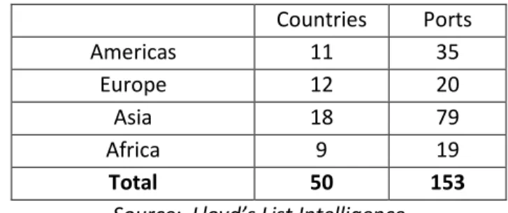
Table 1 Distribution of ports and countries in the sample according to the continents
Countries Ports Americas 11 35 Europe 12 20 Asia 18 79 Africa 9 19 Total 50 153
Source: Lloyd’s List Intelligence
7 As shown in Source: Lloyd’s List Intelligence
, most of the ports are located in Asia, followed by Central, Latin and North America, Europe, and Africa. The dataset contains information about 6,410 maritime routes. For each route, we have the following descriptive variables:
port of departure and port of arrival,
country, region and continent of departure and arrival,
In addition to these categorical variables, we have the following continuous and discrete variables for each maritime route:
Average size of container vessels measured in twenty-feet equivalent units (TEU) operating between a port of departure and a port of arrival;
Number of ships between a port of departure and a port of arrival;
Number of trips between a port of departure and a port of arrival;
Number of operators (liner shipping container carriers) operating between a port of departure and a port of arrival;
Number of ships per operator on a maritime route.
We have also included in our analysis the bilateral sea-distance between the main container ports in each country. It was computed by Bertoli et al. (2016). The database is developed at the country level and, if the two ports belong to the same country, the distance is set at zero. This variable shows the relative length of each maritime route.
Another variable at a country level which we use for the analysis is the Liner Shipping Bilateral Connectivity Index (LSBCI) which was developed by Hoffmann et al. (2014). LSBCI is an extension of UNCTAD’s country level Liner Shipping Connectivity Index (LSCI). The LSBCI includes the following components: 1) the number of transshipments required to get from country A to country B; 2) the number of direct connections common to both country A and country B; 3) the geometric mean of the number of direct connections of country A and of country B; 4) the level of competition on services that connect country A to country B; 5), the
8
size of the largest ships on the weakest route connecting country A to country B (Fugazza and Hoffmann, 2016).
Finally, the descriptive variable Trade Direction is a descriptive variable and allows us to analyze the imbalance of container trade between developed and less developed countries. We use the analytical classification made by the World Bank of the world's economies based on estimates of gross national income (GNI) per capita for 20146. Countries classified as High Income states
are considered as Developed (D), while the remaining countries are considered “Less developed” (DL). We obtain therefore four types of trade directions, D-D, LD-LD, D-LD and LD-D.
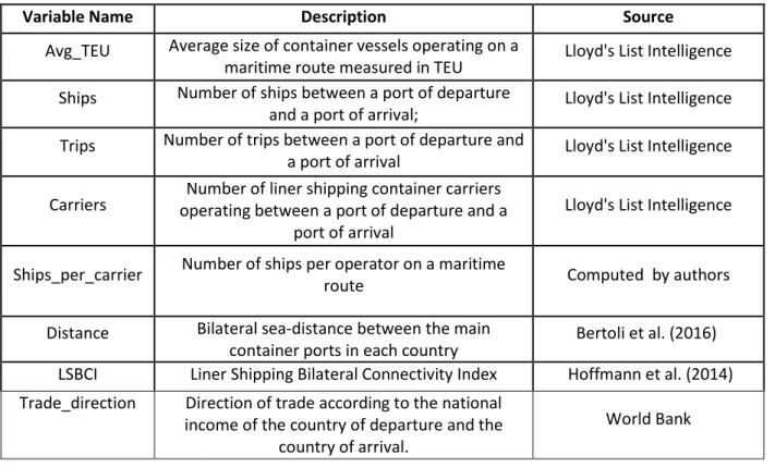
Table 2 Variables used in this study
Variable Name Description Source
Avg_TEU Average size of container vessels operating on a
maritime route measured in TEU Lloyd's List Intelligence Ships Number of ships between a port of departure
and a port of arrival; Lloyd's List Intelligence Trips Number of trips between a port of departure and
a port of arrival Lloyd's List Intelligence Carriers operating between a port of departure and a Number of liner shipping container carriers
port of arrival
Lloyd's List Intelligence
Ships_per_carrier Number of ships per operator on a maritime
route Computed by authors
Distance Bilateral sea-distance between the main
container ports in each country Bertoli et al. (2016) LSBCI Liner Shipping Bilateral Connectivity Index Hoffmann et al. (2014) Trade_direction Direction of trade according to the national
income of the country of departure and the country of arrival.
World Bank
Error! Reference source not found. provides a summary of the variables that we have used for the PCA and Cluster Analysis. It should be highlighted that we decided to restrict the analysis to the long distance routes (more than 5000 km) due to the heterogeneous nature of the observations, we have decided to conduct the Multivariate Analysis on the routes with regular services. Therefore, the routes with less than ten carriers, twenty ships were excluded.
9
3.2. Principle Component and Cluster Analyses
Principle Component Analysis (PCA) was introduced by Pearson (1901) and later developed by Hotelling (1933). It is one of the oldest multivariate techniques. PCA allows us to reduce the dimensionality of a data set in which there are a large number of interrelated variables, while retaining as much as possible of the variation present in the data set (Jolliffe, 1986). This methodology is applied to a data table where rows are individuals and columns are variables. The maritime routes between each pair of ports (port of departure and port of arrival) are considered as active individuals, i.e contributing to the estimated inertia of the cloud of individuals. The following continuous and discrete variables play the role of active elements in the analysis: Avg_TEU, Ships, Carriers, Trips, Distance, Carriers_ships and LSBCI, meaning that the inertia (or variance) of the cloud of variables is calculated on the mere basis of these active variables. Supplementary elements are also included but do not contribute directly to the factor analysis, being simply projected on the factorial maps built up by active elements: Route_Country, Route_Continents, Route_Regions and Trade_Direction play the role of illustrative discrete variables. The supplementary elements make it possible to illustrate the principal components.
We have also divided the maritime routes into different clusters by applying the Hierarchical Agglomerative Clustering Analysis based on prior Principle Components. The distance between the clusters has been computed by the Ward’s Method (Ward Jr, 1963).
4. Results
In this part are described the results. The first section provides descriptive statistics related to the whole dataset of 6,410 maritime routes. In the second and third sections are depicted the results of the PCA and cluster analyses for a subset of 800 maritime routes. Finally, the typology
10
of the maritime routes as well as the absolute concentration in terms of number of ships per carrier are presented.
4.1. Descriptive statistics
By looking first at the whole sample, we analyze the degree of competition on 6,410 maritime routes connecting 153 ports from 50 countries. Error! Reference source not found. provide descriptive statistics of the variables used in this study:
Table 3 Descriptive statistics for the whole dataset (6,410 routes)
Variable name Count Mean Std.
Deviation Minimum Maximum TEU 6,410 4,299.77 3,015.23 80.00 18,270.00 Ships 6,410 25.20 54.07 1.00 1,237.00 Carriers 6,410 11.14 17.90 1.00 264.00 Trips 6,410 99.70 277.10 1.00 5,510.00 Distance 6,410 6,771.12 5,906.48 0.00 22,374.60 Ships_per_carrier 6,410 1.86 1.21 1.00 19.00 LSBCI 5,630 0.55 0.15 0.19 0.86
As we can see in Error! Reference source not found., the dataset contains heterogeneous maritime routes. There are routes with only one ship operating between the port of origin and the port of arrival. The average size of ships, which is a proxy for economies of scale, also varies significantly: the mean is 4,299.77 and the maximum value is 18,270. On average, there are 25 ships and 99.7 trips per route. The average number of ships per carrier is 1.86, but some carriers can deploy up to 19 ships on a single route. Unfortunately, the distribution of market shares per route between operators, which would allow calculation for classical concentration indicator, was not available in this dataset. The high mean value of LSBCI (0.55) indicates that countries in the sample are relatively well connected between each other.
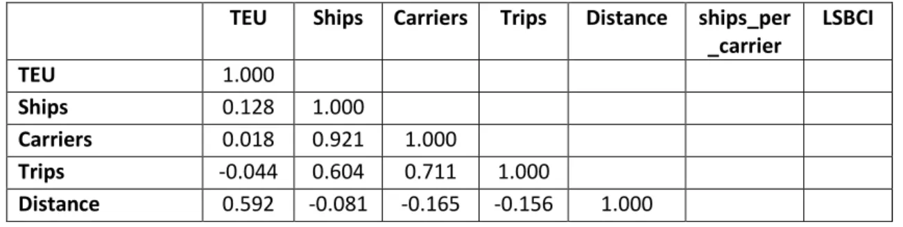
Table 4 Pearson's correlation matrix of the variables related to 6,410 routes TEU Ships Carriers Trips Distance ships_per
_carrier LSBCI TEU 1.000 Ships 0.128 1.000 Carriers 0.018 0.921 1.000 Trips -0.044 0.604 0.711 1.000 Distance 0.592 -0.081 -0.165 -0.156 1.000
11
Ships_per_carrier 0.407 0.328 0.205 0.165 0.191 1.000
LSBCI 0.283 0.278 0.242 0.213 0.042 0.227 1.000
There is an expected strong correlation between the number of carriers and that of ships. Also not surprising is the high positive correlation between the latter and the number of trips. However, the positive correlation coefficient between Distance and TEU indicates that the average size of operating ships increases with the distance between the port of origin and destination. Economies of scale would therefore increase with distance and may reduce the number of competing carriers. The number of ships per carrier, which is a proxy for the size of shipping companies, is also higher on the routes where these big vessels operate. Distance between ports would therefore be a key variable of lower competition through higher economies of scale acting as entry barriers.
Regarding the regional container trade, there are some fundamental differences across regions. In the dataset, the maritime routes are well distributed between “Developed” and “Less developed” countries. There are 1,766 routes between Developed countries (D-D), 1,414 routes connecting “Developed” and “Less developped” states (D-LD), 1,447 routes between Less developed and Developed nations (LD-D) and 1,783 routes link exclusively less developed states (LD-LD).
Table 5 Mean values according to the direction of the trade. D refers to “Developed” countries and LD refers to “Less Developed” ones. Developed states are those considered as "high income" countries by
the World Bank
Mean (D-D) Mean (D-LD) Mean (LD-D) Mean (LD-LD)
TEU 5,073.47 4,683.84 4,725.07 2,883.67 Ships 30.52 24.81 24.49 20.82 Carriers 12.86 10.97 10.86 9.81 Trips 145.59 91.71 93.17 65.87 Distance 7,298.05 7,921.28 7,575.73 4,684.00 Ships_per_carrier 2.21 1.80 1.84 1.51 LSBCI 0.61 0.55 0.55 0.48
Error! Reference source not found. reveals the relative imbalance according to the level of
income of the countries in the sample. The mean values of all variables are the highest on the maritime routes connecting “Developed” states (DD). It indicates that on these routes, the relative connectivity of the ports is also high and the traffic is the most intensive. The average
12
size of operators is also greater (2.21 ships per operator), which indicates more concentrated markets.
On the other hand, the containerized trade between ”Less developed” (Low income, Lower middle income, and Upper middle income countries) is less concentrated and the average values of all variables are the lowest ones. It is interesting to highlight that the maritime routes NS and SN are not perfectly symmetrical. The average size of ships on the “D-LD” routes are on average smaller and their number is slightly higher than those operating on the “LD-D” routes. This indicates a regional misbalance of the trade going from “Developed” to “Less developed” countries and vice versa. The services on the “LD-D” routes are more frequent and the vessels are smaller. In addition, there are more carriers on the “D-LD” routes. It could be explained by the fact that, often the vessels are not fully loaded on the ports in developed countries due to the low demand in less developed states. As a consequence, some carriers cooperate by forming alliances in order to optimize their costs.
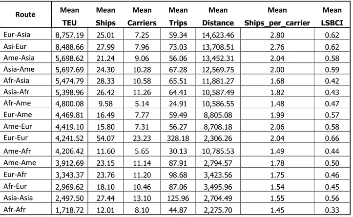
When we look at the trade between continents we observe that the container trade patterns differ considerably.
Route Mean Mean Mean Mean Mean Mean Mean
TEU Ships Carriers Trips Distance Ships_per_carrier LSBCI
Eur-Asia 8,757.19 25.01 7.25 59.34 14,623.46 2.80 0.62 Asi-Eur 8,488.66 27.99 7.96 73.03 13,708.51 2.76 0.62 Ame-Asia 5,698.62 21.24 9.06 56.06 13,452.31 2.04 0.58 Asia-Ame 5,697.69 24.30 10.28 67.28 12,569.75 2.00 0.59 Afr-Asia 5,474.79 28.33 10.58 65.51 11,881.27 1.68 0.42 Asia-Afr 5,398.96 26.42 11.26 64.41 10,587.49 1.82 0.43 Afr-Ame 4,800.08 9.58 5.14 24.91 10,586.55 1.48 0.47 Eur-Ame 4,469.81 16.49 7.77 59.49 8,805.08 1.99 0.57 Ame-Eur 4,419.10 15.80 7.31 56.27 8,708.18 2.06 0.58 Eur-Eur 4,241.52 54.07 23.23 328.18 2,306.26 2.04 0.66 Ame-Afr 4,206.42 11.60 5.65 30.13 10,785.53 1.49 0.44 Ame-Ame 3,912.69 23.15 11.14 87.91 2,794.57 1.78 0.50 Eur-Afr 3,343.37 23.76 11.20 98.68 3,423.56 1.75 0.46 Afr-Eur 2,969.62 18.10 10.46 87.06 3,495.96 1.54 0.45 Asia-Asia 2,497.50 27.44 13.10 125.96 2,704.49 1.55 0.56 Afr-Afr 1,718.72 12.01 8.10 44.87 2,275.70 1.45 0.33
13
shows that the biggest vessels operate between Europe and Asia. The average distance of these routes is also the highest. In addition, on average the vessels on Europe-Asia are with 269 TEUs bigger than those on Asia-Europe routes.
Table 6 Average values according to the continents of origin and destination
Route Mean Mean Mean Mean Mean Mean Mean
TEU Ships Carriers Trips Distance Ships_per_carrier LSBCI
Eur-Asia 8,757.19 25.01 7.25 59.34 14,623.46 2.80 0.62 Asi-Eur 8,488.66 27.99 7.96 73.03 13,708.51 2.76 0.62 Ame-Asia 5,698.62 21.24 9.06 56.06 13,452.31 2.04 0.58 Asia-Ame 5,697.69 24.30 10.28 67.28 12,569.75 2.00 0.59 Afr-Asia 5,474.79 28.33 10.58 65.51 11,881.27 1.68 0.42 Asia-Afr 5,398.96 26.42 11.26 64.41 10,587.49 1.82 0.43 Afr-Ame 4,800.08 9.58 5.14 24.91 10,586.55 1.48 0.47 Eur-Ame 4,469.81 16.49 7.77 59.49 8,805.08 1.99 0.57 Ame-Eur 4,419.10 15.80 7.31 56.27 8,708.18 2.06 0.58 Eur-Eur 4,241.52 54.07 23.23 328.18 2,306.26 2.04 0.66 Ame-Afr 4,206.42 11.60 5.65 30.13 10,785.53 1.49 0.44 Ame-Ame 3,912.69 23.15 11.14 87.91 2,794.57 1.78 0.50 Eur-Afr 3,343.37 23.76 11.20 98.68 3,423.56 1.75 0.46 Afr-Eur 2,969.62 18.10 10.46 87.06 3,495.96 1.54 0.45 Asia-Asia 2,497.50 27.44 13.10 125.96 2,704.49 1.55 0.56 Afr-Afr 1,718.72 12.01 8.10 44.87 2,275.70 1.45 0.33
A significant difference is observed between routes by number of trips. On Asia-Europe routes, the mean value of trips is 73 while on Europe-Asia ones it is 59 only, due the imbalance of trade between the two zones. A similar asymmetric pattern goes for the Asia-America route, with 67 trips and 24 ships on the front haul, against 56 trips and 21 ships on the back haul. However, the average size of companies measured in TEU per ship or in number of ships per company is very similar, unlike the Europe-Asia trade where, curiously, the average size of firms and vessels is slightly higher on the back haul (Europe to Asia) despite the imbalance. Almost symmetrical figures are reported on the routes between Europe and America. It indicates that the demand for container services are almost the same in the two continents. This trade balance facilitates carriers to operate efficiently, with an average firm size around 2 ships per carrier in both ways.
14
The intra-Asian and intra-African routes have different patterns. The average size of vessels as well as their absolute concentration measured by the number of ships per carrier is smaller than the intra-European and intra-American routes. The frequency of trips is fairly high on the intra-Asian trade routes compared to the intra-American trade, with 126 trips on average against 88, but both are far smaller than intra-European trade routes. Smaller vessels (1,719 TEU) operate on the intra-continental routes in Africa, where the bilateral connectivity between African countries is the lowest of the sample. Conversely, intra-Asian containerized trade is conducted between countries having a high connectivity. Appendix 1 depicts the maritime routes according to the region of origin and destination. Results show that the biggest vessels are deployed on the routes between East Asia, South-East Asia, Eastern Europe and Western Europe. On these routes, the average number of ships per vessels is the highest.
In summary, the overview of the 6,410 maritime show that there exist a significant misbalance between developed and less developed countries across regions. Maritime routes where larger companies compete (i.e. with a higher number of ships per carrier) are mainly associated with long distances and inter-regional trade between developed and less developed countries. Countries that are poorly connected tend to have a lower absolute concentration. In addition, intra-continental trade is more present between High Income countries and, as a consequence, their connectivity is also high. The market concentration (number of ships per carrier) is the highest on the routes connecting Developed (High income) countries and lowest on the links between “Less developed” ones. The trade routes “D-LD” and ”LD-D” are not symmetrical, which indicates a misbalance within the industry. When we look at the continent of origin and destination, it seems that the highest disparities are on the routes between Europe and Asia, and America and Asia. This regional imbalance explains the strategies of shipping companies to deploy bigger ships and to decrease the trips on the back haul routes from Europe and America to Asia.
15
Considering the heterogeneous nature of routes and the fact that competitors will focus their efforts on larger sub-markets, thus increasing competition, we have decided to restrict our analysis on the routes longer than 5,000 km. In order to include the routes with regular services, we have also removed from the sample those with less than 20 ships and 10 carriers. Finally, due to the presence of several outliers, routes with more than 1,000 trips were also removed. The final sample for the Principle Component Analysis consists of 800 maritime routes.
As active variables included in the PCA, we use Avg_TEU, Ships, Carriers, Trips, Distance, Ships_per_carrier and LSBCI. The supplementary variables are the following: Route_Country, Route_Continents, Route_Regions and Trade_Direction.
First we present the correlation coefficients of the active continuous and discrete variables.
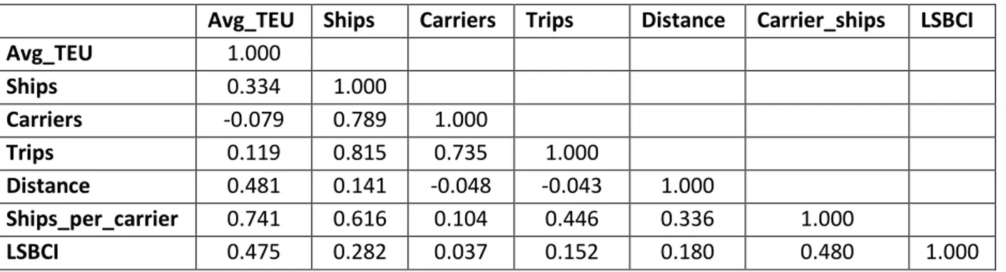
Table 7 Pearson's correlations matrix for the subset of 800 maritime routes
Avg_TEU Ships Carriers Trips Distance Carrier_ships LSBCI
Avg_TEU 1.000 Ships 0.334 1.000 Carriers -0.079 0.789 1.000 Trips 0.119 0.815 0.735 1.000 Distance 0.481 0.141 -0.048 -0.043 1.000 Ships_per_carrier 0.741 0.616 0.104 0.446 0.336 1.000 LSBCI 0.475 0.282 0.037 0.152 0.180 0.480 1.000
We observe similar Pearson coefficients as in the correlation matrix of the whole sample of 6,410 routes (see Error! Reference source not found.). However, the correlation between the variables ships and carriers is lower in this subset of data. In addition, the trips and ships seem to have a stronger positive relation. The correlation coefficient of Avg_TEU and Ships_per_carrier as well as Avg_TEU and Carriers_ships are higher than those related to the previous dataset. When we conduct the Principle Component Analysis, all variables are standardized.
16
First we study the inertia of the principle components by analyzing the presence of correlation between variables and the components.
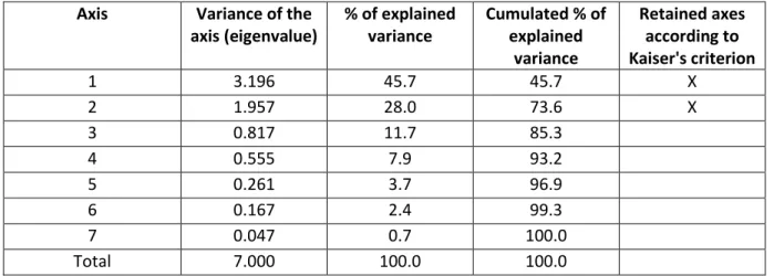
Table 8 Explained variance by component in the PCA analysis Axis Variance of the
axis (eigenvalue) % of explained variance Cumulated % of explained variance Retained axes according to Kaiser's criterion 1 3.196 45.7 45.7 X 2 1.957 28.0 73.6 X 3 0.817 11.7 85.3 4 0.555 7.9 93.2 5 0.261 3.7 96.9 6 0.167 2.4 99.3 7 0.047 0.7 100.0 Total 7.000 100.0 100.0
shows the Eigen value associated with each component, the percentage of explained variance and the cumulated percentage. Following the Kaiser’s criterion, we have decided to retain the first two components. Their cumulative percentage of explained variance is 73.6%.
Next we evaluate the contribution of variables to each of the two components. As shown in
Error! Reference source not found., the average size of containerships, the distance between
ports, ships per carrier and LSBCI have a significant and positive correlation with the first component and negative with the second one. On the other hand, the number of ships, carriers and trips correlate positively with both axes.
Table 9 Correlation coefficients of active variables with the axis and the contribution of the active variables to the axis
Correlations between active variables and factors
Contributions of the active variables to the axes (in %)
Axis 1 Axis 2 Axis 1 Axis 2
Avg_TEU 0.617 -0.665 11.9 22.6
Ships 0.910 0.336 25.9 5.8
Carriers 0.601 0.702 11.3 25.2
Trips 0.767 0.521 18.4 13.9
17
Ships_per_carrier 0.812 -0.386 20.6 7.6
LSBCI 0.518 -0.420 8.4 9.0
Active variables which have a major contribution in the construction of the first component are the number of ships and trips and, to a lesser extent, the average size of carriers. In other words, the most active routes are those where the traffic is intensive. Although linked to the first component, the weight of Distance is more limited compared to its influence on the second factor (negative correlation) where the number of carriers plays an opposite role (positive correlation). Therefore, the first component is related to the market size in terms of traffic and frequency of services, while the second component is associated with the increasing returns to scale of carriers facing long distance trade. Dropping the LSBCI variable and retaining the whole sample in the analysis -which is not presented here to avoid tedious presentation-, these two dimensions appear even more clearly: the first component captures the number of ships, trips and ships per operator, while the second axis introduces the negative correlation between the distance (associated with the average size of ships) and the number of carriers. Long distance hauls commands the absolute concentration of the market, with fewer and larger operating carriers.
18
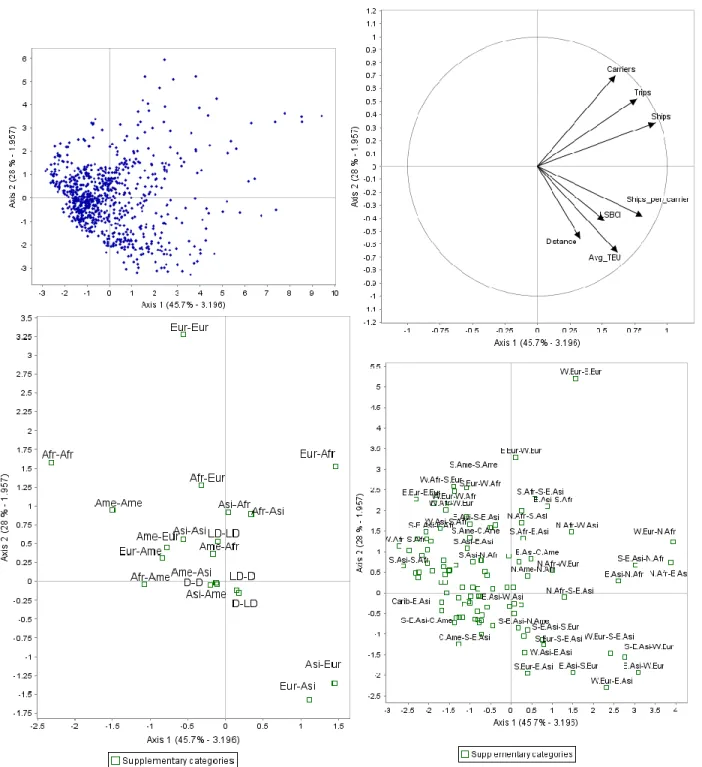
Figure 1: On the upper-left corner: the factorial map of individuals; On the upper- right corner: representation of the active continuous variables; On the lower-left corner: representation of the supplementary categorical variables related to the Trade Direction and the Trade between continents;
On the lower-right corner: representation of the supplementary categorical variables related to trade between regions.
Looking at the illustrative variables related to the containerized trade between continents, we can see that within-Europe trade substantially contributes to the second axis. This route is
19
situated on the upper-left corner of the graph, which means that smaller vessels and a higher number of carriers operate on the intra-European trade routes. Intra-African trade is opposed to the routes connecting Europe and Asia. At the regional level, we can clearly see that the outliers in the sample are the routes connecting Western Europe and Eastern Europe. In addition, on the second axis are opposed Eastern Europe-Western Europe and South Europe- Eastern Asia routes. The former has a shorter sea distance, smaller vessels and more carriers than the latter. On the first axis, we can distinguish several groups based on the regions of origin and arrival. The routes connecting South-East or East Asia and Northern Africa can be characterized have more ships, trips and ships per carrier. On the other hand, routes between South Asia and South Africa, Caribbean and Central America, Caribbean and East-Asia, and South East Asia and Central America are perhaps more peripheral with a lower carrying capacity. Therefore, maritime routes have different characteristics and it seems useful to define different clusters based on the PCA active variables and described by both active and supplementary variables.
4.3. Cluster Analysis
The purpose of the Cluster Analysis is to classify a set of objects. The hierarchical method consists of agglomerating individuals which have similar or close values on active variables. This “cluster” is treated as one individual in a new matrix. This process continues until the optimal number of clusters is found and retained. To visualize these clusters, we build a hierarchical tree called dendrogram (see Figure 2). This tree can be considered a sequence of nested partitions from the most precise (in which each individual is a class), to the most general one (in which there is only one class where all inertia is lost) (Husson et al., 2017). As in previous section, we have used the same sample (800 maritime routes) to conduct the clustering analysis.
20
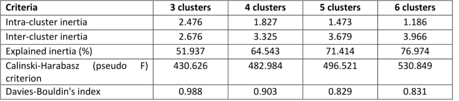
Table 10 Indicators of the quality of the identified clusters following Agglomerative Hierarchical Clustering
Criteria 3 clusters 4 clusters 5 clusters 6 clusters
Intra-cluster inertia 2.476 1.827 1.473 1.186 Inter-cluster inertia 2.676 3.325 3.679 3.966 Explained inertia (%) 51.937 64.543 71.414 76.974 Calinski-Harabasz (pseudo F) criterion 430.626 482.984 496.521 530.849 Davies-Bouldin's index 0.988 0.903 0.829 0.831
Error! Reference source not found. depicts that the optimal number of clusters is four. Even
though, the Calinski-Harabasz criterion and Davies-Bouldin's index suggest that the optimum number of clusters are six and five respectively six and five, it should be highlighted that the inertia loss by forming six clusters is very small, less than 10%. Therefore, we have decided to retain four clusters. The quality of the clusters is relatively good due to the low intra-cluster and the high inter-cluster inertia (or variance). The former refers to the deviation between each point and the center of gravity of the cluster to which it belongs, while the latter is computed based on the deviation between each center of gravity for a specific cluster and the overall center of gravity.
21
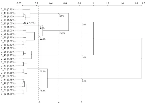
Figure 2 Dendrogram, Agglomerative Hierarchical Clustering based on the Ward criterion for the subset of 800 routes
Figure 2 shows the Hierarchical tree (Dendrogram) of the 800 maritime routes. By choosing to retain four clusters, we explain 64.5% of the total variability. These four clusters are depicted on the two axes that we have retained following the PCA (Figure 3). In the barycenter of cluster 1 is the maritime route connecting Tanjung Pelepas, Malaysia and Lagos, Nigeria. In 2014, between these two ports 36 ship with an average size of 4,293 TEU and 2.25 ships per carrier were operating. A typical representative of cluster two is the maritime connection between Tanjung Pelepas, Malaysia and Hamburg, Germany. There are 85 ships with a mean size of 9,850 TEU and 4.25 carriers per ships. Cluster three is represented by routes similar to the one between Shenzhen, China and Manzanillo, Mexico (89 ships, 6040 TEU and 2.07 ships per carrier). Finally, routes such as Ningbo-Zhoushan, China and Port Said, Egypt belong to the fourth cluster. On this route, there are 251 ships with an average size of 9,232 TEU and 4.45 ships per carrier.
22
Figure 3 Graphical representation of the four clusters on the first two PCA axes
Figure 3 provides a graphical representation of the four clusters. Some outliers and maritime routes close to the center of gravity of each cluster are shown as well. In order to have a better idea about the general characteristics of the four clusters, we provide the most significant statistics sorted out by a mean test for each one of them.
4.3.1. Cluster 1, transatlantic lines with low concentration (463 maritime routes)
The first cluster is the biggest one which includes 463 maritime routes. It is characterized by all seven active variables.
Table 12 Cluster 1, descriptive statistics of the supplementary variables and Error! Reference source
not found. shows that most of the routes in this cluster are between Developed (D) countries
23
transatlantic routes are over-represented in this first cluster. All mean variables are slightly lower than the mean values for the whole sample of 800 routes, the number of ships even representing nearly half the sample mean.
Table 11 Cluster 1 descriptive statistics of the active variables
Characteristic variables Category mean Overall mean Category Std. deviation Overall Std. deviation Test-value Probability Distance 10,548.800 11,354.700 3,781.090 4,172.200 -6.400 0.000 LSBCI 0.556 0.597 0.105 0.109 -12.463 0.000 Carriers 17.879 22.656 5.418 11.588 -13.659 0.000 Avg_TEU 5,381.440 6,529.610 1,602.970 2,552.900 -14.901 0.000 Trips 111.095 174.604 60.626 137.482 -15.305 0.000 Ships_per_carrier 2.109 2.619 0.442 0.994 -17.008 0.000 Ships 37.043 60.546 11.669 45.545 -17.097 0.000
Table 12 Cluster 1, descriptive statistics of the supplementary variables Variable label Characteristic
categories % of category in group % of category in set % of group in category Probability Trade_direction D-D 37.1 33.6 63.9 0.008 Trade_direction D-LD 21.8 25.6 49.3 0.003 Route_Continents Eur-Ame 14.7 10.4 81.9 0.000 Route_Continents Ame-Eur 11.0 7.9 81.0 0.000 Route-regions S.Eur-N.Ame 5.6 3.5 92.9 0.000 Route_Continents Ame-Ame 5.6 3.8 86.7 0.001
The absolute concentration within this cluster is relatively low, with 2.1 carriers per ship on average, a vessel size below average and only 18 carriers against 23 per route in the selected sample.
4.3.2. Cluster 2, low degree of competition (170 maritime routes)
Some 170 maritime routes are included in the second cluster. All active variables except the number of trips are significant. This group is mainly linked with the second component (Table 14 Cluster 2, descriptive statistics of the supplementary variables). The routes are significantly longer
24
(14,730 nautical miles) and characterized by fewer carriers operating nearly 4 ships on average and deploying rather large vessels (Avg_TEU is 10,149 TEU).
Table 13 Cluster 2, descriptive statistics of the active variables
Characteristic variables
Category mean
Overall mean Category Std. deviation Overall Std. deviation Probability Avg_TEU 10,148.800 6,529.610 1,468.070 2,552.900 0.000 Ships_per_carrier 3.764 2.619 0.946 0.994 0.000 LSBCI 0.687 0.597 0.058 0.109 0.000 Distance 14,729.900 11,354.700 3,821.480 4,172.200 0.000 Ships 69.624 60.546 26.788 45.545 0.002 Trips 170.953 174.604 80.117 137.482 0.348 Carriers 18.559 22.656 5.634 11.588 0.000
Table 14 Cluster 2, descriptive statistics of the supplementary variables
Variable label Characteristic categories % of category in group % of category in set % of group in category Probability Route_Continents Eur-Asi 41.2 11.1 78.7 0.000 Trade_direction D-L 35.3 25.6 29.3 0.001 Route_Continents Asi-Eur 34.1 11.0 65.9 0.000 Route-regions W.Eur-E.Asi 13.5 2.9 100.0 0.000 Route-regions S.Eur-E.Asi 11.8 2.5 100.0 0.000 Route-regions E.Asi-W.Eur 10.0 2.8 77.3 0.000 Route-regions S-E.Asi-W.Eur 8.2 2.0 87.5 0.000 Route_Continents Ame-Asi 6.5 14.8 9.3 0.000 Trade_direction L-L 6.5 16.3 8.5 0.000
From a regional perspective, this cluster gathers nearly all front and back hauls between Europe and Asia which represent three quarters of the cluster. The ports of departure or arrival for these lines have greater connectivity (nearly 10 points higher) than the rest of the sample. Absolute concentration of this sub-market is undoubtedly higher than previous cluster.
4.3.3. Cluster 3, high degree of competition (135 maritime routes)
There are 135 routes in the third cluster, mainly between Asia and America. The trade between China and USA is substantial in this group. Unlike the second cluster, this group is mainly linked
25
with the first component (market size). In this cluster, there are considerably more ships and trips than average. The variables which characterized the cluster are therefore Carriers, Trips and Ships. The average distance in this group is the shortest, with 9,549.44 km. On the other hand, competition on the routes is relatively intense between smaller carriers (2.46 ships per carrier, against 2.62 in the sample). The average size of vessels (around 5,300 TEU) is comparable to that of Cluster 1.
Table 15 Cluster 3, descriptive statistics of the active variables
Characteristic variables
Category mean
Overall mean Category Std. deviation Overall Std. deviation Probability Carriers 37.630 22.656 9.900 11.588 0.000 Trips 304.052 174.604 140.208 137.482 0.000 Ships 91.437 60.546 26.711 45.545 0.000 LSBCI 0.608 0.597 0.100 0.109 0.102 ships_per_carrier 2.464 2.619 0.513 0.994 0.023 Distance 9,549.440 11,354.700 3,245.700 4,172.200 0.000 Avg_TEU 5,336.050 6,529.610 1,530.720 2,552.900 0.000
Table 16 Cluster 3, descriptive statistics of the supplementary variables
Variable label Characteristic categories % of category in group % of category in set % of group in category Probability Route_Continents Asi-Ame 20.7 14.1 24.8 0.013 Route_Continents Ame-Asi 20.7 14.8 23.7 0.025 Route-regions N.Ame-E.Asi 15.6 8.5 30.9 0.002 Route_Country USA-CHN 11.1 3.8 50.0 0.000 Route_Country CHN-USA 6.7 3.3 34.6 0.020 Route-regions E.Asi-C.Ame 5.2 2.0 43.8 0.010
4.3.4. Cluster 4, low degree of competition (32 maritime routes)
The last one is the smallest cluster, with only 32 maritime routes. This cluster is mainly linked with the first axis, like previous cluster, and the most significant variables describing it are also the number of ships, trips, and carriers. In this cluster are found the trade lines operated either between developed or between less developed countries located mainly in Eastern Asia and Western Europe.
26
Table 17 Cluster 4, descriptive statistics of the active variables
Characteristic variables
Category mean
Overall mean Category Std. deviation Overall Std. deviation Probability Ships 222.063 60.546 67.258 45.545 0.000 Trips 566.781 174.604 139.269 137.482 0.000 Carriers 50.375 22.656 14.711 11.588 0.000 Ships_per_carrier 4.581 2.619 1.161 0.994 0.000 Avg_TEU 8950.870 6529.610 1972.240 2552.900 0.000 LSBCI 0.666 0.597 0.064 0.109 0.000 Distance 12,701.600 11354.700 4563.120 4172.200 0.031
Table 18 Cluster 4, descriptive statistics of the supplementary variables
Variable label Caracteristic categories % of category in group % of category in set % of group in category Probability Trade_direction LD-LD 37.5 16.3 9.2 0.003 Route_Continents Afr-Asi 25.0 5.8 17.4 0.000 Route-regions E.Asi-W.Eur 15.6 2.8 22.7 0.001 Route_Continents Asi-Afr 15.6 5.4 11.6 0.024 Trade_direction D-D 12.5 33.6 1.5 0.006
The degree of competition on the routes in the last cluster is the lowest: on average, there are 4.58 ships per carrier. Surprisingly, these are the busiest routes, the mean values of the number of ships and trips are considerably higher than average, 266% and 244% respectively. As shown in Figure 3, most of the routes are between hub ports such as Port Said in Egypt situated near the
Suez Canal, the Port of Singapore -the biggest port in ASEAN-, the port of Rotterdam -biggest port in Europe- as well as the port of Shanghai, -biggest port in the world. This is confirmed by the higher connectivity degree (0.67), close to that observed in the second cluster. These direct connections between hub-ports seem to limit the degree of competition since, they are dominated mainly by large companies operating large vessels.
27
In summary, the cluster analysis allows us to identify four categories of maritime routes based on the active variables. We observe that the lowest degree of competition (4.58 ships per carriers) is within a small clusters of 32 very busy routes connecting large hub-ports. The second cluster also is constituted of routes with fewer large carriers connecting mainly Western Europe with Eastern and South-Eastern Asia. The degree of competition is the highest among the routes between developed countries (intra-American and Intra-European routes). The container flows on these routes are relatively symetrical which do not require a high degree of cooperation between carriers to optimize their costs (slot capacity). The degree of competition is also relatively high on the routes connecting America and Asia where substantial part of the trade is conducted between China and USA.
An Interactive Decision Tree (IDT) based on the CART approach (Breiman et al. 1984) scrutinizes the typology by highlighting the most discriminating continuous variables of the absolute concentration of maritime routes measured by the average size of vessels (Fig. 4).
Figure 4. Interactive Decision Tree of the average size of vessels in TEU
28
Starting with an average size of 4,596 TEU per ship (st.-dev. 3,053 TEU), the first criterion to split up the sample is the distance of the route in nautical miles, below or above 9,806 nautical miles. Then comes the size of companies proxied by the number of ships per carrier. For shorter routes, the threshold is below or above 2.05 ships per carrier. For longer routes, this threshold is below or above 2.9. In other words, the companies owning less than 2.05 ships on routes shorter than 9,806 miles will operate the smallest containerships (2,839 TEU). By contrast, those carriers owning more than 2.9 ships on routes longer than 9,806 miles will operate large containerships of 8,968 TEU on average. The last discriminating criterion to increase further the average size of vessels is the connectivity of ports (LSBCI>0.53): operating vessels between hub ports is likely to increase the size nearly up to 10,000 TEU.
5. Conclusions
The degree of competition on the maritime routes was evaluated through the simplest concentration ratios available in the Lloyd’s List database, which are the number of ships per carrier and the average size of containerships deployed on the route. Unfortunately, unlike other studies focusing on a more limited number of routes, we did not have access to the distribution of market shares between liner companies for every route. Firstly, a descriptive statistics analysis of a sample of 6,410 routes between 153 ports reveals a regional misbalance between ports of origin and destination, particularly between Asia and Europe, and Asia and America. The biggest vessels are deployed on these routes because of the long distance and the high degree of port connectivity with other ports, especially between Europe and Asia. These routes are also the most concentrated. The highest levels of competition measured by these simple instruments is observed on the intra-African routes, which can be characterized as the shortest distance between ports, smallest vessels, the lowest number of trips and the worst bilateral country connectivity. Furthermore, when we look at the origin and destination across regions, we conclude that the highest level of absolute concentration of the market is between
29
Eastern Asia and Eastern Europe, South-East Asia and Eastern Europe, Southern Europe and Western Asia, and Western Europe and South-East Asia. It was found that competition is stiffer on the routes connecting mainly less developed regions such as Northern Africa and Eastern Asia.
Considering the heterogeneous nature of the whole sample we have decided to focus on the longer distance routes where are conducted many trips and multiple container vessels operate. Therefore, the sample size was limited to 800 routes. By applying Principle Component Analysis, we have identified two components which summarize the seven active variables and explain 73.6% of the variance. The first component rather relates to the market size, frequency of services and competition (number of ships, trips, carriers) while the second rather illustrates a certain form of absolute concentration (average size of ships) positively linked with the length of the route. For this limited sample, the two components are not so much independent one from the other, unlike the same analysis conducted over the whole sample of maritime routes where these two dimensions are less linked together.
The PCA-based cluster Analysis has allowed us to identify 4 distinct clusters. The first one includes mainly transatlantic routes. These are the routes where competition is less intense (lower number of ships, trips, carriers than average) which can be explained by low level of regional misbalance, which allows companies to operate efficiently and probably without having to share slot capacity with their competitors. The third cluster is similar to the first one and includes mainly routes between Asia and America. It is slightly more concentrated even though the distance and the average size of vessels are almost the same.
On the other hand, the second cluster is made up mainly with routes between Europe and Asia. The absolute market concentration is higher in this cluster, 3.76 ships per carrier. The distance and size of vessels have the highest mean values among the clusters. The group with the lowest degree of competition is in the fourth cluster, which has the largest hub ports in the network and despite the lower mean values of distance and the size of the ships than the second cluster, the level of market concentration is the highest. These results suggest that the distance, frequency of services and the size of the ships do have an impact on the degree of competition.
30
However, between major hub-routes were registered the highest frequency of services and at the same time the highest degree of monopolization. This is confirmed by the interactive regression tree explaining the average size of vessels: the criterion of distance comes first to explain this variable, followed by the size of the company and the connectivity index.
In Summary, we have shown that large distance routes between connected ports are in general more concentrated in absolute terms (fewer companies operating larger vessels), exploiting the large economies of scale on these routes. However, the degree of competition varies across regions of origin and destination. The competition looks more intense on intra-African and intra-Asian routes and also between less developed countries. The routes where the degree of competition is also relatively high is intra-continental trade in Europe and America. On the other hand, the trade misbalance between Asia and America and Asia and Europe might be one of the main reason for the relatively higher concentration on these routes. The PCA has shown that the Hub-and-Spoke network of the maritime transport leads to a smaller number of shipping companies operating a larger fleet of bigger vessels between the largest ports and these routes have the highest degree of concentration.
Additional studies should be conducted to analyze the nature of competition exclusively between the largest hub-ports in the maritime network or between smaller (feeder) ports. Additional data such as, the distribution of market shares per carrier on specific routes, the exact number of containers transported by each vessels from the port of origin to the destination as well as the amount of transshipments by vessel would allow researchers to understand better the nature of competition within the containerized trade network.
References
Agarwal, R. and Ergun, Ö. (2010): 'Network design and allocation mechanisms for carrier alliances in liner shipping. Operations research', 58, 1726-1742.
Anderson, C. M., Park, Y.-A., Chang, Y.-T., Yang, C.-H., Lee, T.-W. and Luo, M. (2008): 'A game-theoretic analysis of competition among container port hubs: the case of Busan and Shanghai. Maritime Policy & Management', 35, 5-26.
31
Asgari, N., Farahani, R. Z. and Goh, M. (2013): 'Network design approach for hub ports-shipping companies competition and cooperation. Transportation Research Part A: Policy and Practice', 48, 1-18. Bertoli, S., Goujon, M. and Santoni, O. (2016): 'The CERDI-seadistance database’.
Breiman, L., Friedman, J., Olshen, R. and Stone, C. (1984): 'Classification and Regression Trees, Wadsworth International Group, Belmont, California (1984). Google Scholar'.
Cariou, P. (2008): 'Liner shipping strategies: an overview. International Journal of Ocean Systems Management', 1, 2-13.
Cariou, P. and Wolff, F.-C. (2006): 'An analysis of bunker adjustment factors and freight rates in the Europe/Far East market (2000–2004). Maritime Economics & Logistics', 8, 187-201.
Clark, X., Dollar, D. and Micco, A. (2004): 'Port efficiency, maritime transport costs, and bilateral trade. Journal of development economics', 75, 417-450.
Dagnino, G. B. and Rocco, E. 2009. Introduction–coopetition strategy: A “path recognition” investigation approach. Coopetition Strategy. Routledge.
De Oliveira, G. F. and Cariou, P. (2015): 'The impact of competition on container port (in) efficiency. Transportation Research Part A: Policy and Practice', 78, 124-133.
Fraser, D. R., Notteboom, T. and Ducruet, C. (2016): 'Peripherality in the global container shipping network: the case of the Southern African container port system. GeoJournal', 81, 139-151.
Fugazza, M. and Hoffmann, J. (2016): 'Bilateral Liner Shipping Connectivity since 2006.”. Policy Issues in International Trade and Commodities, Study Series'.
Ha, Y. S. and Seo, J. S. (2017): 'An Analysis of the Competitiveness of Major Liner Shipping Companies. The Asian Journal of Shipping and Logistics', 33, 53-60.
Hirata, E. (2017): 'Contestability of Container Liner Shipping Market in Alliance Era. The Asian Journal of Shipping and Logistics', 33, 27-32.
Hoffmann, J., Van Hoogenhuizen, J. and Wilmsmeier, G. Developing an index for bilateral liner shipping connectivity. IAME 2014 Conference Proceedings. Presented at the International Association of Maritime Economists (IAME), Norfolk, United States, 2014.
Hotelling, H. (1933): 'Analysis of a complex of statistical variables into principal components. Journal of educational psychology', 24, 417.
Hurdle, G. J., Johnson, R. L., Joskow, A. S., Werden, G. J. and Williams, M. A. (1989): 'Concentration, potential entry, and performance in the airline industry. The Journal of Industrial Economics', 119-139. Husson, F., Lê, S. and Pagès, J. 2017. Exploratory multivariate analysis by example using R, Chapman and Hall/CRC.
Insight, G. and Boston, M. 2005. The application of competition rules to liner shipping, European Commission.
Jolliffe, I. T. 1986. Principal component analysis and factor analysis. Principal component analysis. Springer.
32
Liu, Q., Wilson, W. W. and Luo, M. (2016): 'The impact of Panama Canal expansion on the container-shipping market: a cooperative game theory approach. Maritime Policy & Management', 43, 209-221. Notteboom, T. and Yap, W. Y. (2012): 'Port competition and competitiveness. The Blackwell Companion to Maritime Economics', 549-570.
Notteboom, T. E. (2002): 'Consolidation and contestability in the European container handling industry. Maritime Policy & Management', 29, 257-269.
Panayides, P. M. and Wiedmer, R. (2011): 'Strategic alliances in container liner shipping. Research in Transportation Economics', 32, 25-38.
Pearson, K. (1901): 'LIII. On lines and planes of closest fit to systems of points in space. The London, Edinburgh, and Dublin Philosophical Magazine and Journal of Science', 2, 559-572.
Rau, P. and Spinler, S. (2016): 'Investment into container shipping capacity: A real options approach in oligopolistic competition. Transportation Research Part E: Logistics and Transportation Review', 93, 130-147.
Sanchez, R. J. and Wilmsmeier, G. 2011. Liner shipping networks and market concentration, Edward Elgar: Cheltenham.
Song, D.-W. (2002): 'Regional container port competition and co-operation: the case of Hong Kong and South China. Journal of Transport Geography', 10, 99-110.
Sys, C. (2009): 'Is the container liner shipping industry an oligopoly? Transport policy', 16, 259-270. Unctad 2017. Review of Maritime Transport 2017. Review of Maritime Transport. United Nations Conference on Trade and Development.
Wang, H., Meng, Q. and Zhang, X. (2014): 'Game-theoretical models for competition analysis in a new emerging liner container shipping market. Transportation Research Part B: Methodological', 70, 201-227.
Ward Jr, J. H. (1963): 'Hierarchical grouping to optimize an objective function. Journal of the American statistical association', 58, 236-244.
Yang, J., Wang, G. W. and Li, K. X. (2016): 'Port choice strategies for container carriers in China: a case study of the Bohai Bay Rim port cluster. International Journal of Shipping and Transport Logistics', 8, 129-152.
Yap, W. Y., Lam, J. S. and Notteboom, T. (2006): 'Developments in container port competition in East Asia. Transport Reviews', 26, 167-188.
Yeo, G.-T., Roe, M. and Dinwoodie, J. (2008): 'Evaluating the competitiveness of container ports in Korea and China. Transportation Research Part A: Policy and Practice', 42, 910-921.
33
Appendices
Appendix 1: Regional container trade between the 153 ports in the sample.
Mean TEU
Mean Ships
Mean
Carriers Mean Trips
Mean Distance Mean Ships_per _carrier Mean LSBCI E.Asi-E.Eur 15377 15.00 3.00 62.00 14363 5.00 0.533 E.Eur-E.Asi 13423 9.00 3.00 21.00 21543 3.00 0.537 S-E.Asi-E.Eur 12166 7.00 1.67 31.33 13645 3.00 0.503 E.Eur-S-E.Asi 10889 10.00 2.33 30.33 13520 3.56 0.468 W.Eur-E.Asi 10003 26.08 6.94 55.86 19624 2.66 0.676 E.Asi-W.Eur 9867 32.33 8.07 79.29 18183 2.90 0.682 W.Eur-S-E.Asi 9524 48.71 10.65 135.10 15161 3.91 0.627 E.Asi-S.Eur 9173 24.12 6.75 57.12 14289 2.67 0.630 S-E.Asi-W.Eur 9036 56.34 12.31 172.28 15311 3.62 0.639 S-E.Asi-S.Eur 8900 36.82 11.57 101.61 11573 2.79 0.611 E.Asi-N.Afr 8897 28.00 8.50 58.62 13440 1.69 0.484 N.Afr-E.Asi 8714 35.37 8.76 68.57 15427 1.73 0.456 W.Eur-W.Asi 8669 30.08 9.36 63.19 9259 3.03 0.591 S.Eur-E.Asi 8337 15.96 5.65 31.91 16184 2.31 0.633 S-E.Asi-N.Afr 8146 52.07 13.27 132.07 11374 2.12 0.444 S.Ame-S-E.Asi 7820 30.88 12.88 93.25 17892 1.71 0.473 E.Asi-W.Asi 7806 14.16 6.69 24.82 9889 1.77 0.574
34 S.Ame-S.Afr 7736 51.50 27.50 152.50 8195 1.87 0.450 N.Afr-S.Ame 7643 30.50 14.00 138.00 10240 2.17 0.477 S.Eur-W.Asi 7642 25.12 7.24 67.12 6097 3.94 0.577 S.Eur-S-E.Asi 7584 29.29 9.18 82.07 11561 2.61 0.572 W.Asi-E.Asi 7500 17.37 6.70 26.19 10676 1.89 0.604 S-E.Asi-S.Ame 7368 31.11 12.33 114.44 18065 1.93 0.466 W.Eur-S.Asi 7281 18.42 7.74 48.68 11910 2.19 0.553 S.Ame-S.Asi 7186 8.00 4.00 12.67 15385 1.90 0.399 C.Ame-W.Asi 7172 1.33 1.33 1.67 19255 1.00 0.418 S.Afr-S.Ame 7081 30.50 17.50 94.50 8195 1.74 0.450 S.Ame-N.Afr 6845 15.75 7.25 86.25 12140 1.86 0.447 S.Asi-W.Eur 6665 18.71 7.79 45.54 12018 2.19 0.553 S.Afr-W.Eur 6656 12.43 5.29 59.57 12830 3.04 0.519 E.Asi-S.Ame 6637 34.17 14.00 87.57 16245 2.37 0.484 W.Eur-S.Afr 6637 14.00 6.29 58.86 12831 2.78 0.519 W.Asi-W.Eur 6611 14.68 5.90 34.45 9218 2.49 0.586 S.Ame-E.Asi 6609 20.62 9.08 43.50 18768 1.90 0.486 W.Asi-Carib 6575 6.50 4.50 8.50 15880 1.69 0.339 Carib-W.Asi 6509 8.00 4.50 8.50 15880 3.19 0.339 S.Ame-W.Eur 6288 18.90 9.29 89.48 10796 1.90 0.479 N.Afr-S-E.Asi 6220 44.86 10.95 124.95 11206 1.84 0.406 W.Asi-C.Ame 6218 2.40 1.60 2.60 18124 1.50 0.415 S.Eur-S.Asi 6119 8.59 3.35 27.65 8521 2.14 0.525 N.Ame-S-E.Asi 6066 11.30 4.14 29.02 13613 2.25 0.529 W.Eur-S.Ame 5997 15.80 8.04 74.44 10837 1.74 0.478 S.Asi-S.Eur 5996 10.83 4.54 33.00 8570 2.18 0.520 Carib-S.Asi 5936 5.50 2.50 5.75 17715 3.36 0.371 S-E.Asi-N.Ame 5887 12.80 4.92 35.18 13726 2.11 0.555 N.Afr-W.Asi 5847 34.58 11.89 80.58 5904 1.75 0.416 S.Ame-W.Asi 5803 1.50 1.50 2.00 15706 1.00 0.398 E.Asi-N.Ame 5701 28.36 11.72 83.95 8903 2.11 0.682 Carib-E.Asi 5666 11.31 6.92 22.46 17531 1.63 0.451 N.Ame-E.Asi 5648 27.22 11.21 79.14 10025 2.05 0.683 W.Asi-N.Ame 5600 11.09 5.91 24.75 16982 1.77 0.543 N.Ame-S.Asi 5580 10.67 4.63 23.25 17515 2.22 0.536 W.Asi-S-E.Asi 5564 28.00 10.19 41.89 6854 2.03 0.514 E.Asi-Carib 5532 17.33 10.08 48.17 14885 1.65 0.459 S-E.Asi-W.Asi 5470 29.36 12.64 43.50 6675 1.85 0.507 N.Afr-N.Ame 5437 10.47 5.42 21.78 10009 1.51 0.524 N.Afr-S.Asi 5418 23.67 10.33 52.56 7793 1.59 0.439 N.Ame-W.Asi 5234 12.26 5.80 28.49 16795 2.14 0.547