SSD Technology Enables Dynamic Maintenance of Persistent High-Dimensional Indexes

HAL Id: hal-01305651

https://hal.inria.fr/hal-01305651

Submitted on 21 Apr 2016

HAL is a multi-disciplinary open access

archive for the deposit and dissemination of

sci-entific research documents, whether they are

pub-lished or not. The documents may come from

teaching and research institutions in France or

abroad, or from public or private research centers.

L’archive ouverte pluridisciplinaire HAL, est

destinée au dépôt et à la diffusion de documents

scientifiques de niveau recherche, publiés ou non,

émanant des établissements d’enseignement et de

recherche français ou étrangers, des laboratoires

publics ou privés.

SSD Technology Enables Dynamic Maintenance of

Persistent High-Dimensional Indexes

Björn Þór Jónsson, Laurent Amsaleg, Herwig Lejsek

To cite this version:

Björn Þór Jónsson, Laurent Amsaleg, Herwig Lejsek. SSD Technology Enables Dynamic Maintenance

of Persistent High-Dimensional Indexes. ACM International Conference on Multimedia Retrieval 2016,

Jun 2016, New York, United States. �10.1145/2911996.2912065�. �hal-01305651�

SSD Technology Enables Dynamic Maintenance

of Persistent High-Dimensional Indexes

Björn Þór Jónsson

[email protected]

Laurent Amsaleg

[email protected]

Herwig Lejsek

[email protected]

ABSTRACT

In today’s world of ever-increasing multimedia collections, dynamically and persistently maintaining high-dimensional indexes is imperative for industrial applications. Since HDD performance is the main bottleneck in index maintenance, we investigate the impact of SSD technology. We use the NV-tree to drive our analysis, as the only high-dimensional index in the literature which has seriously addressed up-dates. Our simulation model indicates that an index of 1.5 billion descriptors can be built dynamically on a high-end SSD in just over four hours of disk time, which is more than 500x faster than using a high-end HDD. Relatively small in-vestment in the new SSD technology can thus make dynamic and persistent high-dimensional indexes very feasible.

Keywords

High-dimensional index; Index maintenance; SSDs; NV-tree.

1.

INTRODUCTION

Multimedia collections are getting increasingly large. As a result, there has been significant interest in the scalability of k-NN search [6, 1, 4, 2, 5, 3, 8]. But nearly all of this work has ignored the effect of the growth of the collections, effec-tively ignoring the need to perform updates on the collection and the resulting index structure.

A prototypical multimedia retrieval system works as fol-lows: First, each media item is described using one or more high-dimensional features. For large-scale collections, the resulting feature collection is much too large to fit in main memory and must be made persistent on disk. Then the high-dimensional features are somehow compressed into a smaller representation, sometimes only a few bytes, and in-serted into an indexing structure for efficient searches. In some cases, the final representation of the features may de-pend on the index and thus vary based on, for example, the distribution in the high-dimensional space.

In an industry setting with specific response time require-ments, it is necessary to maintain a persistent index of the

DOI:http://dx.doi.org/10.1145/2911996.2912065

0.0 0.5 1.0 1.5

Random Reads Random Writes Sequential Reads Sequential Writes

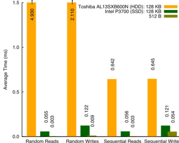
Average Time (ms) Toshiba AL13SXB600N (HDD): 128 KB 0.642 0.645 Intel P3700 (SSD): 128 KB 0.055 0.122 0.056 0.121 512 B 0.003 0.009 0.003 0.054 4.930 2.110

Figure 1: Performance comparison of a high-end

HDD (600 GB, $360) and a high-end SSD (400 GB,

$900). The y-axis (truncated) shows the time for

each of the operations on the x-axis, in milliseconds. The numbers show that SSDs are faster than HDDs by a factor of 5x to 1000x, depending on operation and data quantity. See Section 2.5 for more details.

entire collection. For example, it is not acceptable to keep a list of the newly added features, which is scanned sequen-tially in addition to searching the high-dimensional index, and then re-index the entire collection offline once in a while. First, the list of new features will grow steadily and with it the retrieval time, so performance will quickly become

un-acceptable. Second, full re-indexing will be a very

time-and resource-consuming process, which cannot be done fre-quently. Furthermore, in case of crashes, the persistent in-dex allows resuming the service immediately. The only way to achieve industry-standard service levels is to maintain a dynamic and persistent high-dimensional index!

1.1

Costs of Index Maintenance

In the short term, new features may be accommodated by inserting them into the appropriate index cell of the ex-isting structure. While standard logging techniques can be used to reduce cost, the changes must eventually be made persistent on disk. When the index fits in memory, a single write suffices; otherwise it may be necessary to read the cor-responding cell from disk and then write it back. Reading

and writing single cells results in random disk operations, which are costly using traditional hard-disk drives (HDDs). In the long term, inserting into existing cells leads to ex-cessively large cells which can negatively impact both re-trieval time and result quality. Index structure maintenance will therefore be required in order to split these cells and redistribute their contents. And again, those changes must be made persistent leading to disk reads and writes.

If the final representation of features depends on the index structure, further costs are incurred as the original features must be retrieved to compute a new representation against the modified index. Since the feature collection on disk is not aligned with the index, the original features of a single cell can be located anywhere in the feature collection and unlikely in close proximity to each other. Therefore, reading the features from disk can be a costly process of multiple random disk reads. This is particularly true with traditional HDDs which do not support small random reads well.

Recently, however, solid-state disks (SSDs) have appeared which have very different characteristics, as Figure 1 clearly demonstrates (see Section 2.5 for details of the figure). First, because they have no moving parts they are much faster

than HDDs (particularly high-end SSDs). Second, again

since they have no moving parts, the size of the IO im-pacts the performance much more than with HDDs, which in turn means that random reads become quite efficient, and in particular small random reads become very efficient. It is therefore of interest to observe the impact of SSDs on update performance of high-dimensional indexes.

1.2

Contributions

One of the most scalable high-dimensional indexing meth-ods in the literature is the NV-tree [4, 5]. It has been used for large-scale experiments and is currently the backbone of a professional copy-detection service indexing more than 150 thousand hours of video. It is also the only scalable high-dimensional index in the literature, as far as we know, where update performance has been seriously studied [4, 7]. We therefore use the NV-tree as the vehicle of our study.

In this paper we make the following contributions. We first review the NV-tree and identify the impact points of SSD technology on the performance of persistent and dy-namic index maintenance. We then present simulation re-sults which show that using a high-end SSD enables the insertion of 1.5 billion high-dimensional descriptors in just over four hours of disk time, which is more than 500x faster

than using HDD technology. Moreover, the results show

that for the NV-tree in particular, SSD technology allows a much simpler implementation of index maintenance than HDD technology, again due to its performance characteris-tics. We conclude that by using SSD technology, it is now very feasible to dynamically and persistently maintain high-dimensional indexes at a large scale.

2.

THE NV-TREE

Overall, an NV-tree is a tree index consisting of: a) a hierarchy of small inner nodes, which are kept in memory during query processing and guide the vector search to the appropriate leaf node; and b) larger leaf nodes, which are stored on disk and contain references to the actual features. In this section, we give describe the algorithms of the NV-tree for index construction, retrieval and maintenance. This description is brief and simplified; refer to [5] for details.

2.1

Index Creation

When the tree construction starts, all features from the collection are first projected onto a single projection line through the high-dimensional space. The projected values are then partitioned based on their position on the projec-tion line, thus partiprojec-tioning the root node of the tree. To build subsequent levels of the NV-tree, this process of pro-jecting and partitioning is repeated for each and every par-tition using a new projection line at each level, thus creat-ing the hierarchy of partitions that are represented by inner nodes. The process stops when the number of vectors in a partition falls below a limit designed to be disk I/O friendly. A new projection line is then used to order the vector iden-tifiers in each final partition and the ordered ideniden-tifiers are written to the leaf node on disk. Each feature is represented by a 4 byte identifier and, since the leaves are on average about 2/3 full, a total of 6 bytes are required per feature.

Two partitioning strategies co-exist inside the NV-tree. The first partitioning strategy is such that the distance be-tween partition boundaries at each level of the tree is equal. As the inner products between a set of high-dimensional vectors and a projection line typically form a normal distri-bution, the resulting partitions usually have very different cardinalities and dense areas are partitioned deeper than sparse areas. This first partitioning strategy is used at the upper levels of the NV-tree. The second partitioning strat-egy is used at the lowest levels of the tree: when a partition fits into a disk I/O, then data is partitioned according to an equal cardinality criterion (instead of an equal distance cri-terion). This switch to balanced partitioning occurs when a partition fit within 6 × 6 leaves, creating balanced leaf groups of up to 6 nodes containing up to 6 leaves each. The goal of this latter partitioning strategy is to enable efficient search in nearby leaves, as described below.

2.2

Nearest Neighbor Retrieval

The search first traverses the hierarchy of inner nodes of

the NV-tree. At each level of the tree, the query vector

is projected to the projection line associated with the cur-rent node. The search is then directed to the sub-partition with center-point closest to the projection of the query vec-tor. This process of projection and choosing the right sub-partition is repeated until the search reaches a leaf group.

At each level of the leaf-group, the two nearest branches are considered, or up to four leaves, and the nearest vectors along the projection lines are merged to form the final set of approximate nearest neighbors. As only two adjacent leaves are read at each level, at most four leaves will be read with this method. As these leaves are organized together on disk, they will span at most 12 pages, and can thus (with high likelihood) be read in a single disk read.

2.3

Index Maintenance

Insertion to NV-tree leaves proceeds as follows. When

the correct leaf node is found, using the exact same process as during search, the position within the leaf node is calcu-lated and the identifier is inserted in the designated position. During index creation, leaf nodes are not filled completely in order to leave space for such insertions. Once a leaf node is filled, however, it must be split in order to provide more storage capacity within the tree.

A basic method to split a node is very similar to the in-dex construction process. A new internal node is created

with two new leaf nodes as children. A projection line is then assigned to the internal node using the same method as during index construction. The contents of the full leaf node are projected along the projection line and inserted to the appropriate leaf. Each leaf is then also assigned a pro-jection line and the contents of the leaf ordered based on the projection to that line.

Using this basic method, however, the index would quickly become very deep, as each leaf would always be split into two leaves and all the new internal nodes would have only two children. A better method is to consider a group of l leaves together, and re-distribute their contents to l + ∆ leaves. The NV-tree goes one step further, and considers the leaf groups described above as the unit of splits; when that group exceeds 6 × 6 = 36 leaves, the group is split into 4 to 8 new leaf groups, depending on the distribution of the high-dimensional vectors in the original leaf group.

2.4

Re-Projection of Features

In order to project the contents of a filled leaf group, it is necessary to use the original features, as a) a new projec-tion line is (most likely) chosen for the internal nodes, and b) each new leaf also has a new projection line. Leaf nodes only contain feature identifiers, so the features themselves must be retrieved from disk. The features of the leaf group are randomly distributed over the whole feature collection, however, so their retrieval is a costly operation.

Three methods can be used to retrieve the features of a leaf group from the feature collection. First, it is possible to sequentially scan the entire collection. Second, it is possible to randomly read only the required features. Both are simple to implement, but neither is efficient using HDDs: the first methods reads too much data, while the second requires expensive random accesses.

A third method, proposed in [7], is to maintain an in-dependent feature database for each NV-tree—called par-tition files—which is organized in the same manner as the leaf groups. With this last method, only a small number of sequential disk reads are required to retrieve the features of the leaf group. When using HDDs, this method has been shown to be the most efficient [7], even though the redun-dant partition files must also be maintained during splits.

2.5

Expected Impact of SSDs

As mentioned above, Figure 1 compares two high-end disks from each category: HDD and SSD. Prices are ob-tained from allhdd.com and amazon.com, respectively. The performance of the SSD is obtained with actual performance measurements using the fio benchmark. The performance of the HDD, on the other hand, is extrapolated from [9] as follows: the average sequential throughput is used directly to calculate the cost of sequential operations and read/write access times is used as the cost of random operations. Based on Figure 1, we make the following observations:

• For the HDD, sequential operations are ∼10x faster

than random operations. Random writes are faster

than random reads due to buffering, as the disk buffers writes temporarily to improve performance. Small op-erations (not shown) take roughly the same time as larger operations.

• The SSD, in contrast, shows no difference between ran-dom and sequential operations. Reads are twice as fast as writes, due to properties of the storage medium.

• For the SSD, small operations are ∼10x faster than large operations, due to the absence of movable parts. • Overall, the SSD is 5–10x faster than the HDD for sequential operations and 10–100x faster for random operations.

• For small disk reads, however, the SSD is ∼1000x faster than the HDD. This is particularly beneficial for the re-projection of features during splits.

Overall, the expected impact of using SSDs on NV-tree maintenance is two-fold. First, due to the overall perfor-mance improvement, we expect the index maintenance to be significantly faster, making it feasible to dynamically main-tain persistent indexes. Second, due to the capacity for very fast small random reads, we expect that reading the features to re-project randomly from the large collection will be more efficient than maintaining the redundant feature database.

3.

PERFORMANCE EVALUATION

In this section, we study the performance of NV-tree main-tenance with both HDD and SSD technology. We first de-scribe our simulation model, which is similar to the one in [7], and then present the results.

3.1

Modeling NV-tree Maintenance

Assume that the feature collection consists of NF features

in SF blocks of 128 KB. We assume each feature is 132 bytes

(128 dimensions) and that the NV-tree requires 6 bytes per

feature. The NV-tree consists of NL leaves organized into

NG leaf groups. Each leaf is at most 4 KB, so each leaf

group is at most 36 × 4 = 144 KB. We assume that each leaf-group is stored in a contiguous chunk of space on disk and can be read or written with a single IO operation.

If partition files are maintained, there are also NG

par-tition files. The size of the parpar-tition file depends on the number of features it stores but overall, partition files are about 20 times larger than leaves. Since they also can be organized in a contiguous manner, reading or writing a par-tition file requires a number of sequential operations.

At insertion time, a system buffer is maintained which is organized the same way as the NV-tree. This system buffer contains feature identifiers and projected values, and in the case of partition files, also the feature itself. If the buffer fills up, it is flushed by sequentially reading all partitions and writing out with the added feature identifiers. For each partition file represented in the buffers, the end of the par-tition file is read, appended to and written again.

When a leaf is split, one random read is first performed to read the leaf group. The cost of a random read of a leaf

group is termed CRRL and given in Figure 1; we assume that

each such read is 128 KB. Then a random write of the leaf

group is required to persist the change (CRWL ). When the

entire leaf group is full and is split into four leaf groups, the writing phase consists of four leaf-group sized random writes

(4CRWL ). Note that when a partition is split, its features are

removed from the buffers. If partition files are maintained, similar operations must be performed; since partition files are about 20 times larger, however, the costs are higher.

The cost of re-projection of features during split of a leaf group G depends on the method used. As described in the previous section, there are three alternatives which we ex-plore: The first alternative is that of sequentially scanning

then entire collection of features; this costs SF× CL

0.1 1 10 100 1000 10000 100000 1e+06 1e+07 1e+08 0 250 500 750 1000 1250 1500

Total Elapsed Time (hours)

Inserted Features (millions) HDD: Scan Feature Collection

Read Partition Files Read Individual Features SSD: Scan Feature Collection Read Partition Files Read Individual Features

Figure 2: A comparison of total elapsed disk time for index maintenance using the high-end HDD (solid lines) and high-end SSD (dashed lines).

second alternative is to retrieve all the features from the

fea-ture collection; this costs SGCF

RR, where CRRF is the cost of

a small random read and SGis the number of features in the

leaf group. Finally, if partition files are maintained, they can

be read, which costs between CL

SRand 20CSRL , depending on

the size of the given partition file.

Initially, the NV-tree consists of 50 million descriptors. A total of 1.5 billion descriptors are then inserted, one by one, keeping track of the total elapsed time, as measured by the estimated IO time.

3.2

Simulation Results

Figure 2 shows the total elapsed time for both the HDD and the SSD from Figure 1. Let us focus first on the HDD (solid lines). As expected, the figure shows that scanning the collection (red) is the slowest method, while maintaining the partition files (yellow) is faster than reading individual features (green). Note that even though the reduced cost of reading partition files during leaf splits is partially offset by the cost of maintaining them during leaf-group splits, the maintenance cost is much smaller than the time savings. In total, however, inserting the 1.5 billion descriptors requires more than 2,000 hours of disk time, which is infeasible.

Turning to the SSD performance in Figure 2 (dashed lines) we first observe that the maintenance time is significantly re-duced compared to the HDD. In fact, for both full collection scan (red) and partition file scan (yellow), which are domi-nated by large sequential reads, the SSD is more than 10x faster, as sequential reads are ∼10x faster with the SSD. Reading the individual features (green), however, which is dominated by small random reads, is more than 1000x faster. Again, this is as expected, as the SSD is ∼1000x faster for

such reads. The most efficient method using the SSD—

reading individual features—takes just over 4 hours, which is more than 500x faster than using partition files on the HDD. Four hours of disk time for 1.5 billion descriptors is very feasible, even in demanding industry settings.

4.

CONCLUSIONS

We have argued that the performance of high-dimensional index maintenance is a very worthy subject of investigation in today’s world of large-scale and ever-increasing multime-dia collections: in order to offer industry-strength solutions with reliable retrieval performance, it is necessary to main-tain a dynamic and persistent copy of the high-dimensional index on disk. Since HDD performance is the bottleneck in such index maintenance, we have investigated the impact of SSD technology on the implementation of index mainte-nance. We have used the NV-tree to drive our analysis, as it is the only high-dimensional index in the literature which has seriously addressed updates.

Our results show that using SSD technology 1.5 billion can be inserted into the index in a matter of just over four hours. Furthermore, while a redundant copy of the entire feature collection was needed when using HDDs, a straightforward method of reading the required features randomly is by far the best solution using SSDs. These results mean that a very modest investment in the new SSD technology can simplify index maintenance and allow the dynamic and persistent maintenance of even large-scale high-dimensional indexes.

5.

ACKNOWLEDGMENTS

The authors wish to cordially thank Philippe Bonnet, Ivan Luiz Picoli, Max Enroth and Carla Villegas Pasco of the IT University of Copenhagen for their performance measure-ments of the Intel P3700 SSD card and related discussions.

6.

REFERENCES

[1] M. Douze, H. J´egou, H. Sandhawalia, L. Amsaleg, and

C. Schmid. Evaluation of GIST descriptors for web-scale image search. In Proc. CIVR, Santorini, Greece, 2009.

[2] H. J´egou, M. Douze, and C. Schmid. Product

quantization for nearest neighbor search. TPAMI, 33(1), 2011.

[3] H. J´egou, F. Perronnin, M. Douze, J. S´anchez,

P. P´erez, and C. Schmid. Aggregating local image

descriptors into compact codes. TPAMI, 34(9), 2012.

[4] H. Lejsek, F. H. ´Asmundsson, B. T. J´onsson, and

L. Amsaleg. NV-Tree: An efficient disk-based index for approximate search in very large high-dimensional collections. TPAMI, 31(5), 2009.

[5] H. Lejsek, B. T. J´onsson, and L. Amsaleg. NV-Tree:

nearest neighbors at the billion scale. In Proc. ICMR, Trento, Italy, 2011.

[6] T. Liu, C. Rosenberg, and H. Rowley. Clustering billions of images with large scale nearest neighbor search. In Proc. IEEE WACV, Austin, TX, USA, 2007.

[7] A. ´Olafsson, B. T. J´onsson, L. Amsaleg, and H. Lejsek.

Dynamic behavior of balanced NV-trees. Multimedia Systems, 17(2), 2011.

[8] X. Sun, C. Wang, C. Xu, and L. Zhang. Indexing billions of images for sketch-based retrieval. In Proc. ACM MM, Barcelona, Spain, 2013.

[9] Tom’s Hardware. All enterprise HDD charts.

http://www.tomshardware.com/charts/enterprise-hdd-charts/benchmarks,156.html, accessed Feb 3, 2016.