Decision support tool for the tanker second-hand market using data mining techniques

(1)

Decision Support Tool for the Tanker Second-hand Market Using Data Mining Techniques

by

Athanasios A. Karaindros

M.S. Mathematics University of Rhode Island 1998

B.S. Mathematics Brandeis University 1997

SUBMITTED TO THE DEPARTMENT OF OCEAN ENGINEERING IN PARTIAL FULFILLMENT OF THE REQUIREMENTS FOR THE DEGREE OF

MASTER OF SCIENCE IN OCEAN SYSTEMS MANAGEMENT AT THE

MASSACHUSETTS INSTITUTE OF TECHNOLOGY SEPTEMBER 2005

and to distribute publicly paper and electronic copies of this thesis document in whole or in part.

Signature of Author:

Department of Ocean Engineering August 31, 2005 Certified by: Accepted by: MASSACHUSETTS INSTiTUTE OF TECHNOLOGY

NOV

0 7 2005

IBIRARIES

Henry S. Marcus Professor of Marine Systems Thesis Supervisor

Lallit Anand Professor of Mechanical Engineering Chairman, Committee for Graduate Students

BAR"e

I .--- ________________________

(2)

(3)

by

Athanasios A. Karaindros

Submitted to the Department of Mechanical and Ocean Engineering On August 31, 2005 in Partial Fulfillment of the

Requirements for the Degree of Master of Science in Ocean Systems Management

ABSTRACT

This thesis proposes an innovative decision support tool intended for market leaders and those anticipating market states of "sale and purchase". This is feasible with the use of powerful data mining techniques and the construction of explanatory forecasting models. Data mining techniques seek and extract patterns from databases. These patterns can be used to reveal possible interactions between database variables and to predict values for future "sale and purchase" market states as an aid to decision-making. Possible users of such a tool are ship brokers, ship owners, shipyards and general brokers and investors. It is crucial to mention the rising need for decisional tools especially when asset play in shipping seems to increase its proportion among other investment practices.

Thesis Supervisor: Henry S. Marcus Title: Professor of Ocean Systems

(4)

ACKNOWLEDGEMENTS

Throughout the time I have spent in researching, structuring and writing my thesis, a couple of people have taken an interest in my work. I would like to take this opportunity to acknowledge the assistance of these people.

Dr. Henry S. Marcus, acting as my supervisor for the project. I have been able to make great use of his valuable knowledge and ideas. My supervisor was always willing to advise and assist me.

Dr. Nicholas M. Patrikalakis for his help, belief and encouragement throughout the difficult times.

Individuals, who prefer to remain anonymous, from: the Drewry Shipping Consultants, the Lloyds' Group, the Clarksons Research Group, Allied Shipbrokers and AK Shipping & Trading.

Mr. Sydney Levine of Shipping Intelligence.

All the staff in the Department of Ocean Engineering for their support and help.

Finally, I would like to thank my family and friends for their continued understanding, support and encouragement throughout all these years.

(5)

CONTENTS

1 IN TR O D U C TIO N ... 10

1.1 G ENERALITIES ... 10

1.2 CHARACTERISTICS OF TANKER SECOND-HAND MARKET ... 12

1.3 PROBLEM D EFINITION - REPORT STRUCTURE... 13

2 M ETH O D O LO G Y ... 15

2.1 D ATA COLLECTION ... 15

2.2 D ATA PREPROCESSING... 18

2.3 D ATA A NALYSIS AND M ODEL D EVELOPMENT ... 25

3 IMPLEMENTATION RESULTS ... 27

3.1 ZERO M ONTH M ODEL...27

3. 1.1 Form of the Zero M onth M odel... 27

3.1.2 Evaluation of the Zero M onth M odel ... 29

3.2 SIx M ONTHS M ODEL ... 35

3.2.1 Form of the Six M onths M odel... 35

3.2.2 Evaluation of the Six M onths M odel ... 37

4 DECISION SUPPORT TOOL -A CASE STUDY ... 43

4.1 D ECISION SUPPORT TOOL D EFINITION ... 43

4.2 CASE STUDY ... 44

5 C O N CLU SIO N S... 47

5.1 SUGGESTIONS FOR FURTHER RESEARCH ... 48

A PPEND IX A : N A M ES FILES ... 50

1 ZER O M O N TH M O D EL ... 51

2 SIX M O N TH S M O DEL ... 52

A PPEN D IX B : RESU LT FILES...53

1 ZER O M O N TH M O D EL ... 54

2 SIX M O N TH S M O D EL ... 62

APPENDIX C: STATISTICAL ANALYSIS RESULTS...70

1 D ESC R IPTIVE STA TISTICS... 71

2 CO R RELA TIO NS...72

REFEREN CES ... 74

(6)

LIST OF TABLES

Table 1: Descriptive Statistics for Vessels Characteristics ... 18

Table 2: Descriptive Statistics for Tanker 5 Years Old Average Price in $/DWT ... 21

T able 3: C orrelations ... 23

Table 4: C orrelations ... 29

T able 5: C orrelations ... 36

Table 6: Case Study Results ... 46

(7)

LIST OF FIGURES

Figure 1: The Age Profile of the Tanker Vessels ... 19

Figure 2: The Tonnage Profile of the Tanker Vessels ... 19

Figure 3: The Tonnage Profile of the Tanker Vessels ... 20

Figure 6: The Zero Month Model Fit on the first 20Training Cases of Tanker Vessels.... 30

Figure 7: The Zero Month Model Fit on the next Training Cases of Tanker Vessels...30

Figure 8: The Zero Month Model Fit on the next Training Cases of Tanker Vessels...31

Figure 9: The Scatter Plot for Zero Month Model Fit on Training Cases of Tanker Vessels ... 32

Figure 10: The Zero Month Model Fit on 20 First Testing Cases of Tanker Vessels...33

Figure 11: The Zero Month Model Fit on 20 NextTesting Cases of Tanker Vessels...33

Figure 12: The Zero Month Model Fit on 20 NextTesting Cases of Tanker Vessels...34

Figure 13: The Scatter Plot for Zero Month Model Fit on Testing Cases of Tanker Vessels ... ... .34

Figure 14: The Six Month Model Fit on 20 First Training Cases of Tanker Vessels...37

Figure 15: The Six Month Model Fit on 20 Next Training Cases of Tanker Vessels ... 38

Figure 16: The Six Month Model Fit on 20 Next Training Cases of Tanker Vessels ... 38

Figure 17: The Scatter Plot for Sic Month Model Fit on Training Cases of Tanker Vessels ... 39

Figure 18: The Six Month Model Fit on 20 First Testing Cases of Tanker Vessels ... 40

Figure 19: The Six Month Model Fit on 20 Next Testing Cases of Tanker Vessels...40

Figure 20: The Six Month Model Fit on 20 Next Testing Cases of Tanker Vessels...41 Figure 21: The Scatter Plot for Six Months Model Fit on Testing Cases of Tanker Vessels

.. .. .. .. .. .. .. .. .. .. .. .. .. .. .. .. . .. .. .. .... .. .. .. .. .. .. .. .. .. .. ... .. .. .. .. .. .. .. .. .. .. .. .. . 41.4

(8)

Synopsis

What is the main issue in the tanker second-hand market? To sell or purchase at the right price, at the right time. To accomplish both goals seems rather difficult especially in the chaotic and volatile system of the world shipping market. The common practice is to use expertise and information in order to follow market trends and stay at the safe side of revolution.

This thesis proposes an innovative decision support tool intended for market leaders and those anticipating market states of "sale and purchase". This is feasible with the use of powerful data mining techniques and the construction of explanatory forecasting models. Data mining techniques seek and extract patterns from databases. These patterns can be used to reveal possible interactions between database variables and to predict values for future "sale and purchase" market states as an aid to decision-making. Possible users of such a tool are ship brokers, ship owners, shipyards and general brokers and investors. It is crucial to mention the rising need for decisional tools especially when asset play in shipping seems to increase its proportion among other investment practices.

The report will be structured as follows: the first chapter will introduce past research papers in this cognitive field. It is essential to show research innovation and to mention the relative references, and the sources of the data and information. The tanker market will be described with an emphasis on "sale and purchase". It is crucial to reveal all possible interactions between tanker vessel prices and market state variables such as time charter rates, steel prices etc. Using expert judgment, an initial explanatory model will be constructed in order to build the final database and a function approximation model.

Data pre-processing will take place at the second chapter. By using descriptive statistics

methods, we'll try to define the following: * final database

* independent and dependent variables * form of the explanatory forecast model, * forecast time span and step,

* training, testing and cross validation dataset

Relations among the various parameters as well as between their current and past values or their moving averages are sought out through the calculation of the Pearson correlation coefficient. The main scope is to transfer the biggest proportion of necessary information from the data through the model to the dependent variable and at the same time avoid multi-colinearity and congestion problems.

The second chapter will describe and show the application of the methodology (data mining technique). The appropriate variables are then chosen and rule based, piecewise linear, multivariate models are developed in the form of trees using recursive partitioning of the training data set. The explanatory model will be fitted on training data and evaluated with data, out of training sample, using performance criteria. It is crucial to prove goodness of forecast and the ability to generalize. This is a critical issue and it is up to the modeller's ability to avoid overtraining and achieve generalization.

In the third chapter the results will be presented among with various criteria in order to evaluate model accuracy. After the training and testing process, it is common practice to present the results.

(9)

A Decision Support Tool (DST) will be presented in the fourth chapter and applied into predetermined cases. It is very significant to describe the utility and ascendancy of the proposed DST. Various criteria will be assessed in order to evaluate DST.

The conclusions of the report will be presented in the fifth chapter along with suggestions of future research directions.

(10)

1

INTRODUCTION

1.1 Generalities

The transportation of bulk liquids by sea generally requires the use of the tankers. The main types of tankers are for the transport of oil products, crude oil, chemicals, wine, molten sulphur or liquid gas.

Oil tankers form by far the largest fleet of specialist bulk vessels. The tanker fleet can be usefully subdivided into six segments: Handymax (10-50,000 dwt), Panamax

(50-70,000 dwt), Aframax (70-100,000 dwt), Suezmax (100-200,000 dwt), VLCC (200-300,000 dwt) and ULCC ((200-300,000 dwt). Each of these segments operates as a separate market, and from a ship design viewpoint, each has its own specific requirements. Tankers under 50,000 dwt are mainly operated for the transport of oil products and larger vessels for the transport of crude oil.

There are two different designs for oil tankers, single hull and double hull. Until 1990 almost all crude oil tankers had a single skin, using the hull as the main containment vessel and in 1996, 86% of the tanker fleet was single hull. IMO Regulation 13F required tankers ordered after July 6, 1993 to be of double hull construction as a protective measure against oil loss. The regulation laid down precise rules regarding the width of the double side and double bottom, but the principle was simple enough. There must be a second skin to limit the outflow of oil in the event of collision damage to the outer hull.

Cargo handling is an important aspect of tanker design. Rapid loading and discharge requires powerful pumps. Crude oil tankers rely on shore based facilities for loading, but carry their own cargo pumps for discharge. The pump room is generally located between the cargo tanks and the engine room. A network of pipes run along the deck, linking the cargo tanks to two banks of manifolds, one on each side of the ship. To load or discharge cargo, the manifolds are connected to the shore based pipe system by flexible hoses, which are handled by the ship's cranes. The flow of oil is controlled by valves operated from a control panel on the bridge and must conform to a plan which minimizes stress on the hull. Note that an incorrect load or discharge sequence can literally sink the vessel. Having introduced the market for tanker vessels, we are going to concentrate more on the pricing of tanker vessels rather than their special characteristics and design.

Vessel prices and their movements over time are of great importance to shipowners taking decisions regarding the purchase and sale of vessels. As Stopford (1997) notes, 'Typically, second-hand prices will respond sharply to changes in market conditions, and it is not uncommon for prices paid to double, or halve, within a period of a few months.' Furthermore, investors in the shipping industry rely not only on the profits generated from shipping operations, but also on capital gains from buying and selling

(11)

merchant vessels. In fact, some investors consider the latter activity more important than the former one since correct timing of sale and purchase can be highly rewarding compared to operating the vessel.

Shipping is a very volatile and risky market, while shipping cycles and speculative investments, in the newbuilding and S&P markets, compound the industry's volatility. A shipowner's goal in the shipping industry is to improve overall performance, that is to maximize profits (or minimize costs) at an acceptable level of risk. This goal can be achieved by developing and implementing effective investment and chartering strategies. Successful strategies require selecting the right mix of assets. A combination of owned tonnage, long term contracts (time chartered tonnage or contracts of affreightment), short term coverage (spot market, consecutive voyages), as well as positions in the paper (derivatives) markets constitute the mix of assets that the shipping market agent has to decide upon in designing a successful strategy.

As market volatility increases, flexibility to react becomes more important. The design and implementation of a robust strategy for investment management and risk control is a highly complicated task in a cyclical and volatile market, like bulk shipping. It requires detailed and continuous market and risk analysis to detect market trends early on, and to incorporate them in the appropriate strategy decisions. The key factors of any strategy in the shipping industry are: (a) Timing of making an investment; (b) Asset mix that is the split between short and long term contracts, as well as the distribution of assets across market segments; and (c) Management of the inherent volatility of shipping markets, and the uncertainty around market forecasts.

It is argued that because vessels are the main asset which ship-owners hold in order to provide their freight service to the market, and since the sums involved in holding these

assets are the largest item in the ship-owner's cash-flow, changes in their values can make all the difference in terms of ending up with a profit or loss from their investments in the shipping sector. Often the contribution of asset play to the balance sheet is greater than operation of the vessel itself. The timing of the investment decisions is extremely important. Investors which have exercised successfully the "buy low - sell high" principle in the vessel's markets have ended up with hefty bank balances at the end of the day. A large number of ship-owners/companies rely on these (vessel) transactions to make a profit in the sector. Others make a loss, and fall substantially out of business, as the sums involved are large. For example, investors are only able to exploit correct anticipations of market upturns in the vessel value market. Thus, they would buy a vessel at a certain time period and wait until vessel prices increased to sell the vessel at a higher price. If prices fell they would make a loss.

The future development of second-hand tanker prices is investigated based on the assessment of their relationships to tanker freight rates and scrap values. The development of prediction models for future values of second hand prices based on freight rates and scrap values is the product of the project's investigation and the main intention of this study.

(12)

In detail, the thesis is divided into five chapters:

" The introduction that describes second hand market and defines the problem; * The methodology chapter where pre-processing takes place along with the data

mining technique, definition and implementation. The explanatory models are developed, trained, and tested;

* The results chapter where methodology output is presented and evaluated with various criteria.

* The Decision support tool and the case study chapter. In this chapter, the tool is described and presented through a case study.

The present document is an innovative research attempt to model the second-hand market and provide a useful tool to every party involved in tanker vessel brokerage. The innovation of this thesis, is that it is a first attempt at analyzing and predicting the second-hand tanker market using explanatory models and specifically data mining techniques.

1.2 Modelling Ship Prices and Characteristics of the Second-hand Tanker Market

The objective of the thesis is to analyze the second-hand tanker market and produce a decision support system. In order to achieve this, a sedulous market study is necessary. It aims to reveal all crucial interactions between the second-hand tanker prices and the shipping and global economic system.

The formulation mechanism for the second-hand tanker prices is not clearly known but depends on the global socioeconomic status and the shipping industry. Moreover, prices are the output of the equilibrium of supply and demand levels for sea transport tanker services, new building and steel prices. Second-hand tanker prices are formed under numerous excitations and the corresponding qualitative and quantitative impact in price formulation would be very difficult to be revealed.

Vessel prices fluctuate as wildly as freight rates. This is expected, as vessel prices of the expected cash-flows from operating the vessel over its lifetime plus the present value of the expected scrap value of the vessel at the end of its life. The largest contributor to the fluctuations in vessel values are expected freight rates. Expected discount rates (used to calculate the present values) and expected operating costs are relatively constant (with the exception of bunker prices). Strandenes (1984) investigates the price formation in the dry bulk and tanker sectors. She finds that prices are influenced more by changes in the long-term profits rather than changes in current operating profits. She also argues that such a relationship could be viewed as support for the validity of the rational expectations assumption in ship price formation. Beenstock and Vergottis (1989) show that second-hand vessel prices are positively related to expected discounted profits, to discounted newbuilding prices and to a wealth over the stock of the fleet variable; the latter two factors reflecting the state of the market for vessels as well as the wealth/income effect of investors.

(13)

Traditional approaches for modeling ship prices are mainly based on general and partial equilibrium models using structural relationships between a number of variables such as orderbook, newbuilding deliveries, scrapping rate, freight rates, bunker prices etc. (see Beenstock and Vergottis, 1989 and Tsolakis et al., 2003, among others). More recent studies have applied real options analysis for determining ship prices; this valuation framework takes explicitly into account the operational flexibility in ship management, in terms of choosing between spot and period time-charter contracts and switching between lay-up and trading modes (see Dixit and Pindyck, 1994, Tvedt, 1997 and Bendal and Stent, 2004, among others). Kavussanos (1996, 1997), by using GARCH type models, shows that the second moments (the variances) of vessel prices are time-varying and are affected by factors such as time-charter rates, interest rates and oil prices. Moreover, these variances, reflecting vessel price risks, are time-varying.

Another strand of research has examined whether markets for ships are efficient and whether prices are formed rationally. For example, Kavussanos and Alizadeh (2002), Hale and Vanags (1992) and Glen (1997), among others, test the validity of the Efficient Market Hypothesis (EMH) in the formation of second-hand dry bulk prices. These studies argue that the failure of the EMH may be attributed to either the existence of time-varying risk premia, or may reflect the existence of arbitrage opportunities in the market.

1.3 Problem Definition - Report Structure

All parties in vessel brokerage processes are using expert judgement to solve most of the aforementioned issues. The major problem, in my opinion, is to estimate the vessel price in an accurate, fast, and easy way. Moreover, this estimation has to be correlated with the current market status and trends. This means that experts should be continuously informed of current issues in shipping, freight rates and price values, in order to imprint this knowledge to a useful decision support tool.

This thesis aims to overcome these difficulties and develop a tool able to: * Produce present second-hand vessel price estimations

* Produce future second-hand vessel price estimations * Ensure high level of accuracy

* Adapt new second-hand market trends and innovations * Adjust functionality according to user needs

The decision support tool will be the main product of this thesis. A database will be formed and used to explore market characteristics. Various statistical methods will be implemented in order to come up with solid results regarding the second-hand tanker market as well as the interactions with other markets and variables. A data mining technique will be applied in order to form explanatory models. Two models will be developed. The first one aims at producing estimations for present second-hand tanker values while the second one aims at producing future tanker values in six months. The model's dependent variable will be the second-hand tanker prices. The independent variables will consist of two main clusters. The first cluster includes vessel attributes

(14)

and the second shipping market and global economic variables. Numerous criteria will be used in order to evaluate the models and their goodness of fit. The overall output will be a decision support tool which will be demonstrated with a case study.

It should be noted that the proposed model, like many models, is not able to predict dramatic changes in market direction because it is based on historical data.

(15)

2 METHODOLOGY

In the context of this thesis, it was decided to use Data Mining Techniques in order to reveal relationships and patterns among data. Generally, Data Mining Techniques are used as a powerful operational research tool that enables researchers to form and seek rules of dependency among variables in a database. Data mining techniques have many areas of implementation. A similar research attempt was the one undertaken by Lyridis et al (2004b) where data mining models have been used to analyze and predict tanker new building prices and order book size. The method parcels out all of the possible multidimensional solution spaces seeking for clusters where a linear multi-parameter model can describe the relationship between the target variable (second-hand vessel price) and the informational variables.

This approach supports the initial statement that an explanatory model is more suitable to predict future and estimate present prices than a univariate model such as ARIMA or GARCH -Lyridis et al (2004a, b). The main advantage of an explanatory model is that by the use of an explanatory vector of informational variables, information is transferred to the target variable except for the information that is included in the precedent values of the target variable. Two specialized explanatory models will be constructed and used as "function approximation modules" for current and future values of tanker vessels second-hand prices.

The second-hand tanker vessel prices are examined in relation to their tonnage capacity, scrap values and tanker market freight rates, not only in their current levels but also in their past ones with a lag time of up to twelve months. The second-hand tanker prices are expressed in million $. Conclusions from this approach will contribute to the development of predictive models.

2.1 Data Collection

Availability of data is basically the most crucial parameter when trying to solve a problem. The shipping sector, data and general information is valuable and difficult to collect and hence very expensive. Given that this is an academic attempt and there was no funding for purchase of the necessary information, the writer had to fill the database by transferring data from hard copy journals and magazines or by contacting large shipping companies and colleagues with access or subscriptions to data providers. Therefore, it is necessary to make a note on how difficult it is to find and collect data. Sometimes data from different sources differ substantially, other times categories in which data is organized (by various sources) are not steady in time. These problems are faced on a case by case basis, by reorganizing data in larger categories, by evaluating the reliability of each source etc.

In this case, data for the tanker second-hand prices, Aframax timecharter rates and Aframax scrap values were drawn from the Clarksons Research Studies the Drewry Shipping Statistics and Economics, the Lloyds' Shipping Economist, Mr. Sydney Levine of Shipping Intelligence, as well as from my advisor Henry S. Marcus.

(16)

Monthly values of the tanker second hand prices were collected from November 1986 to July 2005 mainly from the Clarksons Research Studies. These were then processed and filtered based on ship size in order to include vessels with tonnage from 60,000 to 100,000 dwt.

Freight rates in $ per day for tankers were also collected from Clarksons Research Studies, the Drewry Shipping Statistics and the Lloyd's Shipping Economist on a monthly basis from November 1986 to July 2005 for the following time charter contract: Vessel type: Aframax

Tonnage: 95,000 dwt Age: early 90's

Hull: single

Duration: one year.

According to Clarksons, the one year tanker rates, expressed in $/day, are collected on a weekly basis for average ships of the type specified above. It should be mentioned that this is an average index, and therefore Clarksons have included earlier charter contracts starting from 1986 with vessels built prior to 1986. This is actually explained in the Clarksons website under publications. The collection is done in the same way for spot market rates, by requesting brokers to fill in a weekly pro-forma with the latest rate for each ship type or by estimating the likely rate acceptable to an owner in the absence of any fixtures.

An important variable that describes the tanker second-hand market is the scrap values variable. Scrap values in million $ were collected from the Lloyd's Shipping Economist on a monthly basis from November 1986 to July 2005.

It is important to explain the importance of each of the variable embedded in the database. Expert judgment is a common practice prior to pre-processing in order to form the appropriate explanatory model which contains most of the information without congestion and multi-colinearity effects. It is obvious that precedent prices will affect future ones. Market feeling is well described in precedent price values along with variables describing "second-hand market state". A variable that describes the Aframax and Panamax second-hand market and leads market progression is believed to be the freight rates variable. It is also important to note that by using a moving average of such a variable, one can obtain more than just a single value for the market state, which is a volatile variable.

The scrap values variable is the connection between the shipping market and the global industry state. For example, steel prices have reached historical highs due to China's enormous economic boom. This has pushed new building and scrap prices to extremely high levels. The second-hand market, which is located between the shipping and the global industry markets, has also shown an increase due to these virtual frontiers. Therefore, the inclusion of these variables was necessary for the formulation of the explanatory model.

The pre-processing procedure is what determines the exact form of the two explanatory models.

(17)

The available data has the following variables:

date variable denoting exact time of vessel transaction nominal variable denoting the name of the vessel ordinal variable denoting the year of vessel built continuous variable denoting the vessel tonnage ordinal variable denoting the vessel age

continuous variable denoting Time Charter Rate continuous variable denoting Time Charter Rate before continuous variable denoting Time Charter Rate before continuous variable denoting Time Charter Rate before TR(-4) continuous varia TR(-5) continuous varia TR(-6) continuous varia TR(-7) continuous varia TR(-8) continuous varia TR(-9) continuous varia TR(-10) continuous varia TR(- 11) continuous varia TR(-12) continuous varia MATR(6) continuous varic Rate

MATR(6_12) co

average of Time Charter Rate

(6_12) of Scrap Value continuous continuous ble ble ble ble ble ble ble ble ble denoting Time denoting Time denoting Time denoting Time denoting Time denoting Time denoting Time denoting Time denoting Time Charter Rate Charter Rate Charter Rate Charter Rate Charter Rate Charter Rate Charter Rate Charter Rate Charter Rate before before before before before before before before before

1

2 3 month months months 4 months 5 months 6 months 7 months 8 months 9 months 10 months 11 months 12 months

able denoting 6 months moving average of Time Charter ntinuous variable denoting 12 to 6 prior months moving variable variable variable variable variable variable variable variable variable variable variable variable variable variable

denoting Scrap Value denoting Scrap Value denoting Scrap Value denoting Scrap Value denoting Scrap Value denoting Scrap Value denoting Scrap Value denoting Scrap Value denoting Scrap Value denoting Scrap Value denoting Scrap Value denoting Scrap Value denoting Scrap Value

before 1 month before 2 months before 3 months before 4 months before 5 months before 6 months before 7 months before 8 months before 9 months before 10 months before 11 months before 12 months

denoting 6 months moving average of Scrap Value continuous variable denoting 12 to 6 prior months moving variable denoting Vessel Price

variable denoting Vessel Price after six months

Page 17 of 78 date Name Year Built DWT Age TR TR(-1) TR(-2) TR(-3) continuous continuous continuous continuous continuous continuous continuous continuous continuous continuous continuous continuous continuous continuous SV 0 SV -1 SV -2

SV -3

SV -4

SV -5

SV -6

SV -7

SV -8

SV -9

SV -10

SV -11

SV -12 MASV MASV average PriceG Price6

(6)

(18)

2.2 Data Preprocessing

In forecasting values for the tanker second-hand prices, prediction periods of zero and six months were selected. It was decided to develop two forecasting models dedicated to different time spans:

1. Zero time lead: This forecast model is very useful in order to have an accurate estimation of the price of a Panamax or an Afamax tanker vessel relative to the current state of the shipping market.

2. Six months time lead: In general, it can be understood that an increased predictive period provides more time in which ship-owners can make decisions based on future estimates, but it also leads to less reliable prediction values. A period of six months is considered sufficient for decision making, especially when the current value is provided for comparison, while it leads to the development of more reliable models.

Models are based on the previous values of the dependent variables, which are the second-hand tanker prices, and freight rates, as well as the previous values of the independent variables, which are in each case, the Aframax scrap values up to a year ago. It is expected that when the shipping market is in a continuous good state, prices will continue to increase and vice versa. Another consideration for the development of the models is that the historical data for a single hull 95,000 DWT Aframax vessel time charter freight rates for the six and twelve month moving averages, may better represent the continuous state of the shipping market versus a single monthly value.

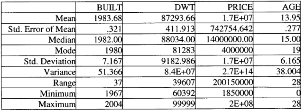
The descriptive statistics of the vessels included in the database are shown in the table below:

BUILT DWT PRIC AGE

Mean 1983.68 87293.66 1.7E+07 13.95

Std. Error of Mean .321 411.913 742754.642 .277 Median 1982.0C 88034.00 14000000.00 15.00

Mode 198C 81283 4000000 19

Std. Deviation 7.167 9182.986 1.7E+07 6.165

Variance 51.366 8.4E+07 2.7E+14 38.004

Range 37 39607 200150000 28

Minimum 1967 60392 1850000 0

Maximum 2004 99999 2E+08 2

Table 1: Descriptive Statistics for Vessels Characteristics

The age profile of the vessels under examination is presented in figure 1. The age mean value of the second-hand vessels participating in the sale-purchase process is 14 years.

(19)

AGE

100' 80-60m 40- d 0.0 5.0 10.0 15.0 20.0 25.0 2.5 7.5 12.5 17.5 22.5 27.5 AGE

Figure 1: The Age Profile of the Tanker Vessels

The tonnage profile in DWT of the vessels under examination is presented in figure 2. The mean value of the second-hand vessels' DWT is 87,293.7

DWT

100 ' 80' 60' 40-20. Std. Dev = 9182.99 Mean = 87293.7 ... N = 497.00 *0 qO q O 00 -0 0 *0 ?0 q% 00 DWT

Figure 2: The Tonnage Profile of the Tanker Vessels

Page 19 of 78 Q) C U_ 20 0 Std. Dev = 6.16 Mean = 14.0 N = 497.00 0 C C-a) LL

(20)

Decision Support Tool for the Tanker Second-hand Market Using Data Mining Techniques

The values in $ of the vessels under examination are presented in the histogram below. The mean value of the second-hand vessel prices is $17.7 million.

PRICE

200, 100

L

Z

0 Std. Dev = 16558598 MWan = 17714195.2 ________________ ___ N = 497.00 00 0 00 0 0 0 00 000 00 0 0 00 09,00, 0, 0 9,, ,00

*0 *0 *0 0o *o0 *?o *o0 *0 %

PRICE

Figure 3: The Tonnage Profile of the Tanker Vessels

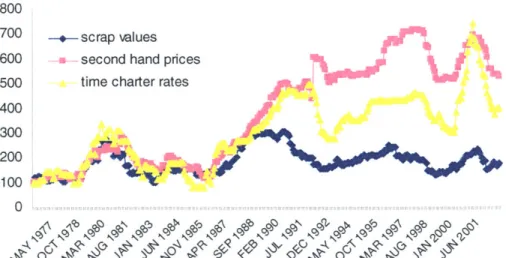
Figure 4, shows the variance of the: scrap values, second hand prices and the time-charter rates transformed. One can see the common variance and the high correlation. The figure also shows a short time lag between time charter rates and the other two attributes.

800

700 -+--scrap values

600 -- second hand prices

500 time charter rates

400/

200

0

Fse

Figure 4: Scrap Value, Second Hand Prices and Time-Charter Rates diagram

(21)

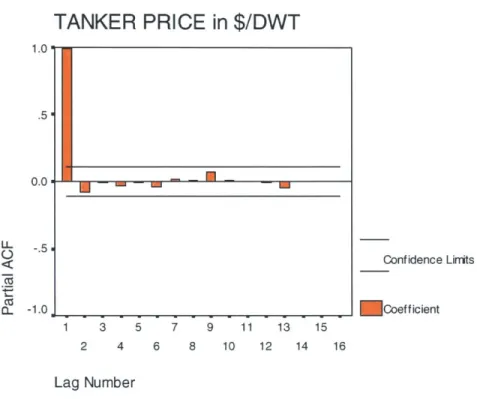
The next figure shows the partial autocorrelation function for the 5 year old average tanker prices in $ per DWT.

According to the partial autocorrelation chart, the second hand prices have one step dependence. The correlation factor at time lag 2 or higher is statistically insignificant and below the confidence limits.

TANKER PRICE in $/DWT

1.0 .5 0.0

U

1 - - - - 1 1 1-1 3 5 7 9 11 13 15 Confidence Limits Coefficient 2 4 6 8 10 12 14 16 Lag Number

Figure 5: Partial Autocorrelation Function for Second Hand Prices

The descriptive statistics of second-hand prices are shown in the table below:

Mean Std. Error of Mean Median Mode Std. Deviation Variance Skewness Std. Error of Skewness Kurtosis Std. Error of Kurtosis Range Minimum Maximum 262.9438 7.56501 297.8100 363.20 137.84108 19000.16249 .025 .134 -1.551 .267 419.36 66.30 485.66

Table 2: Descriptive Statistics for Tanker 5 Years Old Average Price in $/DWT

Page 21 of 78 CL -.5

-1.0

(22)

-Decision Support Tool for the Tanker Second-hand Market Using Data Mining Techniques

The following section discusses the criteria for the selection of the proper variables. The main criteria that were used in selecting the appropriate variables are the following:

1. The correlation between independent and dependent variables measured by the correlation factor. It is necessary to mention that the autocorrelation factor of the dependent variable was calculated in order to determine its use as an input variable. Finally all the cross-correlation factors were calculated, thereby introducing the phenomenon of time delay often observed in the tanker market. 2. The low multi-colinearity between the independent variables. Multi-colinearity

disorients the artificial neural networks and leads to poor performance by providing a piece of information multiple times. Multi-colinearity can be measured either by calculating the coefficient factors between each independent variable or by calculating the Variance Inflation Factor.

3. Supposing the existence of a set of k variables, the Variance Inflation Factor is

VIF = 1

calculated by the equation I - R2 where R is the coefficient of determination between an independent variable and the k-1 residual variables. As the variance inflation factor increases, so does the variance of the regression coefficient, making it an unstable estimate. Large VIF values are an indicator of multi-collinearity.

4. Expert judgment is an asset when dealing with the shipping market as well as thorough knowledge and analysis of the events that have influenced the second-hand tanker market during the past two decades.

Co-linearity (or multi-colinearity) is an undesirable situation where the correlations among the independent variables are strong. The relationship between the dependent and independent variables as well as just between the independent variables is assessed by calculating Pearson's correlation coefficient [Edwards (1984), Kutner et al (2003), Draper and Smith (1982)]. The only variables chosen for the development of the prediction models, are ones with high correlation to the dependent variables and low correlation between themselves. Those that show low correlation to the dependent variables are immediately omitted from the training data. Pearson's correlation factor is given by the following equation:

(N -1) 2X Y

tN

2 0 n

x (1)

where:

p ,pt ,t=l,2,...,N are two given time series

PX pY _{are the mean values of the X and Y time series respectively}

(23)

Y are the standard deviations of the X and Y time series respectively N is the number of data in each of the time series

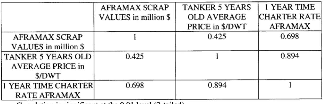
The correlations among variables of the database are shown in the table below:

AFRAMAX SCRAP TANKER 5 YEARS 1 YEAR TIME VALUES in million $ OLD AVERAGE CHARTER RATE

PRICE in $/DWT AFRAMAX

AFRAMAX SCRAP 1 0.425 0.698

VALUES in million $

TANKER 5 YEARS OLD 0.425 1 0.894

AVERAGE PRICE in $/DWT

1 YEAR TIME CHARTER 0.698 0.894 1

RATE AFRAMAX

Correlation is significant at the 0.01 level (2-tailed).

Table 3: Correlations

The bivariate correlations procedure computes Pearson's correlation coefficient with its significance levels. Correlations measure how variables or rank orders are related. Pearson's correlation coefficient is a measure of linear association. Pearson's correlation coefficient is between -1 and 1. When the coefficient is close to 1 it means that this two variables are perfectly positively correlated. For example, when the first variable increases the second will also experience an increase. When the coefficient is close to -1, if the first variable increases the second will experience a decrease. If the coefficient is close to 0 or between the critical values of ±1.96/4n, where n is the number of time series cases, the variables are considered to be uncorrelated.

It is obvious that the average price of the second hand tankers is strongly positively correlated with the time charter rates and the scrap values. Therefore, these two variables can be included in the explanatory model. That leads to the conclusion that an increase in tanker freight rates or scrap values impels an increase in the second-hand values and vise versa.

It is generally accepted that scrap values are dependent on the global iron prices. Iron prices affect both the scrap and new-building value markets. Since the second-hand price market lies between the new-building and the global iron price markets, the second-hand market is forced to react, in a similar manner, to the move of those other two markets. The scrap value variable is not included in the model not because I chose to disregard it but because the model itself ignored the scrap value variable. This is shown in the name files in the Appendix. One can see that the variables initially considered but not chosen by the model have the statement "ignore" next to them. It is crucial to check for multi-colinearity between database variables. An empirical rule is that variables with a bivariate correlation factor of more than 0.8 should not both be included in the model as independent variables. The correlation factor between time

(24)

charter rates and scrap values is 0.425, which is less than 0.8, and therefore both can be included as independent variables.

The development of models is done using a special software tool for developing rule-based predictive models from data. The tool is called Cubist and is an excellent data mining tool. The user determines the input data set, the test set, the target variables and the informational variables. All the above sets are located in individual files with formats specialized for cubist (Appendix A). The first essential file is the names file (e.g. now.names) which defines the attributes used to describe each case. The second essential file, the applications data file (e.g. now.data), provides information on the training cases that Cubist will use to construct a model. The entry for each case consists of one or more lines that give the values for all explicitly-defined attributes. Values are separated by commas and the entry for each case is optionally terminated by a period. The third kind of file used by Cubist is a test file of new cases (e.g. now.test) on which the model can be evaluated. This file has exactly the same format as the data file. In this application the cases have been split equally 50-50 into data and test files containing 200 and 200 cases respectively.

Generally, in order for both the training and the test dataset to be representative of all the possible (or as many as possible) market states in the shipping economy (from 1986-present), one must mix the data in a random manner and then split that into two sets. The train set and the test set. This is achieved by randomly changing the rows of the original database.

The models created are expressed as a collection of rules, where each rule has an associated multivariate linear model. The tool also incorporates a system that builds a piecewise linear model in the form of a model tree using recursive partitioning of the training data set by associating the leaves with the models [Breiman et al (1984), ]. The partitioning process is guided by some heuristic function that chooses the best split of observations into subgroups [Quinlan J. R. (1992, 1993a, 1993b), Siciliano and Mola (1994)]. Some generalizations can be offered about what constitutes the right-number of subgroups. It should be sufficiently complex to account for the known facts, but at the same time it should be as simple as possible. It should exploit information that increases predictive accuracy and ignores information that does not. It should, if possible, lead to greater understanding of the phenomena which it describes.

Models are evaluated by assessing how reliable they are in the prediction of some training data cases and for a set of test cases by calculating the following parameters:

1. Average Error: calculated as the mean absolute difference of the predicted value and the actual value in each case.

2. Relative Error: its magnitude is the ratio of the average error magnitude to the magnitude of the error magnitude that would result if the mean value were steadily predicted; the models are useful if its value is less than 1.

3. Correlation Coefficient: this measures the agreement between the actual values and values predicted by the model.

(25)

It should be noted that the test cases are different from the set of data that are used to build the model. It is difficult to judge the accuracy of a model by measuring how well it does on the cases used in its construction; the performance of the model on new cases is much more informative.

2.3 Data Analysis and Model Development

The following variables are the final input vector and were analyzed as to their relationship to the tanker prices and then considered in the model development:

i. PriceO: continuous dependent variable representing the current price of the second-hand vessel

ii. Price6: continuous dependent variable representing the future price of the second-hand vessel after six months.

iii. DWT: continuous independent variable representing vessel DWT. iv. Age: continuous independent variable representing vessel age.

v. Time Charter RateO: continuous independent variable representing current Time Charter Rate.

vi. Time Charter Ratel: continuous independent variable representing precedent Time Charter Rate.

vii. Six previous months Moving Average of Time Charter Rate: continuous independent variable representing six months moving average of Time Charter Rates.

viii. Six to twelve previous months moving average of Time Charter Rate: continuous independent variable representing six to twelve months moving average of Time Charter Rate.

ix. Scrap ValueO: continuous independent variable representing current scrap values.

x. Scrap Valuel: continuous independent variable representing precedent scrap values.

xi. Six previous months Moving Average of Scrap Values: continuous independent variable representing six months moving average of scrap values .

xii. Six to twelve previous months moving average of Scrap Values: continuous independent variable representing six to twelve months moving average of scrap values .

Where I = 1,2,...12 is the numeric value representing how many months ago the variable refers to (e.g. Time Charter Rate5 is the independent variable representing the value of the time charter rate 5 months before the current value). Variables with a lag time of up to 12 months were examined.

There are three steps in the model formulation:

* expert judgment for the preliminary form of the model. By using existing knowledge of pricing models from the ship finance field along with modeller

(26)

intuition, an initial revelation of what factors might be able to best explain the dependent variable takes place.

* pre-processing to build the final database. In pre-processing, correlation between the dependent variable and the independent ones (previously chosen by expert judgment) as well as the correlation of the independent variables with each other is checked. This way only the explanatory variables are kept.

* Finally, the method, which is data mining, performs the fine tuning of the model. Data mining disregards the variables that offer insignificant information to the model. By using error minimizing algorithms, the method tries all possible combinations and builds the final model that best describes the second-hand prices formulation mechanism. For example, in pre-processing the time charter rates prior 3 months were included but the method decided not to use it in the final form. The reason for not including it is that the variable did not offer statistically significant information to the model.

(27)

3 IMPLEMENTATION RESULTS

The implementation of the above described methodology provides two dedicated models. The first model can be used as a function approximation tool in order to have an accurate price for a second-hand tanker regarding market state and vessel characteristics in real time.

The second model is the six month model dedicated to providing an estimate of the possible future second-hand tanker price relative to the current vessel characteristics and the market state after six months.

3.1 Zero Month Model

The zero month model was constructed as a useful tool for investors, brokers and ship-owners. The main scope of this model is to provide real time estimates for vessels prices according to market states and vessel characteristics. This can be a significant help in a volatile system such as the second-hand market. It is not unusual to experience 100% difference in price of similar vessel cases in different environments of the shipping market and the global economic state. It is therefore a matter of experience to estimate a second-hand vessel price taking into account precedent and present realizations and future expectations.

3.1.1 Form of the Zero Month Model

According to the model's variable definitions, the target attribute was 'Price'

In the fitting process the tool reads 200 cases from the now.data file and 35 attributes from the now.names file.

The Zero Month Model form has two rules indicating that there are two subgroups where linear equations can be applied. The coefficient of every explanatory attribute is calculated by cubist trying to minimize error.

The model is shown below: Model:

Rule 1: [applying to 82 cases of the training dataset] if Age> 16 Then: Price = 14.8136 Page 27 of 78

(28)

- 1.01 [Age]

+ 0.00051 [Time Charter Rate before one month]

+ 1 [Six to twelve previous months moving average of Scrap Value]

Rule 2: [applying to 118 cases of the training dataset] If Age <= 16 Then Price = 19.8714 - 1.72 [Age]

+ 0.00109 [Six previous months Moving Average of Time Charter Rate] + 0.00011 [Time Charter Rate before one month]

The significant remarks from the model's form are the following: * Age attribute has a negative coefficient as expected.

* Age attribute is the only vessel attribute that is applied to the model's form -e.g. DWT is not applicable.

* The market state is expressed by the attributes of "Time Charter Rate before one month" and the "Six previous months Moving Average of the Time Charter Rate". These issues depict two points: the second-hand market shows a time lag in relation to the freight market progression and that the market is dependent of the freight market trends under the expression of moving averages.

" The dependency with the steel market is set to be at Six to twelve previous months moving averages of the Scrap Values.

The results of the model are compatible with the correlation results. It is clear that the price at zero time lag is statistically positively correlated with the freight rates and negatively correlated with the age attribute. This is shown in the next table:

(29)

3.1.2

Correlations

DWT AGE TCR PRICE

DWT Pearson Correlation 1 -.059 -.169** .043

Sig. (2-tailed) . .189 .000 .341

N 489 489 489 489

AGE Pearson Correlation -.059 1 .191* -.708*

Sig. (2-tailed) .189 . .000 .000

N 489 489 489 489

TCR Pearson Correlation .169* .191* 1 .259*

Sig. (2-tailed) .000 .000 .000

N 489 489 489 489

PRICE Pearson Correlation .043 -.708* .259** 1

Sig. (2-tailed) .341 .000 .000

N 489 489 489 489

* Correlation is significant at the 0.01 level (2-tailed).

Table 4: Correlations

Evaluation of the Zero Month Model

The Zero Month Model was evaluated by testing how reliable it is in the prediction of the 200 training data cases and in a set of 200 test cases by calculating the average error, the relative error and the correlation coefficient.

The test data have not been used in the model creation. These data are totally unknown to the model. The results of goodness of fit for both the train and the test datasets are

shown. The model fits well to the train set, since it is created using that set, but that is for completeness. What is important, is the fit to the test set (also known as the out of

sample dataset).

The evaluation results on the training data (200 cases) are shown below: Average lerror Relative lerror Correlation coefficient 3.4142 0.35 0.84

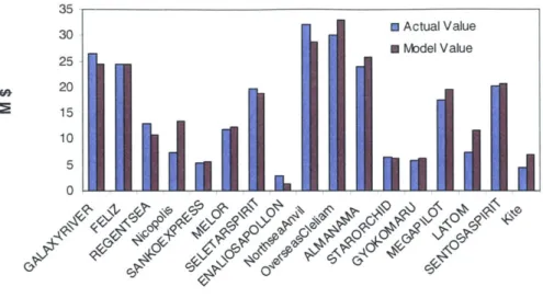
To demonstrate goodness of fit, 60 training cases will be presented in three figures. All the results can be seen in Appendix B. It should be noted that the data listed in the Appendix are in random order.

The next figure shows the results for the first 20 cases of the training set. The actual (desired) value is compared with the model output. According to this figure the model results are adequately close to the desired values.

(30)

Decision Support Tool for the Tanker Second-hand Market Using Data Mining Techniques 35-30 m Actual Value 5 Model Value 25 20 15 10 5 0 0 ' 90

|

?no

9 .

CO4

Figure 6: The Zero Month Model Fit on the first 2OTraining Cases of Tanker Vessels

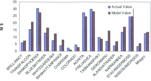
The next figure shows the results for the next 20 cases of the training set.

60 m Actual Value 50 _m_{Mobdel Value} 40 30 20 10 m11i C.,,

Figure 7: The Zero Month Model Fit on the next Training Cases of Tanker Vessels

(31)

The next figure shows the results for the next 20 cases of the training set.

45 40 m Actual Value 35 m lVbdel Value 30 O 25 2 20 15 10 5 0 Il

Figure 8: The Zero Month Model Fit on the next Training Cases of Tanker Vessels

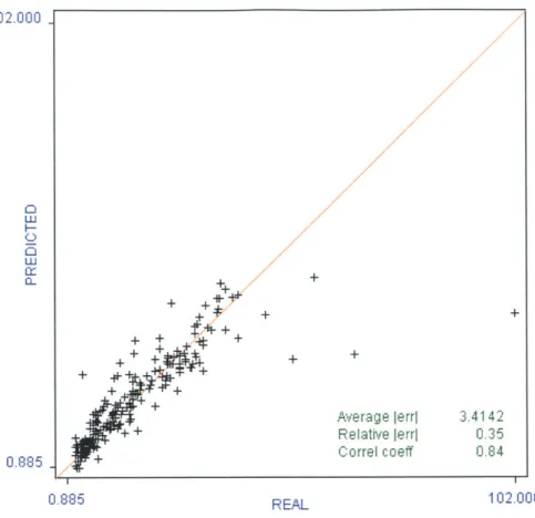
Another way of assessing the accuracy of the predictions is through a visual inspection of a scatter plot that graphs the real target values of the new cases against the values predicted by the model. The scatter plot for training data is shown in figure 9:

(32)

Decision Support Tool for the Tanker Second-hand Market Using Data Mining Techniques 102.000 0/ LU LI C) 0.85. +7 + e off08 ++ + ++ + Average lerrl 3.41 42 +Pelative lerrl 0.35 r orrel coeff 0.84 0.885 REAL 102.000

Figure 9: The Scatter Plot for Zero Month Model Fit on Training Cases of Tanker Vessels

According to the scatter plot the predicted and real numbers for the training process are crosses located around and close to the red line. The red line is the diagonal and shows where the crosses should be located in the non error model. The scope is to construct a model with the crosses of the scatter plot as close to the red line as possible.

The evaluation on test data (200 cases) is shown below: Average lerror 3.8291

Relative

lerrorl

0.38 Correlation coefficient 0.81

To demonstrate goodness of fit 60 testing cases will be presented in three figures. All the results can be seen in Appendix B.

Figure 10 shows the results for the first 20 cases of the testing set. The actual (desired) value is compared with the model output for the test data. According to this figure the results of the model are adequately close to the desired values and show the model's ability to generalize.

(33)

Decision Support Tool for the Tanker Second-hand Market Using Data Mining Techniques 35 m Actual Value 30 2 * Model Value 25 64 20 15 10 5 0

Figure 10: The Zero Month Model Fit on 20 FirstTesting Cases of Tanker Vessels

TFigure bel shows the results for the next 20 cases of the testing set.

40S

30 U Moe Value

40

Fiur 11 Th ZroMothMdel FiVn2 etesigCsso aner esl

Figure 125osterslsfrtenxt2 ae ftetsigst

(34)

Decision Support Tool for the Tanker Second-hand Market Using Data Mining Techniques 35 30 25 20 15 10 5 n m Actual Value m Mbdel Value a~~~Lal C3C 0

Figure 12: The Zero Month Model Fit on 20 NextTesting Cases of Tanker Vessels

The scatter plot for testing data is shown in figure 13:

105.000-n

0.885-0.885 _REAL 105.000

Figure 13: The Scatter Plot for Zero Month Model Fit on Testing Cases of Tanker Vessels

Page 34 of 78 ++ + + + Average lerrI 3.8291 Relative lerr 0.38 Correl coeff 0.81

(35)

According to the scatter plot the vessel cases for the testing process are located around and close to the red line.

Analyzing the results of the Zero Month Model one can say they are adequately acceptable. The error terms are significantly low in all three categories. The Zero Month Model has excellent generalization ability. The error terms in the training (known) data are similar to those in the testing (unknown) data.

3.2 Six Month Model

The six month model is constructed as a useful tool for investors, brokers and ship-owners. The main scope of the model is to provide future estimates for vessel prices according to market states and vessel characteristics. Effort was given in order to model the mechanism that forms future second-hand vessel prices. The time span was set to six months which is a crucial time period when purchasing or selling a vessel. Such a model can be of significant help to a volatile system such as the second-hand market. By studying precedent realization, the six month model has the ability to generalize and predict future vessel prices according to historical records.

3.2.1 Form of the Six Months Model

According to the model's variable definitions, the target attribute was 'Price after six months' which refers to vessel prices after six months.

In the fitting process the tool reads 200 cases from the plus6.data file and 35 attributes from the plus6.names file.

The Six Months Model form has two rules indicating that there are two subgroups where linear equations can be applied. The model is shown below:

Model:

Rule 1: [applying to 82 cases of the training dataset] If

Age > 16

Then

Price after six months = 16.1031 -0.91 [Age]

+ 2.4 [Six previous months moving average of Scrap Value] + 0.0001 [Time Charter Rate]

Rule 2: [applying to 118 cases of the training dataset ]