Prior-based Hierarchical Segmentation Highlighting Structures of Interest

HAL Id: hal-02430333

https://hal.archives-ouvertes.fr/hal-02430333

Submitted on 7 Jan 2020

HAL is a multi-disciplinary open access

archive for the deposit and dissemination of

sci-entific research documents, whether they are

pub-lished or not. The documents may come from

teaching and research institutions in France or

abroad, or from public or private research centers.

L’archive ouverte pluridisciplinaire HAL, est

destinée au dépôt et à la diffusion de documents

scientifiques de niveau recherche, publiés ou non,

émanant des établissements d’enseignement et de

recherche français ou étrangers, des laboratoires

publics ou privés.

Structures of Interest

Amin Fehri, Santiago Velasco-Forero, Fernand Meyer

To cite this version:

Amin Fehri, Santiago Velasco-Forero, Fernand Meyer. Prior-based Hierarchical Segmentation

High-lighting Structures of Interest. Mathematical Morphology - Theory and Applications, De Gruyter

2019, 3, pp.29 - 44. �10.1515/mathm-2019-0002�. �hal-02430333�

Research Article

Open Access

Amin Fehri*, Santiago Velasco-Forero, and Fernand Meyer

Prior-based Hierarchical Segmentation

Highlighting Structures of Interest

https://doi.org/10.1515/mathm-2019-0002

Received March 4, 2019; accepted September 3, 2019

Abstract:Image segmentation is the process of partitioning an image into a set of meaningful regions accord-ing to some criteria. Hierarchical segmentation has emerged as a major trend in this regard as it favors the emergence of important regions at different scales. On the other hand, many methods allow us to have prior information on the position of structures of interest in the images. In this paper, we present a versatile hierar-chical segmentation method that takes into account any prior spatial information and outputs a hierarhierar-chical segmentation that emphasizes the contours or regions of interest while preserving the important structures in the image. Several applications are presented that illustrate the method versatility and efficiency.

Keywords:Mathematical Morphology, Hierarchies, Segmentation, Prior-based Segmentation, Stochastic Wa-tershed.

MSC:06, 68, 94

1 Introduction

In this paper, we propose a method to take advantage of any prior spatial information previously obtained for an image to get a hierarchical segmentation of this image that emphasizes its regions of interest, allowing us to get more details in the designated regions of interest of an image while still preserving its strong structural information. It is an extended version of the conference paper [14].

Image segmentation has been shown to be inherently a multi-scale problem [17]. That is why hierarchical segmentation has become a major trend in image segmentation and most top-performance segmentation techniques [4] [33] [36] [26] [46] [43] fall into this category: hierarchical segmentation does not output a single partition of the image pixels into sets but instead a single multi-scale structure that aims at capturing relevant objects at all scales. Research on this topic is still vivid as differential area profiles [31], robust segmentation of high-dimensional data [16] as well as theoretical aspects regarding the concept of partition lattice [39] [37] and optimal partition in a hierarchy [19] [20] [47]. This paper addresses the problem of developing a hierarchical segmentation algorithm that focuses on certain predetermined zones of the image. The hierarchical aspect also allows us, for tasks previously described, to very simply tune the level of details wanted depending on the application.

Generally, one can use complementary hierarchies to extract pertinent regions in images for given tasks. The idea is then to structure the information present in the image in various controlled ways and use the resulting characterization for segmentation or classification tasks. This information can be complex and is analyzed with discriminative hierarchies regarding the image local content, that is supposed to be distributed homogeneously in the spatial domain. To go further, we show in this paper how to treat images whose content

*Corresponding Author: Amin Fehri:Center of Mathematical Morphology, Mines ParisTech, PSL Research University, E-mail: amin.fehri@mines-paristech.fr

Santiago Velasco-Forero, Fernand Meyer:Center of Mathematical Morphology, Mines ParisTech, PSL Research University, E-mail: santiago.velasco,fernand.meyer@mines-paristech.fr

(a) (b)

(c) (d)

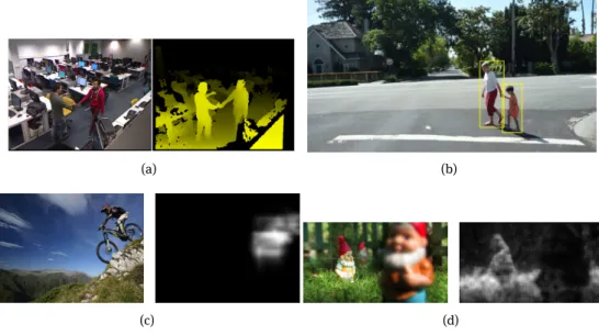
Figure 1: A few examples of the growing number of spatial exogenous information sources: (a) RGBD image, which depth

in-formation can help to direct the segmentation process, (b) many methods provide rough localizations of classes of interests, for example here the class “People”, (c) RGB Image and heatmap of the main class in the image, (d) RGB Image and output of a non-blur zones detector.

How can we use such exogenous information to pilot the hierarchical segmentation process?

is not homogeneously distributed in the spatial domain, and how to take advantage of any prior information over the regions of interests in the images. This way, we can make use of various exogenous spatial infor-mation sources to direct the hierarchical segmentation construction. Such inforinfor-mation can take numerous forms, as illustrated in Figure 1. Indeed, significant developments have been made over the last decades in learning-based recognition methods for various tasks [30] [22] [35]. A variety of sources and modalities have emerged as well, with for example depth sensors [12] or multispectral and hyperspectral cameras [6], and provide additional information that can be useful for segmentation. Having a versatile hierarchical segmen-tation method that can take into account such information during its construction process thus appears to be very interesting. In this regard, our work joins an important research point that consists in designing ap-proaches to incorporate prior knowledge in the segmentation, as shape prior on level sets [5], star-shape prior by graph-cut [44], use of a shape prior hierarchical characterization obtained with deep learning [7], or related work making use of stochastic watershed to perform targeted image segmentation [25].

The stochastic watershed (SWS) consists in an evaluation of an image contours strength by estimating the probability for a contour to appear in the output segmentation when randomly drawing markers in a classical watershed transformation. Building upon the SWS model [3] [26], we propose a method to take advantage of any prior spatial information previously obtained on an image to get a hierarchical segmentation of this image that emphasizes its regions of interest. This allows us to get more details in the designated regions of interest of an image while still preserving its strong structural information. Indeed, we note that such hierarchical clusterings are useful to understand scenes as they enlarge the information support in a controlled way, and hence bring out significant salient features. It has been shown that the SWS model is versatile as multiple construction types can be thought of, the markers we use can be punctual or non-punctual and the number of markers we draw can be changed. In this paper, we go a step further by slightly modifying the SWS model: using a probability density function governing the markers distribution that depends on a spatial exogenous information is a simple yet powerful way to have a very task-adjustable hierarchical segmentation method.

Potential applications are numerous. When having a limited storage capacity (for very large images for example), this would allow us to keep details in the regions of interest as a priority. Similarly, in situations of transmission with limited bandwidth, one could first transmit the important information of the image: the

details of the face for a video-call, the pitch and the players for a soccer game and so on. One could also use such a tool as a preprocessing one, for example to focus on an individual from one camera view to the next one in video surveillance tasks. Finally, from an artistic point of view, the result is interesting and similar to a combination of focus and cartoon effects. Some of these examples are illustrated in this paper.

The remainder of the paper is organized as follows. Section 2 explains how we construct and use graph-based hierarchical segmentation. Then Section 3 specifies how we use prior information on the image to obtain hierarchies with regionalized fineness. Several examples of applications of this method are described in Section 4. Finally, conclusions and perspectives are presented in Section 5.

2 Hierarchies and partitions

2.1 Graph-based hierarchical segmentation

Obtaining a suitable segmentation directly from an image is very difficult. This is why hierarchies are often used to organize and propose interesting contours by valuating them. In this section, we explain how to construct and use graph-based hierarchical segmentations.

For each image, let us suppose that a fine partition is produced by an initial segmentation (for instance a set of superpixels [1] [24] [43], the basins produced by a classical watershed algorithm [27], or a segmen-tation into individual pixels/flat zones) and contains all contours making sense in the image. We define a dissimilarity measure between adjacent tiles of this fine partition. One can then see the image as a graph, the

region adjacency graph(RAG), in which each node represents a tile of the partition; an edge links two nodes if the corresponding regions are neighbors in the image; the weight of the edge is equal to the dissimilarity between these regions. Working on the RAG is much more efficient than working on the image, as there are far less nodes in the RAG than there are pixels in the image. However, this includes a cost regarding the precision of the results.

Formally, we denote this graph G = (V, E, W), where V corresponds to the image domain or set of pix-els/fine regions, E ⊂ V × V is the set of edges linking neighbour regions, W : E → _R+is the dissimilarity measure usually based on local gradient information (or color or texture), for instance W(i, j)∝ |I_{(vi) − I(vj)}|

with I : V→_{R representing the image intensity. Note that this dissimilarity measure ultimately has an}

im-portant impact on the obtained segmentations, and must thus be chosen carefully [32].

The edge linking the nodes p and q is designated by epq. A path is a sequence of nodes and edges: an

example of a path linking the nodes p and s is the set{p_{, e}pt, t, ets, s}. A connected graph is a graph where

each pair of nodes is connected by a path. A cycle is a path whose extremities coincide. A tree is a connected graph without cycle. A spanning tree is a tree containing all nodes. A minimum spanning tree (MST) of a graph G, hereafter called MST(G), is a spanning tree with minimal possible weight (the weight of a tree being equal to the sum of the weights of its edges), obtained for example using the Jarník’s algorithm [18] (later rediscovered by Prim, and thus often also known as the Prim’s algorithm [34]). A forest is a collection of trees. A partition

π_{of a set V is a collection of subsets of V, such that the whole set V is the disjoint union of the subsets in the}

partition, i.e., π ={R₁, R2, . . . , Rk}, such that∀i, Ri⊆V ;∀i≠ j, Ri∩Rj=∅;⋃︀kiRi= V.

Cutting all edges of the MST(G) having a valuation superior to a threshold λ leads to a minimum spanning forest (MSF) F(G, λ), i.e. to a partition of the graph. Note that the obtained partition is the same that one would have obtained by cutting edges superior to λ directly on G [29]. Since working on the MST(G) is less costly and provides similar results regarding graph-based segmentation, we work only with the MST(G) in the remainder of this paper.

So cutting edges by decreasing valuations gives an indexed hierarchy of partitions (H, λ), with H a

hierar-chy of partitions_{i.e. a chain of nested partitions H =}{π_{0, π1, . . . , π}n|∀j, k, 0 ≤ j ≤ k ≤ n⇒πj⊑πk}, with

πnthe single-region partition and π₀the finest partition on the image, and λ : H→R+being a stratification index verifying λ(π) < λ(π′) for two nested partitions π ⊂ π′_{. This increasing map allows us to value each}

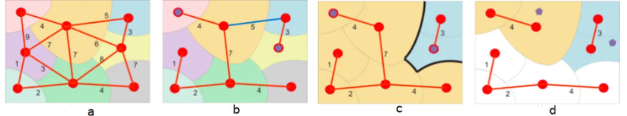
Figure 2: a: A partition represented by an edge-weighed graph. b: A minimum spanning tree of the graph, with 2 markers in

blue: the highlighted edge in blue is the highest edge on the path linking the two markers.c: The segmentation obtained when

cutting this edge.d: Blue and orange domain are the domains of variation of the two markers generating the same

segmenta-tion.

we consider that the higher the saliency, the stronger the contour. For a given hierarchy, the image in which each contour takes as value its saliency is called Ultrametric Contour Map (UCM) [4]. It is also referred to as a

saliency map_{in the literature [9] [10]. Representing a hierarchy by its UCM is an easy way to get an idea of its}

effect because thresholding an UCM always provides a set of closed curves and so a partition. In this paper, for better visibility, we represent UCM with inverted contrast.

To get a partition for a given hierarchy, there are several possibilities: – simply thresholding the highest saliency values,

– marking some nodes as important ones and then computing a partition accordingly, which is known as marker-based segmentation [28],

– smartly editing the graph by finding the partition that minimizes an energy function [17] [20] [47]. In a complementary approach, we argue that the quality of the obtained partitions highly depends on the dissimilarity that we use, and thus that changing the dissimilarity can lead to more suitable partitions [13]. Indeed, if the dissimilarity reflects only a local contrast as in the hierarchy issued by the RAG, the most salient regions in the image are the small contrasted ones. So instead of departing from a simple and rough dissimilarity such as contrast and then use a sophisticated technique to get a good partition out of it, one can also try to obtain a more informative dissimilarity adapted to the content of the image such that the sim-plest methods are sufficient to compute interesting partitions. This way, the aforementioned techniques lead to segmentations better suited for further exploitation. How can we construct more pertinent and informa-tive dissimilarities? One possible way to do so is by using stochastic watershed hierarchies, that we hereby introduce.

2.2 Stochastic watershed hierarchies

The stochastic watershed (SWS), introduced in [3] on a simulation basis and extended with a graph-based approach in [26], is a versatile tool to construct hierarchies. The seminal idea is to perform marker-based segmentation multiple times with random markers and weight each edge of the MST by its frequency of appearance in the resulting segmentations.

Indeed, by spreading markers on the RAG G, one can construct a segmentation as a MSF F(G) in which each tree takes root in a marked node. Marker-based segmentation directly on the MST is possible: one must then cut, for each pair of markers, the highest edge on the path linking them (its value corresponding to the ultrametric distance between these marked nodes). Furthermore, there is a domain of variation in which each marker can move while still leading to the same final segmentation. More details are provided in Figure 2.

Let us then consider on the MST an edge estof weight ωstand compute its probability to be cut. We cut

all edges of the MST with a weight superior or equal to ωst, producing two trees Tsand Ttwith roots s and t.

If at least one marker falls within the domain Rsof Tsnodes and at least one marker falls within the domain

Let µ(R) denote the number of random markers falling in a region R. We want to attribute to estthe

fol-lowing probability value:

P[(µ(Rs) ≥ 1)∧(µ(Rt) ≥ 1)] = 1 − P[(µ(Rs) = 0)∨(µ(Rt) = 0)]

= 1 − P(µ(Rs) = 0) − P(µ(Rt) = 0) + P(µ(Rs∪Rt) = 0).

(1) If markers are spread following a Poisson distribution, then for a region R:

P(µ(R) = 0) = exp−Γ(R), (2) with Γ(R) being the expected value (mean value) of the number of markers falling in R. The probability thus becomes:

P(µ(Rs) ≥ 1∧µ(Rt) ≥ 1) = 1 − exp−Γ(Rs)− exp−Γ(Rt)+ exp−Γ(Rs∪Rt). (3)

When the Poisson distribution has an homogeneous density𝛾, the expected value of the number of markers falling in R can be expressed as:

Γ(R) = area(R)𝛾. (4) But when the Poisson distribution has a non-uniform density𝛾, its expression becomes:

Γ_{(R) =}

∫︁

(x,y)∈R

𝛾_{(x, y) dxdy. (5)}

Thus, the output of the SWS algorithm depends on the MST (structure and edges valuations) and the probabilistic law governing markers distribution. Furthermore, SWS hierarchies can be chained, leading to a wide exploratory space that can be used in a segmentation workflow [13].

Because of its versatility and good performance, SWS represents a method of choice for introducing prior information into a segmentation workflow. Indeed, when having a prior information about the image, it is possible to use it in order to have more details in some parts rather than others.

3 Hierarchies highlighthing structures of interest using prior

information

3.1 Hierarchy with Regionalized Fineness (HRF)

In the original SWS, a uniform distribution of markers is used (whatever size or form they may have). In order to have stronger contours in a specific region of the image, we adapt the model so that more markers are spread in this region.

Let E be an object or class of interest, for example E = “face of a person”, and I be the studied image. We denote by θEthe probability density function (PDF) associated with E obtained separately, and defined on the

domain D of I, and by PM(I, θE) the associated probabilistic map, in which each pixel p(x, y) of I takes as value

θE(x, y), its probability to be part of E. Such a PDF can be obtained using any of the numerous methods from

various scientific fields to spatially characterize an image, as illustrated in Figure 1. Given such information on the position of an event in an image, we obtain a hierarchical segmentation focused on this region by modulating the distribution of markers. We call this structure a Hierarchy with Regionalized Fineness (HRF), as it features more details within the region of interest. We compute it by modifying the law governing the distribution of markers in the SWS algorithm, for it to take into account the spatial information provided by the PDF associated with the object of interest. If𝛾_{is a density defined on D to distribute markers (uniform or}

not), we set θE𝛾as a new density, thus favoring the emergence of contours within the regions of interest.

Considering a region R of the image, and taking as a new density θE𝛾to direct the distribution of markers

within the region of interest, the mean number of markers falling within R becomes:

Γ_{E(R) =}

∫︁

(x,y)∈R

Furthermore, since the number of markers falling within each region has an influence on the new edge weights that are computed, it is interesting to control this number of markers to constrain the edge weights to lie within a reasonable value range and thus avoid numerical issues (with values becoming too small for example). This is possible by modifying this model. If we want N markers to fall in average within the domain

D, we can thus work with a slightly modified density, by multiplying the density by N and dividing it by the expected value of the number of markers falling in D:

^

𝛾₌ N

Γ_(D)𝛾. (7)

Furthermore, this approach can be easily extended to the case where we want to take advantage of infor-mation from multiple sources. Indeed, if θE1and θE2 are the PDF associated with two events E1and E2, we

can for example combine those two sources by using as a new density (θE1× θE2)𝛾. This corresponds to a new

event{E₁AND E2}.

3.2 Methodology

In this section, we present the steps to compute a HRF for an event E given a probabilistic map PM(I, θE)

providing spatial prior information on an image I:

1. compute a fine partition π0of the image, define a dissimilarity measure between adjacent regions and

the RAG G, as illustrated in Figures 3(a)(b)(c),

2. compute MST(G), and a new probabilistic map ̃︁PM(π0, I, θE) with each region of the fine partition π0

taking as a new value the mean value of PM(I, θE) in each region, as shown in Figures 3(d)(e)(f),

3. compute new values of edges using the method described in Section 3.1, where for each region Riof π0,

Γ_{(Ri) corresponds to the mean value taken by pixels of the region Riin ̃︁PM(π0, I, θE). Note that this}

ap-proach allows a highly efficient implementation using dynamic programming on graphs. The resulting hierarchy retains more details in the region of interest, while still capturing the important structures of the image, as one can see on an example in Figures 3(g)(h)(i).

(a) (b) (c)

(d) (e) (f)

(g) (h) (i)

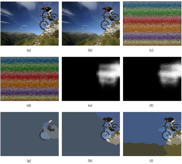
Figure 3: Illustration of the methodology described in Section 3.2 to generate a hierarchy with regionalized fineness. (a) Image I. (b) π₀visualized by the mean value per region on I. (c) RAG_{G, superimposed on a label image with fake colors of the fine} segmentation for better visualization. (d)MST(G) (same visualization as in (c)). (e) Probabilistic Map PM(I, θE)) associated with

“Bike” class. (f) ̃︁PM(π0, I, θE). (g)(h)(i) examples of segmentations obtained with HRF - 10, 100, 200 regions.

Making use of multiple sources is also very simple and consists in fusing the probability maps in a con-trolled way, depending on the objective. It will be illustrated in Figure 6.

3.3 Modulating the HRF depending on the pairs of regions considered

If we want to favor certain contours to the detriment of others, we can modulate the density of markers in each region by taking into account the strength of the contour separating them but also the relative position of both regions.

We use the same example and notations as in Section 3.1, and thus modulate the distribution of markers relatively to Rs, Rtand their frontier. For example, to stress the strength of the gradient separating both regions

we can locally spread markers following the distribution χ(Rs, Rt)𝛾, with χ(Rs, Rt) = ωst. This corresponds to

the classical volume-based SWS [42], which allows to obtain a hierarchy that takes into account both surfaces of regions and contrast between them.

(a) (b) (c) (d)

(e) (f) (g)

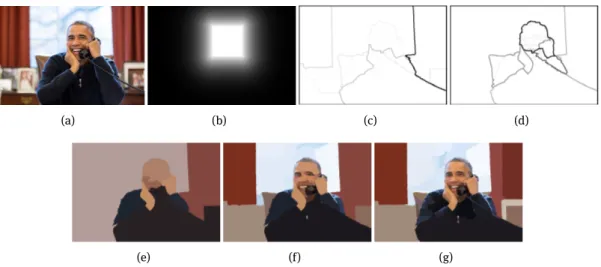
Figure 4: Hierarchical segmentation of faces. (a) Original image. (b) Prior: Probabilistic map obtained thanks to a face detection

algorithm. (c) Volume-based SWS Hierarchy UCM. (d) Volume-based HRF UCM with face position as prior. (e)(f)(g) Examples of segmentations obtained with HRF - 10,100,1000 regions.

To go further, one can use any prior information in a similar way. Indeed, while using prior information to influence the output of the segmentation workflow, one might also want to choose whether the relevant information to emphasize in resulting segmentations is the foreground, the background or the transitions between them.

For example, having more details in the transition regions between background and foreground allows us to have more precision where the limit between foreground and background is actually unclear. As a matter of fact, the prior information often only provides rough positions of the foreground object with blurry contours, and such a process would allow to get precise contours of this object from the image.

Let us consider this case and define for each couple of regions (Rs, Rt) a suitable χ(Rs, Rt). We then want

χ(Rs, Rt) to be low if Rsand Rtboth are in the background or the foreground, and high if Rsis the background

and Rtin the foreground (or the opposite). We use:

˜

𝛾= χ𝛾, with χ(Rs, Rt) = max(m(Rs), m(Rt))(1 − min(m(Rs), m(Rt)))

0.01 + σ(Rs)σ(Rt) , (8)

m_{(R) (resp. σ(R)) being the normalized mean (resp. normalized standard deviation) of pixels values in the}

region R of PM(I). Thus the number of markers spread will be higher when the contrast between adjacent regions is high (numerator term) and when these regions are coherent (denominator term). Then for each edge, its new probability to be cut is:

P[(µ(Rs) ≥ 1)∧(µ(Rt) ≥ 1)] = 1 − exp−χ(Rs,Rt)Γ(Rs)− exp−χ(Rs,Rt)Γ(Rt)

+ exp−χ(Rs,Rt)Γ(Rs∪Rt) (9)

In the spirit of [8] [2], this mechanism provides us with a way to “realign” the hierarchy with respect to the relevant prior information to get more details where the information is blurry. Similar adaptations can be thought of to emphasize details of background or foreground regions. In the following, we illustrate the methodology with some application examples.

4 Application examples

4.1 Scalable transmission favoring regions of interest

Let us consider a situation where one emitter wants to transmit an image through a channel with a limited bandwidth, e.g. for a videoconference call. In such a case, the more important information to transmit are details on the face of the person on the image. Besides, we nowadays have highly efficient face detectors, using for example Haar-wavelets as features in a learning-based vision approach [45]. Considering that for an input image, the face can be easily detected, we can use this information to produce a hierarchical segmentation of the image that accentuates the details around the face while giving a good sketch of the image elsewhere. Depending on the bandwidth available, we can then choose the level of the hierarchy to select and obtain the associated partition to transmit, ensuring us to convey the face with as much details as possible. Some results are presented in Figure 4, with notably a comparison between a classical volume-based SWS UCM and a volume-based HRF UCM.

The same method can also be used for artistic purposes. For example, when taking as prior the result of a blur detector [41], we can accentuate the focus effect wanted by the photograph and turn it into a cartoon effect as well - see Figure 5 for an illustration of the results.

(a) (b) (c) (d)

(e) (f) (g)

Figure 5: Hierarchical segmentation of non-blur objects. (a) Original image. (b) Prior image obtained with non-blur zones

de-tection algorithm. (c) Volume-based SWS Hierarchy UCM. (d) Volume-based HRF UCM with non-blur zones as prior. (e)(f)(g) Examples of segmentations obtained with HRF - 10,200,2000 regions.

4.2 Building a HRF using different sources

One can as well build hierarchies obtained with prior information coming from multiple sources. Let us con-sider for example a RGB-D image in which a person is present. A face detection algorithm can be used to localize the face of the person in the image. Using this information, one can then extract the particular depth at which the face of the person (and thus the person in most cases) is present in the depth image.

One thus obtains two probability maps: one associated with the face of the person, that we denote PMF,

the other translating the depth at which the person is, that we denote PMD. Combining these two probability

maps by multiplying them (which corresponds to the logical operator AND) then leads to a new probability map PMAND(F,D)that highlights the whole body of the person with a particular emphasis on his face, as one

can see in Figure 6.

The HRF HAND(F,D)built using PMAND(F,D)better captures the pertinent information than the two HRF HF

by comparing Figures 6(b), 6(f) and 6(j) that the hair of the person appear sooner in the latter than in the two former, while still retaining details regarding the depth at which the person is, such as the structure of the t-shirt or the legs.

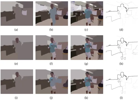
Figure 6: Example of the combination of two probability maps to get a new one that can be put as input of the HRF. We have

two probability maps, θFhighlighting the face, and θDcorresponding to the specific depth at which the character is. We use

(θF× θD)𝛾 as a new probability density function.

(a) (b) (c) (d)

(e) (f) (g) (h)

(i) (j) (k) (l)

Figure 7: Example of the effect of the combination of probability maps for HRF.PMFis associated with the face,PMDwith the

specific depth at which the character is,PMAND(F,D)= PMD× PMDwith their logical AND combination.

(a)(b)(c)HFsegmentation examples: 5, 25, 100 regions. (d)HFUCM. (e)(f)(g)HDsegmentation examples: 5, 25, 100 regions.

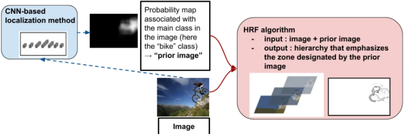
Figure 8: Proposed workflow of weakly-supervised HRF algorithm.

4.3 Weakly-supervised HRF

In the same spirit, various methods now exist to automatically roughly localize the principal object in an image. We inspire ourselves from [30] to do so. Using a deep convolutional neural network (CNN) classifier VGG19 [40] trained on the 1000 classes of the ImageNet database [11], we first determine what is the main class in the image. Note that this CNN takes as input only images of size 224 × 224 pixels. Once it is known, we can then, by rescaling the image by a factor s∈ {0.5, 0.7, 1.0, 1.4, 2.0, 2.8}(as suggested in [30]), compute for sub-windows of size 224 × 224 of the image the probability of appearance of the main class. By simply superimposing the results for all sub-windows, we thus obtain a probabilistic map of the main class for each rescaling factor. By max-pooling, we keep in memory the result of the scale for which the probability is the highest. The heatmap thus generated takes as value in each pixel the probability that this pixel belongs to the class of interest. This probability map can then be used to feed our algorithm. This way, we have at our disposal an automatized way to focus on the principal class in the scene with the desired level of detail.

All in all, the combination of this approach and the HRF is very interesting as it constitutes an all-in-one method to classify the image (i.e. to find the main class in the image), to localize the objects of this main class in it, and to get from it a hierarchy of segmentation in which those elements are highlighted. An overview of this method can be found in Figure 8 and an example is presented in Figure 9, for the same image as in Figure 3 from Section 3.2.

(a) (b)

Figure 9: Hierarchical segmentation of the main class (class “bike”) in an image with heatmap issued of a CNN-based method

4.4 Hierarchical co-segmentation

Another potential application is to co-segment with the same fineness level an object appearing in several different images. For example, when given a list of images of the same object taken from different perspec-tives/for different conditions, we can follow one of the state-of-the-art matching procedure [23] (the reader is referred to [48] for a thorough evaluation of the instance retrieval methods, which is beyond the scope of this paper):

1. compute all key-points in all images, using for example the FAST algorithm [38], 2. find local descriptors at these key-points, such as SIFT [23],

3. match those key-points using a spatial coherency algorithm as RANSAC [15].

Once it is done we retain these matched key-points between all images, and generate probability maps of the appearance of the matched objects using a morphological distance function to the matched key-points.

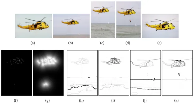
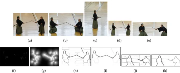
These probability maps can then feed our algorithm, resulting in a hierarchical co-segmentation that emphasizes the matched zones of the image. Some results are presented in Figures 10 and 11, which speak for the interest of such an approach. In Figure 10, while the contours/details in the helicopter are not necessarily the more salient ones in each image taken separately, the matching of keypoints throughout images results in a prior image emphasizing regions inside it. The comparison of the volume-based SWS hierarchy and HRF saliency maps confirms that the details in the helicopter are much more efficiently highlighted in the latter. In the same way, in Figure 11, the details in the HRF UCM in Figures 11(i),(k) are way more focused on the kendoka (kendo practitioners) than on the comparison UCM in Figures 11(h),(j). The process thus helps us obtaining representations of images emphasizing shared objects between them, and with the desired level of detail. Note that such a method could highly benefit approaches making use of hierarchical segmentation for co-saliency detection such as [21], by producing hierarchical segmentations that already retain contours of shared objects between images, in a robust manner (since the keypoints and descriptors used are robust to image transformation, occlusions etc.).

(a) (b) (c) (d) (e)

(f) (g) (h) (i) (j) (k)

Figure 10: Hierarchical co-segmentation of matched objects - example 1. (a)-(e) I1to I5. (f) All matched key-points of I3with other images key-points. (g) Prior for I₃: probability map generated thanks to morphological distance function. (h) Volume-based SWS Hierarchy UCM for I₃. (i) Volume-based HRF UCM for I₃with matched key-points as prior. (j) Volume-based SWS Hierarchy UCM for I₄. (k) Volume-based HRF UCM for I₄with matched key-points as prior.

(a) (b) (c) (d) (e)

(f) (g) (h) (i) (j) (k)

Figure 11: Hierarchical co-segmentation of matched objects - example 2. (a)-(e) I1to I5(f) All matched key-points of I2with other images key-points. (g) Prior for I2: probability map generated thanks to morphological distance function. (h) Volume-based SWS Hierarchy UCM for I₂. (i) Volume-based HRF UCM for I₂with matched key-points as prior. (j) Volume-based SWS Hierarchy UCM for I5(k) Volume-based HRF UCM for I5with matched key-points as prior.

4.5 Effect of the HRF highlighting transitions between foreground and background

We illustrate in this section the HRF highlighting transitions between foreground and background presented in Section 3.3. We present its effect in the weakly-supervised HRF example in Figure 12, and in the face detec-tion example in Figure 13. One can notice that insisting on the transidetec-tion between background and foregroud helps to better delineate the contours corresponding to these transitions in both examples. In Figure 13(j), we thus observe how the hands and face of the character emerge first. Similarly, in Figure 12(e)(f), we see that the car structure emerges in early levels of the hierarchy, whereas we do not obtain such a result otherwise.

(a) (b) (c) (d)

(e) (f) (g) (h)

Figure 12: Hierarchical segmentation of the main class in the image (class “car”) highlighting transitions between background

and foreground. (a) Image. (b) Heatmap of the class “car”. Case 1: HRF (c) UCM. (e) 5 regions. (f) 10 regions.

(a) (b) (c)

(d) (e) (f)

(g) (h) (i)

(j) (k) (l)

Figure 13: Hierarchical segmentation of faces highlighting transitions between background and foreground.

Case 1: HRF depending on the couples of regions (Section 3.3) (a) UCM. (d) 4 regions. (e) 10 regions. (f) 25 regions. Case 2: HRF depending on the regions only (Section 3.1) (b) UCM. (g) 4 regions. (h) 10 regions. (i) 25 regions. Case 3: Both combined (c) UCM. (j) 4 regions. (k) 10 regions. (l) 25 regions.

5 Conclusions and perspectives

In this paper we have proposed a novel and efficient hierarchical segmentation algorithm that emphasizes the regions of interest in the image by using spatial exogenous information on it. The wide variety of sources for this exogenous information makes our method extremely versatile and its potential applications numerous, as shown by the examples developed in the last section. To go further, we could find a way to efficiently extend this work to videos. One could also imagine a semantic segmentation method that would go back and forth between localization algorithm and HRF to progressively refine the contours of the main objects in the image.

References

[1] Achanta, R., Shaji, A., Smith, K., Lucchi, A., Fua, P., Süsstrunk, S.: Slic superpixels compared to state-of-the-art superpixel methods. IEEE transactions on pattern analysis and machine intelligence 34(11), 2274–2282 (2012)

[2] Adão, M.M., Guimarães, S.J.F., Patrocínio, Z.K.: Evaluation of scale-aware realignments of hierarchical image segmentation. In: Iberoamerican Congress on Pattern Recognition. pp. 141–149. Springer (2018)

[3] Angulo, J., Jeulin, D.: Stochastic watershed segmentation. ISMM 1, 265–276 (2007)

[4] Arbelaez, P., Maire, M., Fowlkes, C., Malik, J.: Contour detection and hierarchical image segmentation. IEEE PAMI 33(5), 898–916 (2011)

[5] Chan, T., Zhu, W.: Level set based shape prior segmentation. In: CVPR. vol. 2, pp. 1164–1170 (2005)

[6] Chang, C.I.: Hyperspectral imaging: techniques for spectral detection and classification, vol. 1. Springer Science & Business Media (2003)

[7] Chen, F., Yu, H., Hu, R., Zeng, X.: Deep learning shape priors for object segmentation. In: CVPR. pp. 1870–1877 (2013) [8] Chen, Y., Dai, D., Pont-Tuset, J., Van Gool, L.: Scale-aware alignment of hierarchical image segmentation. In: Proceedings of

the IEEE Conference on Computer Vision and Pattern Recognition. pp. 364–372 (2016)

[9] Cousty, J., Najman, L.: Incremental algorithm for hierarchical minimum spanning forests and saliency of watershed cuts. In: International Symposium on Mathematical Morphology and Its Applications to Signal and Image Processing. pp. 272–283. Springer (2011)

[10] Cousty, J., Najman, L., Kenmochi, Y., Guimarães, S.: Hierarchical segmentations with graphs: quasi-flat zones, minimum spanning trees, and saliency maps. Journal of Mathematical Imaging and Vision 60(4), 479–502 (2018)

[11] Deng, J., Dong, W., Socher, R., Li, L.J., Li, K., Fei-Fei, L.: Imagenet: A large-scale hierarchical image database. In: 2009 IEEE conference on computer vision and pattern recognition. pp. 248–255. IEEE (2009)

[12] Fankhauser, P., Bloesch, M., Rodriguez, D., Kaestner, R., Hutter, M., Siegwart, R.: Kinect v2 for mobile robot navigation: Evaluation and modeling. In: Advanced Robotics (ICAR), 2015 International Conference on. pp. 388–394. IEEE (2015) [13] Fehri, A., Velasco-Forero, S., Meyer, F.: Automatic selection of stochastic watershed hierarchies. In: 2016 24th European

Signal Processing Conference (EUSIPCO). pp. 1877–1881. IEEE (2016)

[14] Fehri, A., Velasco-Forero, S., Meyer, F.: Prior-based hierarchical segmentation highlighting structures of interest. In: Interna-tional Symposium on Mathematical Morphology and Its Applications to Signal and Image Processing. pp. 146–158. Springer (2017)

[15] Fischler, M.A., Bolles, R.C.: Random sample consensus: a paradigm for model fitting with applications to image analysis and automated cartography. In: Readings in computer vision, pp. 726–740. Elsevier (1987)

[16] Gueguen, L., Velasco-Forero, S., Soille, P.: Local mutual information for dissimilarity-based image segmentation. JMIV pp. 1–20 (2013)

[17] Guigues, L., Cocquerez, J.P., Le Men, H.: Scale-sets image analysis. IJCV 68(3), 289–317 (2006) [18] Jarník, V.: O jistém problému minimálním.(z dopisu panu o. borůvkovi)

[19] Kiran, B.R., Serra, J.: Ground truth energies for hierarchies of segmentations. In: ISMM, pp. 123–134 (2013)

[20] Kiran, B.R., Serra, J.: Global-local optimizations by hierarchical cuts and climbing energies. Pattern Recognition 47(1), 12–24 (2014)

[21] Liu, Z., Zou, W., Li, L., Shen, L., Le Meur, O.: Co-saliency detection based on hierarchical segmentation. IEEE Signal Process-ing Letters 21(1), 88–92 (2014)

[22] Long, J., Shelhamer, E., Darrell, T.: Fully convolutional networks for semantic segmentation. In: Proceedings of the IEEE conference on computer vision and pattern recognition. pp. 3431–3440 (2015)

[23] Lowe, D.G.: Distinctive image features from scale-invariant keypoints. IJCV 60(2), 91–110 (2004)

[24] Machairas, V., Faessel, M., Cárdenas-Peña, D., Chabardes, T., Walter, T., Decencière, E.: Waterpixels. IEEE TIP 24(11), 3707– 3716 (2015)

[25] Malmberg, F., Hendriks, C.L.L., Strand, R.: Exact evaluation of targeted stochastic watershed cuts. Discrete Applied Mathe-matics 216, 449–460 (2017)

[26] Meyer, F.: Stochastic watershed hierarchies. In: ICAPR. pp. 1–8 (2015)

[27] Meyer, F., Beucher, S.: Morphological segmentation. Journal of visual communication and image representation 1(1), 21–46 (1990)

[28] Meyer, F.: Minimum spanning forests for morphological segmentation. In: Mathematical morphology and its applications to image processing, pp. 77–84. Springer (1994)

[29] Najman, L., Cousty, J., Perret, B.: Playing with kruskal: algorithms for morphological trees in edge-weighted graphs. In: Mathematical Morphology and Its Applications to Signal and Image Processing, pp. 135–146. Springer (2013)

[30] Oquab, M., Bottou, L., Laptev, I., Sivic, J.: Is object localization for free?-weakly-supervised learning with convolutional neural networks. In: Proceedings of the IEEE Conference on Computer Vision and Pattern Recognition. pp. 685–694 (2015) [31] Ouzounis, G.K., Pesaresi, M., Soille, P.: Differential area profiles: decomposition properties and eflcient computation. IEEE

PAMI 34(8), 1533–1548 (2012)

[32] Perret, B., Cousty, J., Guimaraes, S.J.F., Maia, D.S.: Evaluation of hierarchical watersheds. IEEE Transactions on Image Pro-cessing 27(4), 1676–1688 (2018)

[33] Pont-Tuset, J., Arbelaez, P., Barron, J.T., Marques, F., Malik, J.: Multiscale combinatorial grouping for image segmentation and object proposal generation. IEEE transactions on pattern analysis and machine intelligence 39(1), 128–140 (2016) [34] Prim, R.C.: Shortest connection networks and some generalizations. The Bell System Technical Journal 36(6), 1389–1401

(1957)

[35] Redmon, J., Divvala, S., Girshick, R., Farhadi, A.: You only look once: Unified, real-time object detection. In: Proceedings of the IEEE conference on computer vision and pattern recognition. pp. 779–788 (2016)

[36] Ren, Z., Shakhnarovich, G.: Image segmentation by cascaded region agglomeration. In: CVPR. pp. 2011–2018 (2013) [37] Ronse, C.: Ordering partial partitions for image segmentation and filtering: Merging, creating and inflating blocks. JMIV pp.

1–32 (2013)

[38] Rosten, E., Drummond, T.: Machine learning for high-speed corner detection. In: European conference on computer vision. pp. 430–443. Springer (2006)

[39] Serra, J.: Tutorial on connective morphology. Selected Topics in Signal Processing, IEEE Journal of 6(7), 739–752 (Nov 2012) [40] Simonyan, K., Zisserman, A.: Very deep convolutional networks for large-scale image recognition. arXiv 1409.1556 (2014) [41] Su, B., Lu, S., Tan, C.L.: Blurred image region detection and classification. In: ACM International Conference on Multimedia.

pp. 1397–1400. MM ’11 (2011)

[42] Vachier, C., Meyer, F.: Extinction value: a new measurement of persistence. In: IEEE Workshop on nonlinear signal and image processing. vol. 1, pp. 254–257 (1995)

[43] Vargas-Muñoz, J.E., Chowdhury, A.S., Alexandre, E.B., Galvão, F.L., Miranda, P.A.V., Falcão, A.X.: An iterative spanning forest framework for superpixel segmentation. IEEE Transactions on Image Processing 28(7), 3477–3489 (2019)

[44] Veksler, O.: Star shape prior for graph-cut image segmentation. In: ECCV, pp. 454–467. Springer (2008)

[45] Viola, P., Jones, M.: Rapid object detection using a boosted cascade of simple features. In: CVPR. pp. 511–518 (2001) [46] Wei, X., Yang, Q., Gong, Y., Ahuja, N., Yang, M.H.: Superpixel hierarchy. IEEE Transactions on Image Processing 27(10), 4838–

4849 (2018)

[47] Xu, Y., Géraud, T., Najman, L.: Hierarchical image simplification and segmentation based on mumford-shah-salient level line selection. Pattern Recognition Letters (2016)

[48] Zheng, L., Yang, Y., Tian, Q.: Sift meets cnn: A decade survey of instance retrieval. IEEE transactions on pattern analysis and machine intelligence 40(5), 1224–1244 (2017)