Étude sur l'observabilité de l'atmosphère et l'impact des observations sur les prévisions météorologiques

ÉTUDE SUR L'OBSERVABILITÉ DE L'ATMOSPHÈRE ET L'IMPACT DES OBSERV ATIONS SUR LES PRÉVISIONS MÉTÉOROLOGIQUES

THÈSE

PRÉSENTÉE

COMME EXIGENCE PARTIELLE

DU DOCTORAT EN SCIENCES DE L'ENVIRONNEMENT

PAR CRISTINA LUPU

Service des bibliothèques

Avertissement

La diffusion de cette thèse se fait dans le respect des droits de son auteur, qui a signé le formulaire Autorisation de reproduire et de diffuser un travail de recherche de cycles supérieurs (SDU-522 - Rév.ü1-2üü6). Cette autorisation stipule que «conformément

à

l'article 11 du Règlement no 8 des études de cycles supérieurs, [l'auteur] concède

à

l'Université du Québec

à

Montréal une licence non exclusive d'utilisation et de publication de la totalité ou d'une partie importante de [son] travail de recherche pour des fins pédagogiques et non commerciales. Plus précisément, [l'auteur] autorise l'Université du Québec

à

Montréal

à

reproduire, diffuser, prêter, distribuer ou vendre des copies de [son] travail de recherche

à

des fins non commerciales sur quelque support que ce soit, y compris l'Internet. Cette licence et cette autorisation n'entraînent pas une renonciation de [la] part [de l'auteur] à [ses] droits moraux ni à [ses] droits de propriété intellectuelle. Sauf entente contraire, [l'auteur] conserve la liberté de diffuser et de commercialiser ou non ce travail dont [il] possède un exemplaire.»

Cette thèse est le résultat de quatre années de travail à l'Université du Québec à Montréal. Je tiens remercier ici très chaleureusement toutes les personnes avec qui j'ai partagé cette période.

En premier lieu, je tiens à exprimer toute ma gratitude au Prof. Pierre Gauthier pour avoir encadré ma thèse. Les innombrables discussions que nous avons eues au cours de cette thèse m'ont permis d'apprécier son expertise en assimilation de données, son enthousiasme communicatif et son ouvelture d'esprit. Je le remercie pour ses conseils avisés, pour sa disponibilité permanente et pour ses encouragements dans des moments difficiles tout au long de ces années. Un merci particulier pour avoir soigneusement corrigé mes textes et pour m'avoir appris la rédaction d'un texte scientifique.

Je tiens à remercier également les membres de mon comité de thèse, Messieurs Jean­ PielTe Blanchet et Louis Garand, d'avoir contribué à l'encadrement de ma recherche de doctorat. Je tiens d'autre part à remercier les membres de la Division d'assimilation de données et de météorologie satellitaire d'Environnement Canada pour les échanges scientifiques, techniques et informatiques. Stéphane Laroche, Mark Buehner, Monique Tanguay, Jean-François Caron, Ahmed Mahidjiba, Pierre Koclas et Simon Pellerin m'ont apporté une aide précieuse. Merci également aux membres du Service Informatique à Dorval pour leur support et coopération.

Je tiens à remercier également les membres du jury qui ont accepté de réviser ma thèse. Merci au Prof. René Laprise d'avoir accepté de présider le jury de cette thèse, au Dr. Carla Cardinali, au Dr. Mark Buehner, et au Prof. Pierre Gauthier pour avoir accepté d'évaluer mon travail de thèse. Leurs remarques et recommandations m'ont permis d'apporter des améliorations à la version finale de la thèse.

Plus largement, ma reconnaissance va aussi à toute l'équipe du centre ESCER/UQAM: professeurs, collègues, personnel administratif et technique. Une pensée particulière à mon compagnon de bureau et ami Alexandru Stefanof, véritable encyclopédie vivante. Je le remercie pour ses encouragements et pour tout ce que j'ai appris lors de nos conversations quotidiennes. Je remercie aussi Emilia Diaconescu, DOl'ina Surcel, Cristina Stefanof, Ana

Berbeleac pour le soutien appolié tout au long de ma thèse et pour les bons moments passés ensemble au travail et en dehors.

Un merci tout particulier et chaleureux à mon mari, Gheorghe Milea, qui m'a soutenu toutes ces années et m'a donné la force et la motivation nécessaires pour temliner. Ce travail est aussi le résultat de son soutien et de sa confiance. Merci également à mes chers parents et à mon frère pour leurs encouragements.

LISTE DES FIGURES vii

LISTE DES TABLEAUX ix

LISTE DE SIGLES ET ACRONYMES xi

LISTE DES SYMBOLES xiii

RÉSUMÉ xvii

INTRODUCTION 1

CHAPITRE II

OBSERV ABILITÉ DES FONCTIONS DE STRUCTURE DÉPENDANTES DE

L'ÉCOULEMENT POUR UTILISATION EN ASSIMILATION DE DONNÉES 11

2.1 Introduction 14

2.2 Flow-dependent structure functions in 3D-Var: the adapted 3D-Var 17

2.2.1 3D variational assimilation 17

2.2.2 Adapted 3D-Var approach 18

2.3 Assimilation in the subspace sparmed by sensitivities 20 2.3.1 Use of a B matrix confined within the subspace spanned by

a single sensitive direction 20

2.3.2 Observability of a pelturbatiol1 stlUcture 22

2.4 Example based on 1D-Var expeliments 22

2.5 Results with 3D-Var using different definitions for the stIllcture functions 25

2.5.1 A test case 27

2.5.2 Application in an adapted 3D-Var context 28

2.5.3 Experiments with a pseudo-inverse defined in a subspace spanned by

2.6 Summary and conclusion 29 CHAPITRE III

EVALUATION DE L'IMPACT DES OBSERVATIONS DANS LES ANALYSES 3D

AND 4D-V AR BASÉ SUR LE CONTENU EN INFORMATION .45

3.1 Introduction 48

3.2 Estimation of infonnation content brought by the observations 50 3.3 Application to ID-Var data assimilation system 56

3.3.1 Estimation of the off-diagonal terms in the observation error

covariance 57

3.3.2 Degrees offreedom for signal (DFS) 57

3.4 Evaluation of the infonnation content in 3D-Var and 4D-Var 60 3.4.1. A posteriori diagnostics and consistency checks 61 3.4.2. Computation ofDFS in MSC's 3D-Var and 4D-Var 62

3.5 Conclusions 64

CHAPITRE IV

EVALUATION D'IMPACT DES OBSERVATIONS DANS LES ANALYSES

CONTROL ET OSE 81

4.] Introduction 84

4.2 Computation of DFS from a posteriori statistics 85

4.3 Summary of the OSEs carried out at MSC 88

4.4 Observation impact estimated from DFS in OSEs 89

4.5 Interdependency of observing systems 92

4.6 Comparison of observation impacts estimated from OSEs and DFS

calculations , , " 94

4.7 Conclusions 96

CHAPITRE V

CONCLUSION 107

5.2 Pertinence de la recherche, contribution à ['avancement des connaissances

et originalité 110

5.3 Limites de la recherche Ill

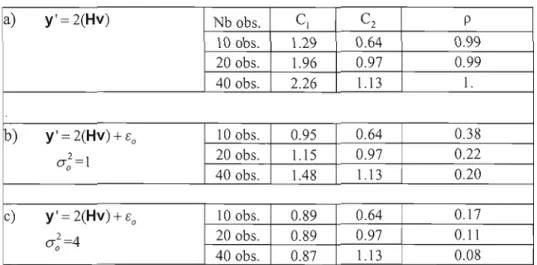
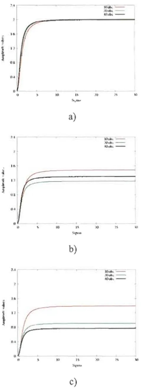
Figure Page 2.1 Variation of the amplitude increment for different values of associated with

the three experiments for which B = (j2 VV T and the observation en'or is a)

0";

=

0, b)

0";

=1, and c)

0";

=4. In each case, experiments were done with

10, 20 and 40 observations . 41

2.2 Analysis increments obtained with an adapted lD-Var (in black), and a standard lD-Var (in red). The sensitivity function used in the analysis is also shown (dotted line). The observations are shown as crosses or dots for the two experiments. In ail cases, the adapted 1D-Var used (j = 10: a) the observations were generated by sampling the sensitivity structure function used in the analysis, b) the observations were generated from a function

con'esponding to a different structure function . 42

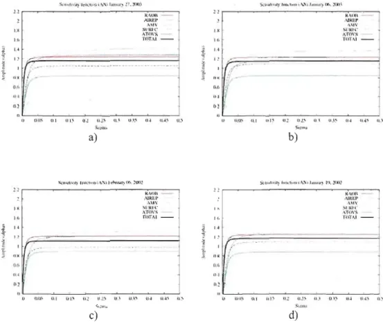
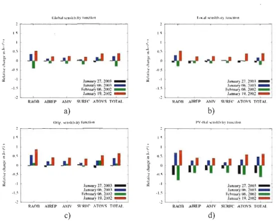
2.3 Amplitude of the analysis increment as a function of parameter (j for different families of observational data: radio soundings (RAOB), aircraft data (AIREP), wind vectors derived from satellite data (AMV), surface and ship data (SURFC), radiance data from satellite (ATOVS) and ail observations combined (TOTAL). The 3D-Var analyses are used as sensitivity function to adapt the background error covariance matrix for 4 case studies: a) January 27, 2003; b) January 06, 2003, c) February 06, 2002,

d) January 19,2002 . 43

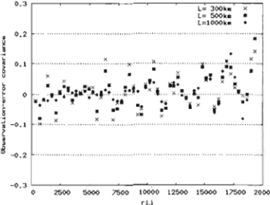
2.4 Relative change in the global fit to the observations for different families of observational data. The a posteriori sensitivity functions are used as structure functions in the adapted 3D-Var for 4 case studies. A positive value means that the adapted 3D-Var analyses are farther away from the observations than the operational analysis and a negative value means that the adapted 3D-Var analyses fit the observations values better than 3D-Var... 44 3.1 Off-diagonal tenns in the observation error covariance as function of

distance r_ij between points i and j. . ₇₀

3.2 The total DFS two-month averaged (January-February 2007) in the MSC 3D- Var and 4D-Var analysis over the four regions: ail globe, over the northem hemisphere (20N-90N), over the tropics (20S-20N) and over the

southem hemisphere (90S-20S) . 71

3.3 DFS two-month averaged (January-February 2007) in the MSC 3D/4D-Var

3.4 Observation influence in the MSC 3D/4D-Var analyses for the eight data

types over globe . 73

3.5 DFS two-month averaged over ail globe in the MSC 3D/4D-Var analyses for

each channel of (a) AM SU-A and (b) AMSU-B . 74

3.6 Degree offreedom for signal for the main data types in the 3D-Var and 4D­ Var data assimilation systems as a function of observation time relative to the assimilation window. The observing platforms are color-coded and given

in the legend .. 75

4.1 Areas (in grey) where (a) profiling observations (radiosonde, aircraft and wind profiler data are denied over North America. (b) The Canadian Arctic, Canada and continental United States regions chosen to examine the impact

of observation on analyses . 102

4.2 North America data denial experiments. Averages values of DFS for eight families of observational data (see text for description) in the control experiment (red bars), in the NO_RAOB (green bars) and NO_AIRCRAFT (blue bars) experiments inside the North America region. Results with 3D­ Var are in the left panel while those wi th 4D-Var are in the l;ght panel. ... 103 4.3 Same as Fig. 4.2 but over: a) Canadian Arctic, c) Canada and e) continental

United States for the experiments with 3D-Var. Results with 4D-Var are in b) Canadian Arctic, d) Canada and f) continental United States. Experiments shown for each region include, from left to right, the control simulation and denials of radiosonde and wind profiler (NO_RAOB) and aircraft data

(NO_AIRCRAFT) over the North America . 104

4.4 North America 4D-Var data denial experiments. Averages values of DFS for eight families of observational data (see text for description) for the experiments CTRL (red bars), NO_RA OB (green bars), NO_AIRCRAFT (blue bars), NO_ASCENT-DESCENT (orange bars) and NO_RAOB_NO_AIRCRAFT (bars) inside a) Canadial1 Arctic, b) Canada

and c) continental United States regions .. 105

4.5 _{Averages values of F'~::;n and DFSregiol1 during January-February 2007} for two observation sets (k=RAOB+PR; AI;) over the different regions (North America, Canadian Arctic, Canada and Continental US). Results with 3D-Var are in the left panel while those with 4D-Var are in the right panel. .. 106 4.6 Forecast impact (%) for 500 hPa geopotential heights of the OSEs

experiments (NO_RAOB, NO_AI) at 12 hours fore cast period over four

Tableau Page 2.1 Coefficients CI and C₂ and correlation coefficient p computed using 1D­

Var assimilation system for three experiments. a) perfect observation, b)

a;

=

l ,c)

a;

=

4.

In

each case, experiments were done with 10,20 and 40

observations . 37

2.2 Correlation coefficient computed for different data types and for ail observations combined. Different sensitivity functions from the key analysis elTor algorithm are used: GLOBAL (initial corrections that minimized the 24-h forecast error over the globe); LOCAL (initial corrections that minimized the 24-h forecast error over an area on the East coast of North America); HEMISPHERIC (initial corrections over the latitudinal band 25N-90N); PV-BAL (balanced initial corrections over the latitudinal band 25N-90N). Cases shown are a) January 27, 2003, b) January 06, 2003, c) February 06, 2002, d) January 19,2002 . 38 2.3 Correlation coefficient computed for different data types and for ail

observations combined. The 3D-Var analyses are used as sensitivity function to adapt the background error covariance matrix for 4 case studies: a) JanualY 27,2003; b) January 06, 2003, c) February 06, 2002, d)

January 19,2002 .. 39

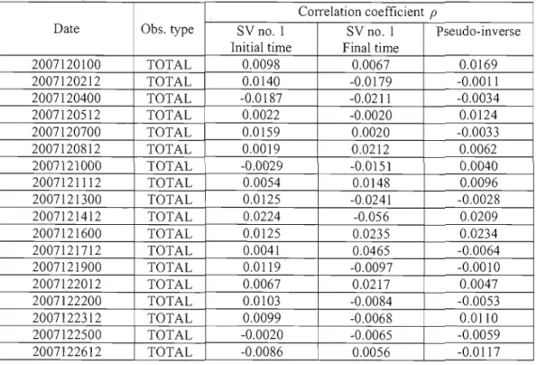
2.4 COITelation coefficient computed for ail data types for 18 cases of December 2007. The first singular vector at initial and final time and the

pseudo-inverse are used as structure function . 40

3.1 DFS estimate values as function of background cOITelation length-scale (Le). DFSAN.-tLYTfC as calculated from the true gain matrix, _DFSCTRARD as computed with Girard's method,

DFS~I~OST' DFS~~OST

and DFSD1ACas obtained from eq. (28)-(30). (The a priori values are perfectly known

(J~ = (J~(t) =

4.,

(J~ = (J~(t) = 1. .. ₇₆

3.2 _{Same as in Table 3.1 but for expeliment with (J~}

₌

_(J~(I)

₌

_1.

_{and an} underestimated value of observation error variance (a~ = 2.25) . ₇₇ 3.3 Same as in Table 3.1 but for the experiment with both the observation and

background error variances underestimated (a~

=

2.25 and (J;

=

0.25

3.4 List of observations assimilated in 3D and 4D-Var assimilation systems of

the Environment Canada during winter 2006-2007 . 79

3.5 _{Comparison between estimated values of chi square X}2

and the number of observation p in 3D-Var and 4D-Var averaged for a two-month winter

period (l January to 28 February 2007) . 80

4.1 Averages values of DFS with 3D-Var and 4D-Var for January, February and during January-February 2007 for three regions (Canadian Arctic,

AIRS AMSU-A/B AMV ATOVS ATReC CMC DFS ECMWF EnKF FASTEX GOES GEM IASI IC MOmS MSC NORPEX NMC NWP OSEs

RAdB

RRKF

Atmospheric Infra-Red Sounder

Advanced Microwave Sounding Unit (A and B) Atmospheric Motion Vectors

Advanced TIROS Operational Vertical Sounder Atlantic THORPEX Regional Campaign Centre Météorologique Canadien Degree of Freedom of Signal

European Centre for Medium range Weather Forecast Ensemble Kalman Filter

Fronts and Atlantic Storm-Track Experiment Geostationary Operational Envirorunental Satellite Global Environnemental Multi-échel1e

Infrared Atmospheric Sounding Interferometer Information Content

MODderate-resolution Imaging Spectroradiometer Meteorological Service of Canada

NoIth Pacifie Experiment National Meteorological Centre Numerical Weather Prediction Observing Systems Experiments Radio soundings Observations Reduced-Rank Kalman Filter

SVs Singular Vectors

SVD Singular Value Decomposition

T-PARC THORPEX Pacific-Asia Regional Campaign

UTC Coordinated universal time

o Degré

0-

1 _{Opérateur inverse}

0°

Opérateur adjoint

cl

Opérateur de transposition (.)0 Indice relatif au moment initial

0

Indice relatif à l'analyse

0

Ob

Indice relatif à l'ébauche

0

Indice relatif aux observations

0

(.,.) Produit scalaire

% Pour cent

V Opérateur gradient d'une fonction

vv

T _{Opérateur hessien d'une fonction}

A Matrice de covariance d'erreurs d'analyse

A Matrice de covariance d'erreurs d'analyse a posteriori B Matrice de covariance d'erreurs d'ébauche du 3D-Var B Matrice de covariance d'erreurs d'ébauche a posteriori

B

Matrice de covariances d' elTeurs d'ébauche du 3D-Var adapté

x

CI Coefficient de projection de l'innovation sur la direction de sensibilité

Écarts de l'analyse à l'ébauche

Différences entre l'analyse et les observations

Différences entre le modèle de prévision et les observations

o

E[.]

f H H J

Matrice de covariance de l'innovation.

Matrice de covaliance de l'innovation a posteriori Espérance mathématique

Vecteur direction de sensibilité (dans l'espace de D'x Opérateur d'observations

Opérateur d'observations linéarisé Matrice identité

Fonction coût

Partie de la fonction coût liée à l'ébauche Partie de la fonction coût liée aux observations

K Matrice de gain

Matrice de gain a posteriori

L Longueur du domaine ID-Var Longueur de corrélation p

R R

s

Nombre total d'observations

Matrice de covaliances d'erreurs d'observations

Matrice de covariances d'erreurs d'observations a posteriori Matrice d'influence

Ir Trace

v

Vecteur direction de sensibi lité normalisé (dans l'espace de ox)

v Vecteur direction de sensibilité normalisé (dans l'espace de Ç)

x

Vecteur de l'état de l'atmosphère

Vecteur d'état de l'atmosphère à l'instant initial Vecteur analyse

Vecteur analyse correspondant aux observations perturbées

Vecteur de l'ébauche

X, Vecteur de l'état vrai de l'atmosphère

x

Matrice non aléatoire

y Vecteur des observations

.

y Vecteur des observations perturbées

y' Vecteur d'innovation

a

Amplitude de l'incrément d'analyse dans la direction sensible

0(.) Opérateur de perturbation

OX

Vecteur d'état incrémentaI Vecteur des erreurs d'analyse Vecteur des elTeurs de l'ébauche

Vecteur des erreurs de mesure instrumentale Vecteur des erreurs d'observations

a

Opérateur de différentiation partielle

Tf CoordOImée verticale Longitude, latitude (rad) p Coefficient de corrélation

Variance d'erreurs de prévision dans la direction de sensibilité Écart type des erreurs de prévision

Écart type des erreurs d'observations Vecteur d'état préconditionné par B

Vecteur d'état préconditionné par B Chi-carré

L'assimilation de données est une composante essentielle du système de prévision numérique du temps et consiste à trouver un état de l'atmosphère, l'analyse, qui est compatible avec les différentes sources d'observations, la dynamique de l'atmosphère et un état antérieur du modèle. Dans ce processus, il est important de bien caractériser l'eneur associée à chaque source d'information (observations, ébauche) afin de mieux décrire les conditions initiales.

La matrice de covariance des elTeurs de prévisions joue un rôle clé dans le processus d'assimilation de données car elle détermine la nature de la correction apportée par l'analyse. Cette matrice étant trop grande pour être représentée explicitement, elle est modélisée sous la fOIme d'une suite d'opérateurs relativement simples. Les modèles de covariance d'eneurs de prévisions utilisées dans un 3D-Var sont généralement stationnaires et ne considèrent pas des variations dues à la nature de l'écoulement. En présence d'instabilité, une petite erreur dans les conditions initiales connaîtra une croissance rapide. Pour contrôler cette croissance d'erreur à courte échéance, il est nécessaire d'apporter des corrections à l'analyse dans des régions localisées selon une stmcture spatiale très particulière. L'assimilation adaptative 3D­ Var considère une formulation différente des covariances d'erreur de prévision qui pennet d'inclure les fonctions de structure basées sur des fonctions de sensibilité a posteriori et a

priori définissant la structure de changements aux conditions initiales qui ont le plus d'impact sur une prévision d'échéance donnée. Dans le cadre de cette thèse, des fonctions de sensibilité sont introduites comme fonctions de structure dans l'assimilation 3D-Var. La définition d'une fonction de structure appropriée pour un système d'assimilation vise à simultanément concorder aux observations disponibles et améliorer la qualité des prévisions. L'observabilité des fonctions de structure par les observations est tout d'abord présentée et analysée dans le cadre plus simple d'une analyse variationnelle 1D (ID-Var) pour être ensuite introduite dans le 3D-Var d'Environnement Canada. L'amplitude de la correction est caractéJisée par un seul paramètre défini par l'ensemble des observations disponibles. Les résultats montrent que si le rapport entre l'amplitude du signal et l'etTeur d'observation est très faible, les observations ne sont pas en mesure de détecter les instabilités atmosphériques qui peuvent croître très rapidement. Dans cette perspective, l'assimilation pourra seulement extraire l'information contenue dans les structures atmosphériques déjà évoluées.

Dans un deuxième temps, nous présentons une nouvelle méthode permettant d'estimer l'impact des observations dans les analyses 3D/4D-Var basé sur le Degrees offreedomfor signal. Le contenu en informations des observations est calculé en employant les statistiques a posteriori, à partir des écarts des observations à l'ébauche et à l'analyse. Les résultats montrent que le DFS estimé en utilisant les statistiques a posteriori est identique avec celui obtenu à partir des statistiques a priori. Ce diagnostic permet de comparer l'importance de différents types d'observations pour les expériences d'assimilation 3D et 4D-Var incluant toutes les observations assimilées opérationnellement. En particulier, cette étude s'intéresse à l'évaluation du réseau canadien d'observations et il est appliqué aux Observing System Experiments (OSEs) effectués à Environnement Canada pour les mois de janvier et février

2007.

INTRODUCTION

L'assimilation de données consiste à trouver un état de l'atmosphère, l'analyse, qui soit compatible avec les différentes sources d'observations, la dynamique de l'atmosphère et un état antérieur du modèle. Dans le processus d'assimilation de données, il est fondamental de bien caractériser l'erreur associée à chaque source d'information (ébauche, observations) afin de mieux caractériser les éléments du système d'analyse qui peuvent influencer la qualité des prévisions. Étant donné que l'état vrai de l'atmosphère n'est pas accessible, il est impossible d'obtenir directement des échantillons des erreurs d'ébauche et d'observation et ces erreurs doivent donc être estimées a priori à partir de statistiques. L'étude des innovations d'un jeu d'observations suffisamment grand et dense fournit des statistiques permettant de construire les matrices de covaliance d'elTeurs (Hollingsworth et Lonnberg, 1986). Toutefois, 1'hypothèse que les erreurs d'observation ne sont pas cOITélées spatialement est fondamentale car seule cette hypothèse pennet de séparer l'information provenant de la matrice de covariances d'erreur d'observation R et d'ébauche B.

D'autres méthodes permettent d'estimer les covariances d'erreur d'ébauche, par exemple la méthode du National Meteorological Centre (NMC) (Parrish et Derber, 1992). Cette méthode consiste à estimer les covariances d'erreur de prévision à partir des différences entre deux prévisions valides au même moment, mais à des échéances différentes.

À

Environne­ ment Canada, les différences entre les prévisions à une échéance de 48-h et à 24-h respective­ ment sur une période de deux ou ti'ois mois sont employées (Gauthier et al., 1998).

Dans le 3D-Var, des hypothèses telles que la stationnarité, l'homogénéité et l'isotropie sont souvent imposées pour simplifier la modélisation des covariances d'erreur de prévision. Les systèmes d'assimilation de données doivent être capables de représenter, par exemple, les structures baroclines pour être en mesure de décrire correctement les phénomènes pour lesquels une petite erreur d'analyse conduit à des erreurs majeures de prévision. Dans ce

cadre, des recherches ont été réalisées pour améliorer l'estimation et la représentation des covariances d'erreurs de prévision et prendre en compte les variations dues à la nature de l'écoulement dans la matrice de covariance d'erreur de prévision.

Des études de sensibilités a posteriori (Rabier et al., 1996; Klinker et al., 1998) et a priori (Hello et a!., 2000) basées sur l'utilisation du modèle adjoint (Le Dimet et Talagrand, 1986) ont été développées afin de contrôler les erreurs sur les conditions initiales susceptibles de croître rapidement. Les fonctions de sensibilité a posteriori permettent de caractériser des cOlTections aux conditions initiales qui peuvent réduire significativement l'erreur de prévision à une échéance donnée (typiquement 24 ou 48 heures). L'erreur de prévision est définie par l'écart à une analyse de vérification et la fonction de sensibilité ne peut donc être calculée qu'a posteriori. Les fonctions de sensibilité a priori sont utilisées pour réduire la pa11 des erreurs de prévision due aux conditions initiales sans attendre l'analyse de vérification. Pour évaluer la sensibilité d'une prévision aux changements aux conditions initiales, la fonction de sensibilité a priori est définie par rapport à un aspect particulier de la prévision à un temps ultérieur et on détermine ensuite la correction aux conditions initiales qui a le plus d'influence sur cet aspect particulier de la prévision. Cette idée peut être généralisée et l'emploi du modèle adjoint permet aussi le calcul des vecteurs singuliers qui représentent le sous-espace dans lequel des changements aux conditions initiales subissent le plus d'amplification sur une période donnée. Les vecteurs singuliers et les études de sensibilité aux conditions initiales permettent d'identifier pour chaque situation météorologique, les régions sensibles, où la moindre eneur sur les conditions initiales peut croître très rapidement et avoir un effet considérable sur la qualité de la prévision. Dans ces régions, il semblait naturel d'ajouter de nouvelles observations (observations ciblées) afin d'augmenter la précision de l'analyse et réduire de manière notable l'erreur de prévision. La technique de l'observation adaptative a été testée lors de différentes campagnes de mesures avec ciblage des observations: Fronts and Atlantic Storm- Track Experiment (FASTEX, Joly et a!., 1999), North Pacific Experiment (NORPEX, Langland et aL., 1999),2003 Atlantic THORPEX Regional Campaign (ATReC, Langland, 2005) et tout récemment 2008 THORPEX Pacific-Asia Regional Campaign (T-PARC). Les résultats de ces expériences ont montré que l'impact de données ciblées n'est perçu que si de grandes régions sont échantillonnées et les systèmes d'assimilation variationnelle de données 3D-Var et même le

4D-Var ne peuvent extraire toute l'infonnation apportée par ces données ciblées. La valeur des campagnes de ciblage des observations doit être reconsidérée dans le contexte où le déploiement des observations ciblées n'a qu'un impact faible mais néanmoins significatif sur la réduction des erreurs de prévision. Toutefois, l'infonnation contenue dans les sensibilités devrait être considérée pour le déploiement des observations.

Hello et Bouttier (2001) ont introduit localement dans le 3D-Var les fonctions de sensibi­ lité a priori comme fonction de structure. Leur méthode consistait à représenter les covarian­ ces d'errem pour une sous-partie de la matrice B en suivant la procédure développée pour le filtre de Kalman de rang réduit (RRKF) par Fisher (1998). Essentiellement, cette approche traite différemment la partie de la variable de contrôle qui se projette dans l'espace décrivant la composante sensible. Ceci rejoint la fonnulation de modèles de covariance d'erreur de prévision basés sur les vecteurs singuliers (Fisher et Andersson, 2001; Buehner, 2004). Présentement, des approches hybrides considèrent dans l'assimilation variationnelle 4D-Var des modèles de covariance d'erreurs de prévision dépendant de l'écoulement obtenus par des méthodes d'ensembles (Buehner et al., 2010 a,b; Berre et al., 2009)

Au cours des dernières années, d'importants changements ont été introduits dans les systèmes d'assimilation de données des centres opérationnels de prévision numérique du temps afin de permettre une meilleure utilisation des données provenant d'un nombre croissant d'instruments embarqués sur satellites. Actuellement, les données satellitaires constituent la plus importante source de données utilisée pour l'analyse météorologique en vue de la prévision numérique du temps. Par exemple, à l'ECMWF les radiances satellitaires représentent 90% du nombre total d'observations assimilées. Le monitoring et le contrôle de données sont abordés par le contrôle systématique des écarts entre le modèle de prévision et les observations et entre l'analyse et les observations.

Les elTeurs d'observation sont souvent censées être non corrélées et la matrice de covariance d'en"eurs d'observations R est alors diagonale dans les schémas d'assimilation opérationnels. Si cette hypothèse paraît raisonnable pour des observations mesurées par des instruments différents, elle est moins évidente quand un jeu d'observations est obtenu par le même instrument de mesure ou quand une série temporelle de mesures d'une même station est utilisée dans un 4D-Var (Jarvinen et al., 1999). L'elTeur d'observation renferme l'erreur

de mesure instrumentale, l'erreur due aux imperfections dans le modèle de transfel1 radiatif et les erreurs de représentativité. La variabilité sous maille de la variable observée, qui n'est pas résolue par le modèle, mais qui peut être mesurée par l'instrument, est à l'origine de l'erreur de représentativité. Dans le cas d'observations satellitaires, l'erreur d'observation est corrélée spatialement, temporellement, et spectralement puisqu'elles sont prises avec le même instrument et dans les mêmes conditions. Liu et Rabier (2002) ont montré que l'omission des corrélations d'erreur d'observation dans la matrice R pOUiTait être compensée par une augmentation des valeurs de l'écart type d'elTeur d'observation ou encore en réduisant le volume de données.

L'estimation des erreurs d'observations peut être faite à partir de comparaisons entre les observations ou avec la méthode basée sur les innovations (Hollingsworth et Lormberg, 1986). Plus récemment, Desroziers et al. (2005) ont développé des nouvelJes approches qui permettent d'estimer la matrice de covariance d'erreur d'observations et la matrice de cova­ riance d'erreur d'ébauche dans l'espace des observations à partir des écarts des observations à l'ébauche et à l'analyse.

L'estimation de l'impact des observations dans l'analyse et dans les prévisions à courte échéance est un enjeu important dans les centres de prévision numérique du temps. Différentes méthodes ont été développées et examinées dernièrement afin de quantifier le contenu en information des observations dans les analyses et dans les prévisions à courte échéance. Le Degrees of freedom for signal (ou DFS) est un diagnostique pelmettant d'évaluer le contenu en information apportée par les différents types d'observations dans l'analyse (Rodgers, 2000). En particulier, les observations issues de sondeurs infrarouges hyperspectraux dont les premiers embarqués sont AIRS (Atmospheric lnfrared Sounder) et IASI (Infrared Atmospheric Sounding Interferometer) apportent un précieux contenu en information sur l'état de l'atmosphère mais comprerment une grande quantité des données. Un enjeu important est donc de mettre en place de méthodes de sélection de données permettant de faire un bon compromis entre le volume de données, la qualité de l'analyse et l'impact sur les prévisions. Un exemple de la façon dont le DFS a été appliqué pour la sélection de canaux de dormées simulées IASI est présenté dans Rabier et al. (2002). À ECMWF, Cardinali et al. (2004) ont utilisé la matrice d'influence pour évaluer la sensibilité

de l'analyse 4D-Var aux observations. Le contenu en information pour les différentes familles d'observations dans des régions géographiques diverses est estimé à partir des éléments diagonaux de la matrice d'influence. Fisher (2003) a examiné la possibilité d'évaluer le

DFS

exprimé conune la trace de la matrice d'influence pour le 4D-Var de l'ECMWF. La méthode de Girard (1987) permet également d'exprimer la trace d'une matrice très large par une procédure de randomisation. Une telle procédure a été également employée par Chapnik et al. (2006) à Météo-France.

L'impact des observations sur l'erreur de prévision à courte échéance est évalué avec la méthode de calcul de sensibilité aux observations (Baker et Daley, 2000; Doerenbecher et Bergot, 2001; Langland et Baker, 2004; Zhu et Gelaro, 2008; Cardinali, 2009). D'autre part, les Observing System Experiments (OSEs) sont également utilisées dans les centres de prévision numérique du temps pour diagnostiquer l'impact des observations dans un système de prévision. Ceci est obtenu à partir des OSEs dans lesquels certains types de données sont systématiquement ajoutés ou retirés du système d'assimilation (Kelly et al., 2007). Il est à noter que l'impact de chaque type d'observation dépend de la méthode d'assimilation de données, du modèle de prévision et des erreurs des observations et de l'ébauche considérée dans le processus d'assimilation.

Le travail effectué dans cette thèse est présenté en cinq chapitres dont trois correspondent à des articles écrits en anglais qui seront soumis pour publication. Le présent chapitre introduit la problématique et le contexte général de la recherche et résume les objectifs et le plan de l'étude.

Le deuxième chapitre est constitué d'un article intitulé « Observability offlow dependent structure functions for use in data assimilation» par Cristina Lupu et Pierre Gauthier, et il sera soumis pour publication dans Monthly Weather Review. Tout d'abord, le système d'assimilation de données doit être capable de prendre en compte les structures baroclines pour être en mesure de décrire correctement les phénomènes pour lesquels une petite erreur d'analyse conduit à des erreurs majeures de prévision. Hello et Bouttier (2001) ont proposé ce qu'il est convenu d'appeler le 3D-Var adapté, basé sur une formulation différente des covariances d'erreur de prévision qui permet d'inclure l'information sur les instabilités atmosphériques contenue dans une fonction de sensibilité. Une variante du 3D-Var adapté a

été introduite par Lupu (2006) et considère que le modèle de covariance d'erreur de prévision du 3D-Var adapté inclut la composante sensible tout en retenant le modèle plus conventionnel du 3D-Var lorsque cette composante dite sensible est peu importante. En conséquence, le premier point vise à examiner des formulations différentes des covariances d'erreur de prévision, qui permettraient d'inclure à même le processus d'assimilation l'information sur les instabilités atmosphériques contenue dans une fonction de sensibilité. A ce titre, il faut réaliser que la caractérisation de ces structures instables dépend du modèle utilisé pour les générer et de la façon dont on définit la mesure de l'erreur de prévision. Dans un premier temps, nous présentons brièvement l'algorithme 3D-Var et sa version 3D-Var adapté proposé et validé par Lupu (2006). Dans un deuxième temps, le problème d'assimilation est formulé dans le sous-espace engendré par la fonction de sensibilité. Ceci nous conduira à la question d'observabilité des fonctions de structure qui sera formulée et discutée dans un contexte 1D-Var avec quelques exemples simples. Étant donné que les fonctions de sensibilité a posteriori définissent les changements aux conditions initiales qui réduisent significativement l'erreur de prévision à une échéance donnée, il parait logique de les inclure dans la matrice de covariance d'erreur de prévision du 3D-Var. Dans ce cas, l'amplitude de cette correction est déterminée en s'ajustant aux observations disponibles. Nous présentons différentes définitions des fonctions sensibles a posteriori qui seront introduites comme fonctions de structure dans le modèle de covariance du 3D-Var. Nous allons examiner si le 3D-Var adapté permet d'améliorer l'ajustement de l'analyse aux observations tout en ayant un impact sur la qualité de la prévision comparable à ce qui est obtenu avec les analyses de sensibilité a posteriori, Enfin, pour valider la méthode, l'incrément de l'analyse du 3D-Var normalisé est introduit comme fonction de structure dans le modèle de covariance du 3D-Var qui inclut cette seule composante sensible. Ceci a permis de vérifier dans ce cas que les observations permettent d'estimer cOlTectement l'amplitude de l'incrément du 3D-Var. Par contre, tel n'est pas le cas si on utilise les analyses a posteriori. Ceci nous a conduit à définir la notion d'observabilité d'une fonction sensible qui pennet d'établir si les observations sont en mesure de détecter une telle structure.

Les bases du troisième chapitre sont nées des questions qui ont émergé des études d'impact des observations dans les analyses et dans les prévisions. Ce chapitre est constitué d'un article intitulé « Evaluation of the impact of observations on analyses in 3D and 4D- Var

based on information content» par Cristina Lupu, Pierre Gauthier et Stéphane Laroche, et il sera soumis pour publication dans Monthly Weather Review. Dans ce chapitre, nous nous intéressons à évaluer l'impact des observations dans les analyses 3D and 4D-Var (Gauthier et al., 1999, 2007). Nous proposons une nouvelle méthode qui permet l'estimation du

DFS

à partir des écarts des observations à l'ébauche et à l'analyse. Cette méthode sera illustrée et validée dans le cadre plus simple d'une analyse variationnelle ID (lD-Var) et ensuite appliquée pour évaluer le contenu en informations des observations assimilées avec le 3D et 4D-Var.

Dans la suite de cette étude, le quatrième chapitre se concentre sur l'évaluation du

DFS

pour différentes familles d'observations à l'aide d'OSE (Observing System Experiments). II est constitué d'un article intitulé

«

Assessment of the impact of observations on analyses derived/rom observing systems experiments

»

par Cristina Lupu, Pierre Gauthier et Stéphane Laroche, et il sera soumis pour publication dans Monthly Weather Review. Après une brève description des expériences OSEs réalisées par Laroche et Sarazzin (20 l 0 a, b), nous allons mesurer l'impact des différents types de données dans les analyses 3D et 4D-Var en évaluant le contenu en information des observations sur différentes régions sur AméJique du Nord. Cette étude est complémentaire à celle de Laroche et Sarazzin (2010 a, b) qui ont réalisé les OSEs ayant servi de base à notre étude.

Le chapitre V résumera les principaux résultats obtenus dans ces études et quelques perspectives de recherche ouvertes par ce travail seront proposées.

Baker N. L. and R. Daley, 2000: Observation and background adjoint sensitivity in the adaptative observation-targeting problem. Q. 1. R. Meteorol. Soc., 126, 1431-1454. Berre, L., G. Desroziers, L. Raynaud, R. Montroty and F. Gibier, 2009: Consistent

operational ensemble variational assimilation, Procedings of the CA WCR Workshop on Ensemble Prediction and Data Assimilation, Melboume, Australia.

Buehner, M., 2004: Ensemb1e~derived stationary and flow-dependent background error covariances: Evaluation in a quasi-operational NWP setting. Q. 1. R. Meteorol. Soc., 128, 1-31.

_ _ _, P. L. Houtekamer, C. Charette, H. L. Mitchell and B. He, 2010a: Intercomparaison of variational data assimilation and Ensemble Kalman filter for global deterministic NWP. Part I: Description and single observation expeliments, Mon. Weather

Re~138,

1550-1566.

_ _ _, P. L. Houtekamer, C. Charette, H. L. Mitchell and B. He, 201 Ob: Intercomparaison of variational data assimilation and Ensemble Kalman filter for global detem1inistic NWP. Part II: One-month experiments with real observations, Mon. Weather Rev, 138,1567-1586.

Cardinali

c.,

S. Pezzulli and E. Andersson, 2004: Influence-matrix diagnostic of a data assimilation system.

Q.

1. R. Meteorol. Soc., 130, 2767-2786.

- - , 2009: Monitoring the observation impact on the shOlt-range forecast. Q. 1. R. Meteorol. Soc., 135, 239-250.

Chapnik B., G. Desroziers, F. Rabier and O. Talagrand, 2006: Diagnosis and tuning of observational error in a quasi-operational data assimilation setting.

Q.

1. R. Meteorol. Soc., 132, 543-565.

Desroziers G., L. Berre, B. Chapnik and P. Poli, 2005: Diagnosis of observation, background and analysis-error statistics in observation space. Q.1. R. Meteorol. Soc., 131,3385­ 3396.

Doerenbecher, A. and T. Bergot, 2001: Sensitivity to observations applied to FASTEX cases. Nonlinear Pro cesses in Geophysics, 8 (6),467-481.

Fisher, M., 1998: Development of a simplified Kalman Filter. ECMWF Research Dept. Technical Memorandum, no. 260, 16 pp.

_ _ _, and E. Andersson, 2001: Developments in 4D-Var and Kalman filtering. ECMWF Research Dept. Technical Memorandum, no. 347.

_ _ _, 2003: Estimation of entropy reduction and degrees of freedom for signal for large variation al analysis systems. Tech. Rep., 397, ECMWF, 20pp.

Gauthier, P., M. Buehner and 1. Fillion, 1998: Background-error statistics modelling in a 3D variational data assimilation scheme. Proceedings of the ECMWF workshop on diagnosis ofdata assimilation systems, Reading, UK, 131-145.

- - , M. Tanguay, S. Laroche, S. Pellerin, and J. Momeau, 2007: Extension of 3DVAR to 4DVAR: Implementation of 4DVAR at the Meteorological Service of Canada. Mon. Weather Rev., 135, 2339-2354.

Girard, D., 1987: A fast Monte Carlo cross-validation procedure for large least squares problems with noisy data. Tech. Rep. 687-M, IMAG, Grenoble, France, 22pp. Hello, G., F. Lalaurette and J.-N. Thépaut, 2000: Combined use of sensitivity information

and observations to improve meteorological forecasts: A feasibility study applied to the' Christmas storm' case. Q. 1. R. Meteorol. Soc., 126, 621-647.

and F. Bouttier, 2001: Using adjoint sensitivity as a local stmcture function in variationaI data assimilation. Nonlinear Pro cesses in Geophysics, 8, 347-355. Hollingsworth, A. and P. Lonnberg, 1986: The statistical stmcture of short-range forecast

errors as determined from radiosonde data. Part 1: The wind field. Tellus, 38A, 111­ 136.

Joly, A., K. A. Browning, P. Bessemoulin, 1. P. Cammas, G. Caniaux, J. P. Chalon, S. A. Clough, R. Dirks, K. A. Emanuel, 1. Eymard, F. Lalaurette, R. Gall, T. D. Hewson, P. H. Hildebrand, D. Jorgensen, R. H. Langland, Y. Lemaître, P. Mascart, 1. A. Moore, P. O. G. Persson, F. Roux, M. A. Shapiro, C. Snyder, Z. Toth and R. M. Wakimoto, 1999: Overview of the field phase of the Fronts and Atlantic StOlm Track Experiment (FASTEX) project. Q. 1. R. Meteorol. Soc., 125, 3131-3164.

Jarvinen, H., E. Andersson and F. Bouttier, 1999: Variational assimilation of time sequences of surface observations with serially cOlTelated errors. Tellus, 51A, 468-487.

Kelly, G., J. N. Thépaut, R. Buizza and C. Cardinali, 2007: The value of observations. 1: Data denial experiments for the Atlantic and the Pacific. Q. 1. R. Meteorol. Soc., 133,

1803-1815.

Klinker, E., F. Rabier and R. Gelaro, 1998: Estimation of key analysis errors using the adjoint technique. Q. 1. R. Meteorol. Soc., 124,1909-1933.

Langland R. H., Z. Toth, R. Gelaro, 1. Szynyogh, M. A. Shapiro, S. 1. Majumdar, R. Morss, G. D. Rohaly, C. Velden, N. Bonds and C. H. Bishop, 1999: The North Pacific

Experiment (Norpex-98): Targeted observations for improved North American Weather Forecasts. Bull. Am. Meteorol. Soc., 80, 1363-1384.

- - and N. L. Baker, 2004: Estimation of observation impact using the NRL atmospheric variational data assimilation adjoint system. Tellus, 56A, 189-201.

- - , 2005: Observation impact dUling the North-Atlantic TreC-2003. Mon. Weather Rev., 133, 2297-2309.

Laroche, S. and R. SaITazin, 201 Oa: Impact study with observations assimilated over North America and the NOlih Pacifie Ocean on the MSC global forecast system. Pmi I: contribution of radiosonde, aircraft and satellite data. Atmos.-Ocean, 48, 10-25. and R. SalTazin, 201 Ob: Impact study with observations assimilated over North

America and the North Pacifie Ocean on the MSC global forecast system. Part II: Sensitivity experiments. Atmos.-Ocean, 48, 26-38.

Le Dimet F.-X., and O. Talagrand, 1986: Variational algorithms for analysis and assimilation ofmeteorological observations: Theoretical aspects. Tellus, 38A, 97-110.

Liu, Z. Q. and F. Rabier, 2002: The interaction between model resolution, observation resolution and observation density in data assimilation: A one-dimensional study. Q. 1. R. Meteorol. Soc, 128, 1367-1386.

Lupu, C., 2006: Impact d'un modèle de covariance d'erreur de prevIsIon basé sur les fonctions de sensibilité dans un 3D-Var. Mémoire de maîtrise en sciences de l'atmosphère, UQAM, 138 pp.

Parrish, D. F. and 1. C. Derber, 1992: The National Meteorological Center's spectral statistical interpolation analysis system. Mon. Weather Rev., 120, 1747-1763

Rabier, F., E. Klinker, P. Courtier and A. Hollingsworth, 1996: Sensitivity offorecast errors to initial conditions. Q. 1. R. Meteorol. Soc., 122,121-150.

_ _ _, N. Fourrié, D. Chafai and P. Prunet, 2002: Channel selection methods for Infrared Atmospheric Sounding Interferometer radiances. Q. 1. R. Meteor. Soc., 128, 1011­ 1027.

Rodgers,

c.,

2000: Inverse Methods for Atrnospheric Sounding Theory and Practice. World Scientific Publishing, London, 256 pp.

Zhu Y. and R. Gelaro 2008: Observation sensitivity calculations using the adjoint of the Gridpoint Statistical Interpolation (GSI) analysis system. Mon. Weather Rev. 136, 335-351.

ÛBSERVABILITÉ DES FONCTIONS DE STRUCTURE DÉPENDANTES DE L'ÉCOULEMENT POUR UTILISATION EN ASSIMILATION DE DONNÉES

Ce chapitre, rédigé en anglais, est présenté sous la forme d'un article qui sera soumis pour publication dans la revue Monthly Weather Review.

L'assimilation de données joue un rôle important dans l'analyse des données atmosphériques, en paI1iculier pour la prévision numérique du temps. Ce chapitre touche un aspect important de la méthodologie d'assimilation de données qui vise à corriger un état de référence en s'ajustant aux observations en tenant compte d'éléments dynamiques qui pelmettent le développement de systèmes météorologiques. Conséquemment, il est important d'une part de bien caractéJiser les stmctures atmosphériques qui peuvent conduire à une croissance de \' erreur de prévision et d'autre part d'incorporer cette infonnation comme fonction de structure dans le système d'assimilation de données. La question d'observabilité des fonctions de structure sera tout d'abord fonnulée et discutée dans un contexte ID-Var avec quelques exemples simples, pour être ensuite discutée dans le cadre du 3D-Var d'Environnement Canada.

ÛBSERVABILITY OF FLOW DEPENDENT STRUCTURE FUNCTIONS FOR USE IN DATA ASSIMILATION

by

Cristina Lupu',l and Pierre Gauthier]

Department ofEarth and Atmospheric Sciences Université du Québec à Montréal (UQAM)

Montréal (Québec), CANADA

Submitted to Monthly Weather Review

16 March 2010

Corresponding author: Department ofEarth and Atmospheric Sciences Université du Québec à Montréal (UQAM) P.O. Box 8888, Suce. Centre-ville

Montréal, Québec CANADA H3C 3P8

Abstract

One of the objectives of data assimilation is to produce initial conditions that will improve the quality of forecasts. Studies on singular vectors and sensitivity studies have shown that small changes to the initial conditions can sometimes lead to exponential error growth. This has motivated research to include flow-dependent structures within the assimilation that would have the characteristics to correctly predict the growth or decay of meteorological systems. This relates to the characterization of precursors to atmospheric instability. In this paper, the observability of such structures by observations is discussed. Several studies have shown that deploying observations over regions where changes in the initial conditions may impact the forecast the most do not lead to the expected benefit. In this paper, it is shown that given the small magnitude of the signal to be detected, it is important to take into account the accuracy of the observations. If the signal-to-noise ratio is too low, observations cannot detect and characterize precursors to forecast error growths. From that perspective, the assimilation only has the possibility to extract information about evolved structures of error growth. Experiments with a simple ID-Var system are presented and then, with an adapted 3D-Var system with different sensitivity structure functions is used. The results have been obtained by adapting the variational assimilation system of Environment Canada.

2.1 INTRODUCTION

The accuracy of analyses produced by data assimilation systems depends on the precision of background and observation error covariances specified as input. The modelling and estimation of these covariances is critical for any data assimilation system in the context of numerical weather prediction (NWP). Aigorithms like the three-dimensional variational data assimilation (3D-Var) produce analyses by blending together observations neal' the analysis time with a background state provided by a short-term numerical weather prediction. In this case, the background-error statistics are taken to be stationary and do not reflect the flow­ dependency of error growth that depends on the particular meteorological situation. Flow­ dependent covariances can be obtained from approximate forms of the Kalman filter like the ensemble Kalman filter (Evensen, 1994; Houtekamer and Mitchell, 2009).

Instabilities in atmospheric flows can be triggered by small perturbations to initial conditions and these can be characterized using adjoint methods that enable to trace back the source of errors in a forecast to errors in the analysis. Lacan'a and Talagrand (1988) showed that it is possible to characterize the structure of perturbations to the initial conditions that would lead to the most significant growth over a finite period of time. Those correspond to the so-called singular vectors that define the unstable subspace containing those pelturbations that will expelience the most significant error growth. This has been the foundation of the design of ensemble prediction systems that aim to determine how errors in the analysis and the model will lead to forecast errors in the medium -range (Molteni et al., 1996; Buizza et al., 2007).

Since it is possible ta characterize those regions where perturbations in the analysis can lead to important error growth, the next logical step was to use this information to deploy observations in those areas where a reduction in the analysis error could lead to the most important reduction of the forecast error. This is the basis of targeting methods, which use information from singular vector or sensitivitygradients to plan the deployment of adaptive observations. The FASTEX campaign (Joly et al., 1999) was the first to test targeting methods and observations were deployed according to sensitivity gradients, that correspond

to a single singular vector. Other campaigns followed like NORPEX (Langland et al., 1999),

the 2003 Atlantic THORPEX Regional Campaign (ATReC) (Petersen and Thorpe, 2007; Langland, 2005) and recently, the 2008 THORPEX Pacific-Asia Regional Campaign (T­ PARC). From ail those campaigns, the conclusions are that the impact of observations deployed over sensitive areas in the extra-Tropics identified from singular vectors .is, on average, about twice that of any other single observation, but the overall impact is small because of the large volume of data now assimilated (Langland, 2006; Kelly et al., 2008; Buizza et al., 2008; Cardinali et al., 2008). These results bring us to reconsider the value of expensive observation campaigns for the sole purpose of assessing if targeted observations do lead to significant reduction of the forecast eITOr. The current wisdom is that, if observations are to be deployed, it is tl1en appropriate to take into account sensitivity information to do it. Particularly, this may be valuable for adaptive data selection for satellite data. Currently, due to limitations in the assimilation systems, a small fraction of the incoming volume of satellite data can be assimilated (Liu and Rabier, 2001). Adaptive data selection is now being considered to assess whether this results in improvements in the quality of forecasts.

Fisher and Andersson (2001) have proposed a reduced -rank Kalman filter (RRKF) that restricts the evolution of the forecast error covariances within an unstable subspace spanned by singular vectors. Their experimentation was thorough and went aIl the way to include the RRKF to provide the background error covariances for the ECMWF 4D-Var assimilation. This was found to lead to a positive but small impact on the resulting forecasts, which was not deemed significant enough to imp1ement this approach in the ECMWF operational suite. Currently, hybrid approaches have been proposed in which ensemble methods are used to define a subspace that is appropriate to describe the evolved background error covariances (Buehner et al., 201 Oa;b; Ben'e et al., 2009). The preliminary results are very positive and this has sparked a renewed interest to include flow dependent background error covariances when cycling a 4D- Var assimilation system.

This paper has the objective to investigate sorne issues associated with the use of sensitivity information in the representation of background error covaliances with a 3D-Var assimilation system. Hello and Bouttier (2001) did propose an approach through which a priori sensitivity infOimation from a single singular vector was included within the

background error covaIiance matrix, denoted by B. Their approach is called an adapted 3D­ Var as it includes sorne flow dependency. The a priori sensitivity was used to deploy targeted data during the FASTEX campaign (Hello et al., 2000). In the present paper, a variant of their algorithm is presented and tested both in a simple ID-Var context and in 3D-Var. The rationale on which this study is based is the following.

The 24 or 48-hr forecast elTor can be evaluated by comparing with respect to a verifying analysis and the adjoint of the forecast model can be used to define the change in initial conditions that would reduce the forecast elTor. This is referred to as key analysis errors, a telm coined by Klinker et al. (1998) and has been the object of several studies afterwards, (Laroche et al., 2002; Langland et al., 2002; Caron et al., 2007a). This will be refelTed to as an a posteriori sensitivity function because it can only be obtained as a diagnostic of the origin of forecast error. In addition, a priori structure functions defined either as leading singular vectors (SVs) or from the gradient sensitivity vector method (Hello et al., 2000) are tools that have been widely applied in sensitivity studies, particularly for the development of targeting techniques. In the gradient sensitivity vector method, the cost function can be defined with respect to a particular aspect of the forecast at a later time and then find out what are the changes to the initial conditions that will impact the most the forecast error growth. For example, taking the average of sUlface pressure of a 24-h forecast over an area of interest, one can then identify areas where changes in the CUITent analysis could have a significant impact as defined by the sensitivity cost function. In Hello et al. (2000), this has been used to identify those regions where small changes to the initial conditions can be expected to lead to substantial changes in the forecast.

If a posteriori key analyses, as proposed by Klinker et al. (1998), do result in a dramatic reduction of forecast enor, it would make sense to use those as structure functions within the B matrix so that observations would be used to define its amplitude. What was expected is that the amplitude of the key analysis would be recovered. However, this is not what happened. On second thought, the signal that was to be recovered being very small, this raised the question whether those structures could be detected at ail by the observations, which contain sorne amount of observation error.

The paper is organized as follows. Section 2.2 briefly presents the formulation of the variational 3D-Var data assimilation system and its adapted 3D-Var version. Section 2.3 presents the assimilation in the subspace spanned by a single sensitive direction. A particular point concems the observability of a structure function defined from a posteriori sensitivity. Results with a simple ID-Var model are presented in section 2.4 to illustrate the new approach. Section 2.5 introduces different a posteriori sensitivity structures chosen for this work and results based on adapted 3D-Var experiments are described in section 2.5. Finally, section 2.6 summarizes the results and presents sorne conclusions.

2.2 FLOW-DEPENDENT STRUCTURE FUNCTIONS IN 3D-VAR: THE ADAPTED 3D­

VAR

When representing the background error covanance matrix B in a subspace of low dimension with respect to that of the control variable, a regularization term can be added based on the usual 3D-Var covariances with homogenous and isotropie correlations. This can be done in different ways (Fisher, 1998; Hamill and Snyder, 2000). Here, a variant of the method of Hello and Bouttier (2001) is proposed.

2.2.1 3D variational assimilation

The three-dimensional variational (3D-Var) data assimilation used here has been developed at Environment Canada and is described in Gauthier et al. (1999,2007). The basic objective of 3D-Var is to obtain the best estimate of the true atmospheric state at the analysis time. In its incremental form, the analysis increment is ox = x - xb where x is the model state and

X_{b ,} the background state and ox is obtained by minimizing the cost function

where Band R represent the background and observation error covariance matrices respective!y, y'=y-H(x_{b )} is the innovation vector, y the observation vector and H is the linealized version of the observation operator H that maps the model state vector X to observation space. For sake of simplicity, it is assumed that there are no outer iterations. At

its minimum, (1) yields the analysis increment

oX

_a that is added to the background to ob tain the analysis x_a defined as

X _a =x_b +ox_a =x_b +Ky' (2)

where K stands for the Kalman gain matrix expressed as

(3) In 3D-Var, the background error covariances are represented as a stationary matrix. Recently, the assimilation system of Environment Canada has been extended to 4D-Var (Gauthier el al. 2007), in which the background state is compared to the observations at the exact observation time. Moreover in 4D-Var, the background error statistics are implicitly evolved over the assimilation window, which makes them flow-dependent. This slightly relaxes the assumption of stationarity implicit in 3D-Var. In the context of the cycling process of any data assimilation system, it may be impOltant to include a flow-dependent [orm for the background-error covariances to account for the evolved covariances from the previous assimilation (Fisher and Andersson, 2001; Buehner, 201 Oa,b).

2.2.2 Adapted 3D-Var approach

1'0 account for anisotropie atmospheric flow, flow dependence can be included in B. The approach at ECMWF has been to explicitly incorporate, within the background-elTor covariance matrix of 4D-Var, a flow-dependent component defined in a subspace spanned by the leading Hessian singular vectors. This is referred to as a reduced-rank Kalman filter (RRKF) (Fisher, 1998; Beck and Ehrendorfer, 2004). Results demonstrate that the impact of the RRKF is small when the number of Hessian singular vectors used is small compared to the dimension of phase space (Fisher and Andersson, 2001).

In the context of 3D-Var, Hello and Bouttier (2001) proposed to estimate the flow­ dependent background-elTor covariances along a single sensitive direction. This approach uses the adjoint-based sensitivities to define the background-error covariance matrix along that component and the stationary background covariances for the remaining orthogonal subspace. As the spatial structure of the analysis increments is driven by the fOlmulation of

the background error covariance, the result is that the analysis increment gives a representation of the sensitivity structure function and its amplitude is determined from the fit to the observations that project in that direction. Otherwise, the analysis increment gives a representation of the stationary background-euor covariance mattix commonly used in 3D­ Var.

A variant of this approach is proposed here to make corrections to the background along a single sensitive direction. This approach will be referred to as the adapted 3D-Var, for which the background-error covariance model embeds the structure functions as defined by sensitivity functions. The new background-error covaxiance matrix, 8., is composed of the original covariance matrix, B_{h ,} with homogeneous and isotropic error correlations to which an additional component is added in the direction spanned by the sensitivity function, f. For any given sensitivity function f, the corresponding sensitivity structure function v is defined as

f v = - - ­

(f,

f)~2

'

where the inner product

(f, f)B

==

fTB;'f

has been used to normalize f. The new covariance matrix is then

(4)

with (J2 is the variance added to the background error in the sensitive direction. This assures

that the 3D-Var behaves according to Bh in regions where the .sensitivity function vanishes,

but adopts the structure of the sensitivity function where it does not.

To formulate the background term in (1) requires the inverse of the covariance matrix

B_{x '} In Appendix A, it is shown that

(5)

(6)

where L-1

=

1

+

(,J;;2";l-1

)w

T

and

V

=

B~1/2V

. Details can be found in Appendix A. It can

be seen that the standard 3D-Var is retrieved when (J'2

=

O.

The analysis increment can be expressed as

oX

_a

=

Ky'

where the gain matrix

K is

(7)

2.3

ASSIMILATION IN THE SUBSPACE SPANNED BY SENSITIVITIES

The motivation for introducing a sensitivity structure in the background covariance is for its potential to impact the most the forecast at a given lead time. In this section, we investigate the case where the background-error covariance contains only that flow-dependent structure. This is the limiting case that reflects the early rationale that comparison to observations would be used to deterrnine the amplitude of the structure having the correct dynamics associated with error growth and at the same time agreeing with the available observations.

2.3.1 Use ofa

B

matrix confined within the subspace spanned by a single sensitive

direction.

Assuming that the (J term in (4) does not vanish, we are a1so interested in the limiting

solution when the parameter (J increases. To present the argument, we will take B_h= 0 and

the background-error covariance matrix is reduced to its component in the subspace spanned by the sensitivity function and (4) may be written is then

B

_x =(J2 W T, The analysis

increment is then confined to that subspace and can be expressed as

8x _a

=Ky

1

=

av . (8)

Its amplitude

a

is then found to be