Modelling coupled surface water-groundwater flow and heat transport in a catchment in a discontinuous permafrost zone in Umiujaq, Northern Québec

(1)

Modelling Coupled Surface Water-Groundwater Flow

and Heat Transport in a Catchment in a Discontinuous

Permafrost Zone in Umiujaq, Northern Québec

Thèse

Masoumeh Parhizkar

Doctorat interuniversitaire en sciences de la Terre

Philosophiæ doctor (Ph. D.)

(2)

Modelling Coupled Surface

Water-Groundwater Flow and Heat Transport in a

Catchment in a Discontinuous Permafrost

Zone in Umiujaq, Northern Québec

Thèse

Masoumeh Parhizkar

Sous la direction de :

René Therrien, directeur de recherche

(3)

Résumé

Les systèmes hydrogéologiques devraient réagir au changement climatique de manière complexe. En région froide, la simulation de l'effet du changement climatique nécessite un modèle hydrologique intégré de pointe. Dans cette recherche, un modèle numérique entièrement couplé en 3D a été développé pour simuler l’écoulement des eaux souterraines et le transport de chaleur dans un bassin versant dans la région d'Umiujaq, dans le nord du Québec, au Canada.

Le bassin versant est situé dans une zone de pergélisol discontinue et contient une épaisse couche glaciofluviale à grains grossiers formant un bon aquifère sous une unité gélive de silts marins sensible au gel. Une étude de terrain détaillée a été réalisée pour mesurer les caractéristiques du bassin versant telles que les propriétés hydrauliques et thermiques et la distribution des unités géologiques. Trois méthodes différentes disponibles dans le logiciel PEST sont utilisées pour caler le modèle 3D par rapport aux charges hydrauliques mesurées. Les résultats ont montré que l'utilisation de méthodes de calage simplifiées, telles que la méthode de zonation, n'est pas efficace dans cette zone d'étude, qui est très hétérogène. L’utilisation d’un calage plus détaillé par les méthodes du système PEST de points pilotes a permis de mieux s’adapter aux valeurs observées. Cependant, le temps de calcul était élevé.

L'effet de la condition initiale pour la simulation du transport de chaleur est étudié en appliquant une condition initiale différente au modèle. Les résultats montrent que l'inclusion du processus de démarrage dans les simulations produit des températures simulées plus stables. Les zones du modèles à des profondeurs plus élevées, en-dessous de la profondeur de pénétration des variations saisonnières de température, nécessitent des temps de simulation plus longs pour être en équilibre avec les conditions limites appliquées. Les résultats montrent que l'application de la température moyenne de surface en tant que condition limite pour la simulation du transport de chaleur donne un meilleur ajustement aux valeurs observées en été qu'en hiver. En hiver, du fait de l’épaisseur variable de la neige dans le bassin versant, l’utilisation d’une température de surface uniforme diminue la qualité de l’ajustement aux valeurs observées.

(4)

augmente la température souterraine dans les zones de recharge. Lorsque les eaux souterraines s'écoulent, elles perdent de l'énergie thermique. Par conséquent, le taux d’augmentation de la température dans les zones de décharge est inférieur à celui des zones de recharge.

(5)

Abstract

Groundwater systems are expected to respond to climate change in a complex way. In cold regions, simulating the effect of climate change requires a state-of-the-art integrated hydrologic model. In this research, a fully coupled 3D numerical model has been developed to simulate groundwater-surface water flow and heat transport in a 2-km2_{catchment in}

Umiujaq, Nunavik (northern Quebec), Canada.

The catchment is located in a discontinuous permafrost zone. It contains a lower aquifer, consisting of a thick coarse-grained glaciofluvial layer, overlain by a frost-susceptible silty marine unit and a perched upper aquifer. Detailed field investigations have been carried out to characterize the catchment, including its hydraulic and thermal properties and the subsurface geology.

Three different calibration methods using the inverse calibration code PEST were used to calibrate the 3D flow model against measured hydraulic heads, assuming a fixed distribution of low hydraulic conductivity for discontinuous permafrost blocks. Heat transfer was not considered for this calibration. Results showed that using simplified calibration methods, such as the zoning method, is not efficient in this study area, which is highly heterogeneous. Using a more detailed calibration, such as the pilot-points method of PEST, gave a better fit to observed values. However, the computational time was significantly higher.

In subsequent simulations, which included heat transport, different approaches for assigning initial temperatures during model spin-up were investigated. Results show that including the spin-up process in the simulations produces more realistic simulated temperatures. Furthermore, the spin-up improves the model fit to deeper subsurface temperatures because areas of the subsurface below the depth where seasonal surface temperature variations penetrate require longer simulation times to reach equilibrium with the applied boundary conditions.

Applying the annual average surface temperature as the boundary condition to the heat transport simulation provided a better fit to observed values in the summer compared to winter. During winter, because of different snow thicknesses throughout the catchment, using a uniform surface temperature results in a poor fit to observed values.

(6)

Simulations show that warm water entering the subsurface increases the subsurface temperature in the recharge areas. As groundwater flows through the subsurface, it loses thermal energy. Therefore, discharging water is cooler than recharging water. This causes the rate of temperature rise to be lower in discharge areas than in recharge areas.

The modelling results have helped provide insights into 3D simulation of coupled water flow- heat transfer processes. Furthermore, it will help users of cryo-hydrogeological models in understanding effective parameters in development and calibration of model to develop their own site-specific models.

(7)

List of Tables

Table 1.1 Available data provided through field investigations ... 16

Table 3.1 Type of data collected during field investigations ... 39

Table 3.2 Initial estimate and range of allowed values for hydraulic conductivities in the zoning and pilot-point-zoning methods ... 43

Table 4.1 Data provided through field investigations ... 56

Table 4.2 Subsurface parameters ... 62

Table 4.3 Surface flow domain parameters ... 62

Table 4.4 Initial estimate and range of allowed values for hydraulic conductivities for the zoning and pilot-points zoning methods ... 64

Table 4.5 Subsurface parameters used in the sensitivity analysis ... 66

Table 4.6 Surface parameters used in the sensitivity analysis ... 66

Table 4.7 Calibrated hydraulic K* under transient conditions ... 68

Table 4.8 Comparison of model efficiency and error between models of different sublayers in the pilot-points zoning method ... 82

Table 5.1 Hydraulic and thermal properties of the hydrostratigraphic units ... 96

(13)

List of Figures

Figure 1.1 Location of Umiujaq in Canada (Google Maps,2019) ... 12 Figure 1.2 Location map of the study area in the Tasiapik Valley near the Inuit village of Umiujaq in northern Quebec ... 13 Figure 1.3 Cross-section of the study area along the valley axis showing 6 distinct

hydrostratigraphic units ... 14 Figure 1.4 The weather station in Umiujaq (Barrère, 2018) ... 15 Figure 1.5 Measured precipitation, land and air temperatures at Umiujaq from July 2014 to July 2017 ... 15 Figure 1.6 Observation stations in Umiujaq ... 17 Figure 1.7 Instrumentation at the Umiujaq field site for thermal measurements: Thirty-eight probes are installed at depths of 10 cm to measure the ground surface temperature... 18 Figure 1.8 3D GOCAD geological model of the hydrostratigraphy in the Tasiapik Valley (Banville, 2016). ... 19 Figure 1.9 Effect of automated filtering to eliminate the effect of noise in the precipitation measurements ... 23 Figure 1.10 Monthly bias corrections in the precipitation data at Umiujaq ... 24 Figure 1.11 Average air temperature (Ta) and average wind speed at gauge height (Ws) 24 Figure 1.12 Histogram of hourly precipitation for a) Rainfall b) Snowfall ... 25 Figure 1.13 Observed hourly wind speed at gauge height ... 27 Figure 1.14 Example of effect of corrections on blowing snow. a) Wind speed b)

(14)

Figure 3.1 Areal-view of the study area, located in the Tasiapik Valley close to the village of Umiujaq. Seven observation wells along with 3 temperature stations and a stream gauge to measure the discharge at the outlet provide the observation data for the field. . 38 Figure 3.2 Vertical cross-section along the valley axis showing the 6 distinct

hydrostratigraphic units. Cross-section location given in Figure 3.1. (Modified from

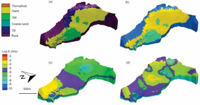
Lemieux et al. 2016). ... 39 Figure 3.3 Precipitation (rain and snow fall) in the study area from October 2012 until October 2016 ... 40 Figure 3.4 Location of pilot-points in the 2D plan. Five layers of pilot-points are used for the 3D model calibration. ... 44 Figure 3.5 a) Hydrostratigraphic units from field investigations, and calibrated hydraulic conductivities from PEST using b) zoning, c) pilot-points and d) pilot-point-zoning

approaches. ... 45 Figure 3.6 Sensitivity of hydraulic head to the hydrostratigraphic units for each observation point. ... 46 Figure 3.7 Comparison between the average observed hydraulic heads at seven

observation wells to the simulated hydraulic heads using the three calibration methods. . 47 Figure 3.8 The respective best and worst fits for the simulated head time series at a) Well 02 and b) Well 04. To better compare the time series and to show the dynamics in head variability, the head time series are adjusted to match observed heads at approximately the start of the observation times. ... 48 Figure 4.1 Location of study area near the village of Umiujaq in northern Quebec, showing observation boreholes and gauging station at the outlet. Red line identifies the cross-section for Figure 4.2. ... 54 Figure 4.2 Cross-section of the study area with 6 distinct hydrostratigraphic units. The location of the cross-section is shown in Figure 4.2. ... 55 Figure 4.3 Measured precipitation and air temperature at Umiujaq from July 2014 to July

(15)

Figure 4.4 Conceptual mesh ... 60

Figure 4.5 Subsurface structure of the 3D model ... 69

Figure 4.6 Calibrated hydraulic conductivities ... 70

Figure 4.7 Simulated flow velocity at the end of the simulation (July 2017) ... 71

Figure 4.8 Simulated hydraulic heads at the end of the simulation (July 2017) ... 72

Figure 4.9 Hydraulic head in the surface water domain at the end of the simulation (July 2017) ... 73

Figure 4.10 Surface water depth at the end of the simulation (July 2017) ... 74

Figure 4.11 Flux exchange between the surface and subsurface domains at the end of the simulation (July 2017) ... 75

Figure 4.12 Simulated and measured hydraulic heads at wells 4, 6 and 9 (in similar intervals as wells 4 and 6, and in full extent) ... 76

Figure 4.13 Simulated water saturation at the three observation wells and the simulated hydraulic head at well 09 ... 77

Figure 4.14 Simulated and measured hydrograph from the model calibration ... 78

Figure 4.15 Calibrated hydraulic conductivity distribution and flow vectors from two models with different numbers of pilot-point layers. The presented cross-sections are not aligned with the flow direction, which means that there can be flow components perpendicular to the cross section. ... 80

Figure 4.16 Comparison of simulated hydraulic heads under steady-state conditions using two pilot-point-zoning models against the observed values ... 81

Figure 4.17 Sensitivity of hydraulic heads at observation wells to the hydraulic conductivity of each hydrostratigraphic unit, in the steady-state simulation ... 83

(16)

Figure 4.19 Comparison between the sensitivity results for hydraulic head at well 02 in the upstream part of the catchment and for hydraulic head at well 04 in the downstream part, using the transient simulation. ... 85 Figure 5.1 Catchment boundary and location of measurements. The red line shows the location of the vertical cross-section A-A’ shown in Figure 5.3. ... 91

Figure 5.2 Measured air temperature, precipitation, and average land surface temperature in Umiujaq for the period of 6th July 2014 to 5th July 2017 ... 92 Figure 5.3 Vertical cross-section A-A’ showing the hydrostratigraphic units (Fortier et al., 2019). ... 93 Figure 5.4 Location of surface probes and fictitious observation points ... 94 Figure 5.5 Boundary conditions applied for heat transport and water flow simulations. .... 97 Figure 5.6 Simulated results showing a) temperatures and b) relative temperature changes (see Eq 5-1) at the three model observation points (SP1, SP2 and SP3) for scenarios IC+5 (red), IC-5(blue), and ICProfile (green)... 101 Figure 5.7 Simulated temperatures at ShallowP and DeepP for scenarios IC-5, IC+5, and ICProfile. ... 103 Figure 5.8 Relative change in energy stored for the different scenarios, as well as surface temperature. ... 104 Figure 5.9 Persistence of the effect of initial condition for IC-5 and IC+5. ... 105 Figure 5.10 Simulated temperatures for scenario ICSpin at three observation locations for the period 6th July 2014 to 5th July 2017. ... 106 Figure 5.11 Observed and simulated temperature profiles in March (cold month) and September (warm month) 2015 and 2016 at T1 and T2 for IC-5, IC+5, ICProfile, and ICSpin. ... 108 Figure 6.1 The Study area is located in a valley close to the village of Umiujaq. Seven

(17)

discharge at the outlet provide the observation data for the field studies. Wells 2 and 3 are close together. The red line shows the cross-section of Figure 6.2. ... 112 Figure 6.2 The study area consists of 6 distinct hydrostratigraphic units. Refer to Figure 6.1 for the location of the cross-section (Modified from Lemieux et al. 2016). ... 113 Figure 6.3 Location of installed probes to measure soil temperature in the catchment ... 115 Figure 6.4 Observed precipitation and air temperature in the study area from 2012-10-01until 2015-07-10. ... 116 Figure 6.5 Temperature data used in the study. Average surface temperature obtained from temperature probes (T(1)), average surface temperature obtained from air

temperature using N factor (T(2)) and three surface probes were used in model scenarios 1, 2 and 3, respectively. ... 119 Figure 6.6 N-factors used for Umiujaq (Buteau, 2002) ... 120 Figure 6.7 The effect of different surface boundary conditions on temperature profile at a) station T1 b) station T2, and c) station T2 in mid September and mid March as the result of applying the N-factor to air temperature (model AirTemp), average temperature measured by probes (model AveSTemp), temperature in the closest probe to the station (model DistSTemp). ... 123 Figure 6.8 Simulated water saturation near station T3 in the variably-saturated model. The black outlines identify three permafrost units near station T3 (vertical exaggeration of 1:3, cross section: X=306990m). ... 125 Figure 6.9 Simulated temperatures (°C) near station T3 in the variably-saturated model (vertical exaggeration of 1:3). ... 126 Figure 6.10 Simulated temperature (°C) near the station T3 in the fully-saturated model (vertical exaggeration of 1:3). ... 127 Figure 6.11 Simulated hydraulic and thermal conditions in July 2017 a) location of the AA’ cross-section at Y=6268750 m, b) hydrostratigraphic units, c) hydraulic heads, d) velocity,

(18)

Figure 6.12 Predicted subsurface temperatures from 2017 to 2047 along section AA’. Since the model is 3D, some of the flow paths cross the section. ... 129 Figure 6.13 Predicted temperature distribution in July from 2017 to 2047 (magnified images). The original extent of permafrost is outlined in black. ... 131 Figure 6.14 a) Location of the longitudinal cross-section (BB') at x=306800 m, b)

subsurface structure c) detailed figure showing the cross-section between y=6268850 m and y=6269250 m ... 133 Figure 6.15 Predicted subsurface temperatures from 2017 to 2047 along section BB’ and between y=6268850 m and y=6269250 m. ... 134 Figure 6.16 Velocity vectors for cross-section BB' after 30 years of simulation (2047). A uniform velocity vector length is used to better highlight the direction of flow. ... 134 Figure 6.17 Effect of climate warming on the predicted subsurface temperature profiles, at the three temperature stations T1, T2 and T3. ... 135

(19)

(20)

Acknowledgment

This has been a long journey, in which I have met many amazing people who helped me to accomplish my PhD. I am extremely grateful to everyone who helped me in this path. I would like to express my deepest appreciation to my supervisor, Prof. René Therrien, for his generous support, expert guidance, and constructive advice. His kindness and continuous support have made my PhD experience one of the best and memorable stages of my life. I have been fortunate to have had this opportunity to work under his supervision. My success in the completion of my dissertation would have not been possible without his support…Thank you René, for everything.

I would like to extend my sincere thanks to my co-supervisor, Prof. John Molson, for his valuable advice and professional feedback and reviews throughout this PhD and in writing of this dissertation.

Many thanks to the external examiners on my doctoral dissertation committee: Prof. Alain Dassargues, Prof. Jasmin Raymond, and Prof. Claudio Paniconi for providing valuable comments and constructive questions.

I am also grateful to Prof. Jean-Michel Lemieux and Prof. Richard Fortier, who have shared their expert knowledge and experience about hydrogeology of Umiujaq, which was significantly helpful to complete this research.

I would like to acknowledge the help of PhD and MSc students who provided field observation data and shared their experiences about Umiujaq, including David Banville, Renaud Murray, Sophie Dagenais, and Dr. Marion Cochand.

Many thanks to my friends and officemates who helped to sustain a positive atmosphere and made my study more enjoyable, including Vinicius Ferreira Boico, Jonathan Fortin, Alexandra Germain, Pierrick Lamontagne-Hallé, and Shuai Guo.

I would like to acknowledge the assistance of the staff of the Department of Geology and Geological Engineering, including Marie-Catherine Talbot Poulin, Pierre Therrien, Guylain Gaumond, Marcel Langlois, and many others.

(21)

I cannot begin to express my thanks to my parents and my sisters for their unconditional love and unwavering belief in me, which always gave me the confidence to overcome the challenges and move beyond what I thought I could.

Above all, I would like to thank my love and husband, Dr. Amir Bolouri, for his endless love, support, and patience, which helped me to pursue my study and get to this point. Thank you for being my editor, proofreader, and sounding board. But most of all, thank you for being my best friend.

(22)

Avant-propos

Chapter 3 of this thesis is an article published by the Canadian Geotechnical Society and presented at the GeoOttawa 2017 conference. The work described in this article was performed during my Doctoral degree at Laval University, under the supervision of Prof. René Therrien and Prof. John Molson. The article describes the initial stage of my PhD research project, involving development and calibration of the water flow model. My role was to develop the 3D model and calibrate it using the available field data. I wrote the manuscript with advice from Prof. René Therrien and Prof. John Molson. The field data used to calibrate the model were obtained by the research team under the supervision of Prof. John-Michel Lemieux and Prof. Richard Fortier and with help from Marie-Catherine Talbot Poulin and Michel Ouellet. Pierre Therrien helped in developing the 2D mesh of the model, which then was transformed to a 3D mesh. The article and the co-authors are as follows:

Parhizkar, M., Therrien, R., Molson, J., Lemieux, JM., Fortier, R., Talbot Poulin, MC., Therrien, P., & Ouellet, M. (2017) An Integrated Surface-Subsurface Flow Model of the Thermo-Hydrological Behavior and Effect of Climate Change in a Cold-Region Catchment in Northern Quebec, Canada. GeoOttawa 2017: the 70th Canadian Geotechnical Conference and the 12th Joint CGS/IAH-CNC Groundwater Conference, Canadian Geotech Soc, Ottawa, 1-4 Oct. 2017.

(23)

Introduction

Background and motivation

Climate change is having a significant impact on ecosystems, economies and communities as well as on subsurface thermal regimes. Climate change can increase groundwater and soil temperatures, which can affect groundwater quality, harm groundwater-sourced ecosystems, and contribute to the geotechnical failure of infrastructure.

Various studies have been conducted to evaluate the effect of climate change on groundwater resources. For example, Menberg et al. (2014) investigated groundwater temperature response to recent climate change. They examined the coupling of atmospheric and groundwater warming with stochastic and deterministic models. Their findings demonstrated that shallow groundwater temperatures have responded rapidly to climate change, thus providing insight into the vulnerability of aquifers and groundwater-dependent ecosystems to future climate change. Lemieux et al. (2015) applied the finite-element model FEFLOW to quantify the potential impact of climate change on freshwater resources of the Magdalen Islands, Quebec, by simulating variable-density flow (induced by saltwater intrusion) and solute transport under saturated-unsaturated conditions. Simulation results showed that the most important impact on groundwater would be caused by sea-level rise, followed by decreasing groundwater recharge and coastal erosion.

Groundwater systems are expected to respond to climate change in a complex way (Bloomfield et al., 2013). Since groundwater supplies almost half of the global drinking water demand (Van der Gun, 2012), investigating the impact of climate change on groundwater temperature and quality is a high priority.

However, further studies are required to better quantify groundwater response to climate change in cold areas. The increase in atmospheric temperature resulting from climate change can lead to permafrost thaw in high altitude and/or high latitude regions. Permafrost is a soil or rock formation that remains at or below the freezing point of water for two or more consecutive years (Dobinski, 2011). Water in the pores of these soils is therefore stored as ice and is essentially immobile and not recoverable by pumping. In addition, permafrost acts as a frozen impervious layer that limits recharge of underlying aquifers, thus decreasing the

(24)

The spatial distribution of permafrost is controlled by several factors including air temperature, vegetation and land surface slope (Shur and Jorgenson, 2007; Jorgenson et al., 2010). According to the Intergovernmental Panel on Climate Change (IPCC, 2007), anticipated climate warming at high latitudes will cause thawing of permafrost over the coming decades. Water trapped as ice will be released and aquifer recharge will increase, which will also likely increase the potential for exploitation of groundwater as a source of drinking water. It is notable that climate change is projected to be most severe at high latitudes, leading to decreasing sea ice, permafrost warming or degradation, increasing carbon dioxide release from soils, decreasing glacier ice mass, and shifting biological indicators (Kurylyk et al. 2014a).

Several studies have been conducted over the past few years to survey the effect of climate change on subsurface conditions in northern regions, including temperature, permafrost distribution, and water quality. The hydrology of the active layer, which is the top layer of soil above permafrost that freezes and thaws on an annual basis, was studied by Quinton and Baltzer (2013) for a thawing peat plateau in a wetland-dominated zone of discontinuous permafrost. Results showed that permafrost thaw reduced subsurface runoff by lowering the hydraulic gradient, increasing the active layer thickness and, most importantly, reducing the surface area of the thawing peat plateau. Wu et al. (2015) investigated changes in active-layer thickness and near-surface permafrost between 2002 and 2012 at 10 sites within five alpine ecosystems. All sites showed an increase in active-layer thickness and near-surface permafrost temperature. They suggested that the primary control on the active-layer thickness increase was an increase in summer rainfall and the primary control on increasing permafrost temperature was probably the combined effects of increasing rainfall and the asymmetrical seasonal changes in subsurface soil temperatures.

Integrated surface and subsurface hydrologic models are valuable tools to understand and characterize catchment functions and behaviour. The following sections will review the available literature for integrated simulations of surface water/ groundwater flow and coupled water flow and heat transfer simulations. Missing gaps in previous research studies are then discussed and the objectives of this study are defined to fulfill some of this missing knowledge.

(25)

Literature review

Integrated simulations for groundwater flow

The terrestrial portion of the water cycle is only one of the many inter-connected components of the complete water cycle. Simulations of catchment-scale groundwater processes are therefore moving towards integration. In an integrated simulation framework, groundwater, surface water and other environmental components are considered as one system. When environmental processes are simulated separately, usually some important assumptions and simplifications are made, which potentially increases the error and uncertainty in the results. Integrated simulation of environmental processes can help to reduce these potential errors.

Integrated simulation of surface and subsurface flow has been used, for example, to study the process of runoff generation (Frei et al. 2010, Liggett et al. 2015, Park et al. 2011, Weill et al., 2013). Ala-aho et al. (2017) applied the HydroGeoSphere model (HGS) for integrated surface-subsurface hydrological simulations to study the role of groundwater in headwater catchment runoff generation. They used a novel calibration approach, which included the main hydrological parameters and minimal field data to simulate the main characteristics of runoff generation. They showed that the model output in an integrated simulation is sensitive to surface parameters as well as subsurface parameters. Therefore, the surface parameters, such as Manning’s coefficients, are appropriate to include in the calibration. Furthermore, they showed that adding observational data improved the model calibration for some output targets, for example groundwater levels, but not for other targets such as evapotranspiration time series.

Jones et al. (2008) applied the Integrated Hydrologic Model (InHM) to a 75-km2_watershed

in southern Ontario to investigate the model’s ability to simulate transient flow processes. They initially calibrated the subsurface flow properties to observed steady-state hydraulic heads and baseflow. They then simulated the stream hydrograph by applying two rainfall time series and compared them to the observed rainfall-runoff responses. Results showed that the model could realistically simulate the fully integrated surface/variably-saturated subsurface flow system.

(26)

The model reproduced the magnitude, temporal variability and spatial distribution of water fluxes at the GW-SW interface. The results were compared to those obtained from airborne measurements of thermal infrared radiation and from mass balance based on stable isotope (18O) data. The general pattern of GW inflow locations to lakes, interpreted from areal thermal imaging, was captured by the simulations, and the GW flux to lakes calculated with the stable isotope technique showed good agreement with the simulations, including reasonable estimates of the hydraulic head and stream baseflow distribution throughout the aquifer. The differences between simulations and observations were mainly attributed to difficulties in observing GW inflow locations with thermal imaging data, model mesh resolution, and a simplified geological model, which led to overestimation of hydraulic head. They concluded that, since field methods for studying transient influxes in a lake system would be labour-intensive, developing a model to reproduce the discharge locations and flow volumes is useful.

Hwang et al. (2018) used HGS to study the effect of parameterization of peatlands and forestlands for a basin-scale simulation of surface-subsurface water flow, in the northern Athabasca River Basin in Canada. They used this model to identify the cause of higher annual downstream flow rates compared to upstream.

El-Zehairy et al (2018) used the MODFLOW-NWT code (MODFLOW with a new Newton (NWT) solver) to characterize the dynamics of transient interactions between artificial lakes and groundwater. They showed that, due to large and fast man-induced changes of lake stages, the interaction of artificial lakes and groundwater is not mainly driven by natural forces (for example precipitation and evapotranspiration) but by a transient balance between river inflow and outflow. They concluded that the study of dynamics between artificial lakes and groundwater requires a fully-coupled model that accounts for variably-saturated flow and for the spatio-temporal variability of water exchange between the surface and subsurface.

Integrated models also create a useful framework to simulate observed catchment behaviour and test future scenarios and potential hydrologic behaviours. For example, Huo et al. (2016) developed an interactive interface between the Soil and Water Assessment tool (SWAT) and MODFLOW to couple surface water-groundwater flow. They applied the integrated model to study the effect of future climate change on river runoff in the Xi’an Heihe

(27)

Yang et al. (2015) used HGS to investigate a 3D heterogeneous coastal aquifer of the Weser river estuary in the German Bight. They studied the long-term impact of climate change considering interactions between mean sea level rise, river discharge variation into the sea estuary and increases of storm surge intensity that induce seawater overtopping. Furthermore, they utilized the software package PEST (Doherty et al., 2010) for the steady-state calibration. Results showed a rise in groundwater level, as well as the creation of surface water ponding and shifts in salinized areas. Moreover, discharge canals cause the seawater to flow further inland by providing pathways for water flow.

Thompson et al. (2015) used an empirical dataset to develop numerical models capable of representing the dominant hydrologic processes, and addressed how catchment hydrology within a complex pond-peat land region is influenced by the configuration of landscape units. They developed 2D models in HGS to reproduce observed hydrologic responses to climate change and to evaluate the sensitivity of the system to changes in specified parameters and boundary conditions. Their results demonstrate a dynamic interaction between pond-peat lands, especially with frequent reversals in hydraulic gradients in response to rain events. Comparisons between simulated and observed hydraulic heads indicated that the models were able to provide a reasonable representation of the groundwater flow system. However, they suggested that neglecting freezing and thawing in the simulation can produce discrepancies in model outcomes, such as poor representation of hydraulic heads. Wetlands located at high elevations were shown to be heavily reliant on precipitation inputs and are particularly vulnerable to changes in climate.

Jutebring Sterte et al. (2018) used the MIKE SHE model to study the influence of catchment parameters and freeze-thaw processes on surface water-groundwater interactions. They showed that the landscape heterogeneity and sub-catchment characteristics play an important role in the catchment hydrological functioning.

Numerical simulations of coupled groundwater flow and heat transfer

Due to the emergence of advanced groundwater flow and heat transport models, the capability to simulate the subsurface thermal response to climate change in hydrologically complex environments has improved rapidly over the last decade. Harlan (1973) is credited for developing the first coupled groundwater flow and heat transport model that incorporates

(28)

model, MarsFlo, for partially-frozen, partially-saturated porous media. MarsFlo accommodates the range of pressure and temperature conditions of interest in studies of the past or present hydrological system on Mars, which by appropriate input choice can be applied to Earth-related hydrological phenomena. MarsFlo uses the integral finite-difference method to discretize the conservation equations. The discretized air and water balance equations are then solved in a fully-coupled manner with the corresponding discretized energy balance equations. In order to validate the model, they used data from previously published laboratory experiments to probe both the underlying mathematical model and its numerical solution. The simulation demonstrated that the choice of spatial difference for the vapor diffusion term significantly affects the simulation behavior at the interface between an ice-saturated and a partially-saturated grid cell, which can lead to convergence failures for the air component. The simulation adequately reproduced the principal phenomenon observed in the experiment, which was freezing-induced water redistribution (cryosuction). Sjöberg et al. (2013) applied MarsFlo in three warming scenarios to study trends of increasing minimum stream discharge and recession flow characteristics (in particular the recession intercept) across various geological settings of northern Sweden. The study showed that these two streamflow characteristics may not always respond to permafrost thaw. Indeed, they are rather different and potentially complementary in the information they provide with respect to permafrost thawing across the northern Swedish landscape. Minimum discharge occurs during the cold season and thus trends in minimum discharge mainly reflect changes in the deeper groundwater flow pathways under and around permafrost bodies, while changes in the recession flow will be more related to active layer dynamics. Although subsurface temperatures responded quickly to the surficial thermal perturbations, they noted that there was a delay in the melting of subsurface ice.

Another finite element code that has been widely used to solve partial differential equations in two or three dimensions is Flex PDE. This code was used, for example, by Bense et al. (2012) for catchments consisting of a series of linked sub-basins, to evaluate how representations of present-day permafrost conditions impact the evolution of groundwater recharge and discharge driven by permafrost degradation. They considered two scenarios with different initial permafrost and hydrogeological conditions. Their simulations showed that permafrost degradation shifts regional connectivity between basins and increases aquifer storage, which leads to modified space-time trends in groundwater regimes. In their

(29)

high. Therefore, permafrost thaw was in this case controlled by heat diffusion while advective heat flow did not accelerate permafrost degradation. They noted that heat advection can impact transient permafrost distribution when recharge is not limited by effective rainfall, when flow is strongly focused, or when geothermal heat flow anomalies occur. In their studied catchment, the initial distribution of permafrost and shifts in aquifer permeability architecture control the timing and circulation rate of groundwater in aquifers. An increase in sub-permafrost hydraulic head and uptake of water into aquifer storage delays the effects of permafrost degradation on increasing groundwater fluxes, possibly by several decades to centuries.

The U.S. Geological Survey model SUTRA is a coupled finite-element simulation model for saturated-unsaturated, fluid-density-dependent ground-water flow. A modified version of SUTRA was used by McKenzie and Voss (2013) to investigate the interaction between heat conduction and heat advection via groundwater flow with both seasonal ground ice and permafrost. They considered two climate change scenarios (i.e. +1 °C/100 yr and +6 °C/100 yr). By comparing the advection-influenced thaw rate and pattern with the case in which there is no groundwater flow, termed conduction-only, they concluded that the time needed for permafrost to disappear in the advection-influenced case was about one-third less than the time required for complete permafrost loss in the equivalent conduction-only system. For conduction-only thaw, the thinnest parts of the permafrost layer thawed first, which led to permafrost bodies persisting below hilltops. In contrast, the warm recharge water in advection-influenced thaw caused the permafrost to thaw mostly below hilltops with residual permafrost zones remaining in the valley. If the permafrost layer is initially discontinuous, with open taliks (unfrozen zones that are often formed by heat flowing from or towards surface water bodies or heated buildings, Kurylyk et al., 2014a) initially below valley surface-water bodies, the time for total thaw may be further reduced.

Briggs et al. (2014) used SUTRA to investigate mechanisms of permafrost aggradation around shrinking Arctic lakes focusing on ecological feedback. Their simulations demonstrated that emerging shrubs, as a result of lake recession and opening of meadow areas, reduce annual direct short-wave radiation to soil due to summer canopy shading. Furthermore, since shrubs intercept and take up water, they also diminish recharge infiltration (heat advection). They showed that a shrub-driven reduction in recharge has a

(30)

However, they suggested that the new permafrost will eventually thaw based on climate projections.

The impact of climate change on the timing, magnitude and temperature of groundwater discharge was studied by Kurylyk et al. (2014b). They applied a modified version of the SUTRA model to small, unconfined aquifers that undergo seasonal freezing and thawing. The model included surface water and heat balance models and was run by applying downscaled climate scenarios to obtain future projections. The simulations show a potential rise in the magnitude and temperature of groundwater discharge to the adjacent river during the summer months as a result of projected increases in air temperature and precipitation. The thermal response of groundwater to climate change was shown to be dependent on the aquifer dimensions. Furthermore, the results indicated that the probability of exceeding critical temperature thresholds within groundwater-sourced thermal refugia (microhabitats for cold water fishes created due to spatially discrete groundwater discharge and induced riverine thermal heterogeneity) may significantly increase under the most extreme climate scenarios.

Another model in this group, HEATFLOW-SMOKER, is an advanced numerical model for solving complex density-dependent groundwater flow and heat transport problems (Molson and Frind, 2018). The model can be used for applications involving the storage or transport of thermal energy in the subsurface where temperatures remain < 100 °C, including advective-conductive heat transport with phase change and latent heat. The HEATFLOW-SMOKER model has been tested and applied to a variety of systems, including groundwater-surface water systems (Markle et al. 2004, 2006; Kalbus et al, 2007) and for simulating permafrost thaw (Grenier et al., 2018; Albers et al., 2020; Dagenais et al., 2020). Shojae Ghias et al. (2016) developed a 2D coupled water flow and heat transfer model with HEATFLOW/SMOKER to study the effect of climate warming on permafrost degradation at the Iqaluit airport, northern Canada. The model considered both advection and conduction processes. Their results showed that even though thermal advection was not negligible in their study area, thermal conduction was the controlling process for permafrost degradation. Dagenais et al., (2020) applied the model to a 2D cross-section of the Tasiapik Valley near Umiujaq, Quebec, where the discontinuous permafrost is rapidly thawing. They showed that advective heat transport played a critical role in permafrost thaw from above and below the shallow permafrost layer. In a parameter sensitivity analysis of the Dagenais model using

(31)

hydraulic parameters defining the surface and near-surface layers had the most influence on the cry-hydrogeological system behaviour.

Hu et al. (2018) developed a fully-coupled heat transport and groundwater flow model with COMSOL Multiphysics. They used the model to study heat transfer during artificial ground freezing with groundwater flow. They concluded that effective hydraulic conductivity and the saturation of unfrozen water control the heat transfer process during the phase change. Painter et al. (2016) present what is likely one of the most advanced coupled models published to date. They applied the Arctic Terrestrial Simulator (ATS) code to integrate surface/subsurface simulation of thermal hydrology in a region with permafrost. They ran a 100-year 2D model and included phase changes, transitions among different states for the land surface, and topography. They suggest the need to reach an acceptable time step to make feasible large 3D decadal projections.

Current research needs

Groundwater supplies almost half of the global drinking water demand. The main question that motivated this research was to investigate how climate change would affect future availability of groundwater for northern communities. Since subsurface systems respond to climate change in a complex way, simulating this complexity requires a state-of-the-art integrated hydrologic model. Despite the available studies on simulations of coupled groundwater flow, heat transport and freeze-thaw processes in cold regions, most studies do not yet consider all relevant hydraulic and thermal processes. According to Ireson et al. (2013), one of the modelling challenges that need to be addressed is to couple the near-surface freeze-thaw cycles with the underlying unsaturated zone and saturated zone groundwater processes, as well as heat transfer by conduction and advection, taking into account phase change and latent heat during permafrost degradation. Furthermore, with the possible exception of the ATS model (Painter et al. 2016), mostly the existing models do not consider surface processes such as snowpack dynamics and surface water flow. Changes in topography due to thaw settlement of ice-rich permafrost, which provide feedback to surface processes and heat transfer at the air-ground interface, are also usually not considered. All these coupled processes are highly dynamic and nonlinear. Predictive accuracy can be limited due to nonlinearity of these coupled phenomena and the presence

(32)

increases with soil water content, flowing groundwater will promote heat transport and permafrost thaw. Thawing permafrost will release more water, which will in turn promote heat transport, creating a positive feedback loop. Moreover, as permafrost thaw may release sequestered carbon, it can exacerbate the rate of anthropogenic climate change (Tarnocai et al. 2009, Harden et al., 2012).

Even though there is increasing interest in exploring groundwater flow and heat transport, only a limited number of field investigations have focused on groundwater. Therefore, the current models have rarely been calibrated against field data. It is recommended that dedicated groundwater monitoring systems should be established to enable assessment of future climate impacts on groundwater (Bloomfield et al., 2013). The number of field investigations is particularly limited in cold regions, due to their remoteness and higher costs to perform these studies in such environments.

Research objectives and methodology

This study focuses on a small catchment near the Inuit village of Umiujaq in Nunavik, northern Quebec. One of the research needs identified for this study was calibrating the coupled water flow-heat transport model against field data in a cold region. The catchment selected for this study is in the discontinuous permafrost zone where detailed field investigations have been ongoing. The model is calibrated using field data. Field investigations have focused on characterizing the hydrogeological and thermal regimes and they provide valuable observations that can be used to calibrate complex numerical models.

The main aim for this study is to develop and apply a 3D integrated thermo-hydrogeological model to the cold-region catchment of Umiujaq. It represents a unique application of a fully-integrated model to a catchment where a detailed hydrogeological characterization was available, as opposed to an application to a synthetic catchment. Furthermore, this work will address existing scientific gaps in coupled groundwater-heat transfer simulations.

Three objectives were defined for this project: a) investigate a new calibration method for simulating water flow in highly heterogeneous areas (chapter 3 and 4), b) identify spin-up strategies to obtain the initial condition for coupled groundwater flow and heat transfer models (chapter 5), and c) apply the model to the cold region of Umiujaq (chapter 6).

(33)

1. Flow model calibration, including an assessment of different calibration strategies 2. Sensitivity analysis

3. Investigating spin-up strategies for heat transport simulations

4. Assessing the role of the unsaturated zone on heat transfer simulations and temperature changes in the subsurface

The following methodology was used to reach the research objectives. First, the existing geological model for Umiujaq (Fortier et.al, 2020) was used to generate the 3D conceptual model, which consisted of the 3D mesh and hydrogeological model. A numerical flow model was then developed based on the conceptual model, using the HydroGeoSphere code, which is a fully coupled surface-subsurface flow model designed to simulate the coupled water flow-heat transport process. The model included the key components of the hydrologic cycle, including precipitation, infiltration, surface flow, and groundwater flow. Heat transfer processes were then coupled to the water flow model to provide insight and understanding into subsurface thermal dynamics in the study area.

This project addresses some of the deficiencies noted in the previous hydrogeological studies of cold regions. These include coupling surface-subsurface flow in a 3D environment and including the effect of snowmelt and the unsaturated zone. Furthermore, the project benefits from access to detailed hydrogeological field data from a cold region environment, which has been a limitation in previous hydrogeological studies of cold regions.

The present thesis contains six chapters. Chapter 1 presents the study area, near Umiujaq, Canada, and a summary of field measurements. Chapter 2 describes the numerical code, used to simulate coupled flow and heat transport. Chapter 3 is a conference paper presented in GéoOttawa, 2017: 70 years of Canadian Geotechnics and Geoscience. Chapters 4, 5, and 6 present the simulations and results of this study. These chapters are written in the format of journal papers and they will eventually be submitted for publication. Because of the format, there is some repetition in these papers in relation to the site and numerical model description. The last chapter concludes this work and discusses perspectives and potential future research.

(34)

1 Study area

1.1 Location

The study area for this project is located in the Tasiapik valley near the village of Umiujaq in northern Quebec, Canada (56°32′N 76°33′W; Figure 1.1, Figure 1.2). The catchment covers an area of 2.23 km2_{, within the discontinuous permafrost zone.}

(35)

Figure 1.2 Location map of the study area in the Tasiapik Valley near the Inuit village of Umiujaq in northern Quebec

1.2 Geology and hydrogeology

Within the study area, six distinct hydrostratigraphic units were defined by LIDAR topographic surfaces, surface geophysical EM surveys and borehole logs (Figure 1.3). An elevation difference of 100 m exists between the flat downstream part of the valley and the relatively flat upstream area. In the upper reaches of the valley, the surface layer is a thin layer of littoral and pre-littoral sediments, which contains a shallow, perched aquifer. Below this aquifer lies a layer of frost-susceptible silt, which is thinner in the upstream part and becomes thicker downstream. In the frost-susceptible silty marine unit, discontinuous permafrost mounds can be seen in the cross-section, especially where the silty layer is thicker. The silt layer overlies the layers of subaqueous fluvioglacial sediments (Gs) and frontal moraine deposits (Gxt). Units Gs and Gxt form a deeper aquifer that is unconfined in the upper part of the valley and confined in the lower part.

(36)

they are about 50 m in diameter. The active layer, less than 2 m thick, is the surficial layer of the permafrost mound. The permafrost base is about 22.5 m deep (Leblanc et al., 2006). The catchment has a river system that is mainly intermittent except for the main stream. The vegetation cover varies according to the level of drainage. High topographic and well-drained zones in the upstream part of the watershed contain lichen vegetation, whereas convex topographic areas contain shrubs. Spruce vegetation is found in well-drained sites in the southeast part of the watershed and herbaceous plants are found near bodies of water (Provencher-Nolet, 2014).

Figure 1.3 Cross-section of the study area along the valley axis showing 6 distinct hydrostratigraphic units

1.3 Climate

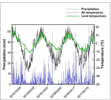
The regional climate of the study site is subarctic with cool and damp summers, and relatively dry and cold winters. Hudson Bay has a major influence on the regional climate due to strong winds in winter over the frozen bay and due to frequent dense fog in summer. A weather station in the catchment measures wind speed, air temperature and precipitation (Figure 1.4). Figure 1.5 shows measured air temperature, precipitation, and land surface temperatures from 2014-05-01 until 2017-05-01. Generally, the cold season occurs between October and May, and above-zero temperatures occur from May to September. The mean annual air and land surface temperatures for this period were -4.5 and 0.6 °C, respectively. The mean annual precipitation between 2014 and 2017, including rain and snow, was 760 mm.

(37)

Figure 1.4 The weather station in Umiujaq (Barrère, 2018)

Figure 1.5 Measured precipitation, land and air temperatures at Umiujaq from July 2014 to July 2017

(38)

1.4 Field investigations and observed data

The hydrology of the catchment has been under investigation since 2013. The physical properties of the geological materials such as hydraulic and thermal conductivities, porosity, and specific heat capacity were measured in the field (Murray 2016, Dagenais 2018). Furthermore, meteorological conditions such as precipitation, thickness of snow cover, and air temperature have also been regularly measured. Several observation stations have been installed in the valley (Lemieux et al. 2020), including a gauging station located at the outlet of the watershed, which quantifies surface runoff in the basin, seven observation boreholes that measure the groundwater level throughout the valley, and 3 temperature stations that measure the temperature profile down to 35 m in depth (Figure 1.6). Furthermore, the land-surface temperature has been monitored with 38 probes installed at a depth of 10 cm throughout the catchment (Figure 1.7). The location of the surface-temperature probes was chosen to include different conditions in the catchment that could affect thermal behaviour, including type of vegetation, depth of snow cover and soil type. Field investigations in the catchment have also included the study of hydro-geochemistry (Cochand et al. 2020). Table 1.1 summarizes the available data from the field investigations.

Table 1.1 Available data provided through field investigations

Category Data Source of Data

Geological

Thickness of sediments Distribution of sediments

Water table elevation and location Permafrost location and thickness

Geophysics (Resistivity) Hydrogeological Data Physical properties (K, θ) Water levels Slug tests

Grain-size or sediment type Observation boreholes

Thermal Data

Thermal conductivity Heat capacity

Temperature depth profiles

Lab measurements Temperature probes Literature values Hydro-

geochemistry Major ions, pH, isotopes

Surface-subsurface sampling

(39)

Meteorological

Air temperature

Precipitation (rain, snow) Snow thickness

Meteorological stations

Banville (2016) and Fortier et al (2020) carried out a cryo-hydrogeophysical investigation of the study area and developed a 3D geological model using GOCAD, which delineated the boundaries of all hydrostratigraphic units in the study area (Figure 1.8). In the current study, grid elements of the numerical model were assigned properties based on this 3D geological model.

(40)

Figure 1.7 Instrumentation at the Umiujaq field site for thermal measurements: Thirty-eight probes are installed at depths of 10 cm to measure the ground surface temperature

(41)

Figure 1.8 3D GOCAD geological model of the hydrostratigraphy in the Tasiapik Valley (Banville, 2016).

1.4.1 Precipitation measurement and processing

The weather station in Umiujaq (Figure 1.4) uses the Geonor T200-B precipitation gauge with an alter windshield to measure hourly precipitation (Smith, 2007). Systematic biases in measurements include wind-induced under-catch, wetting loss, evaporation loss and underestimation of trace precipitation amounts. For example, turbulent airflow over the gauge can prevent precipitation from falling into the bucket, which results in an under-estimation of true precipitation. Wind turbulence, in particular, affects snow catch in the bucket, since snow has lower density and falling speed. Therefore, treatment of the data is sometimes necessary to correct the precipitation (Goodison et al., 1998). In the course of this PhD project, the hourly precipitation measured by the Geonor T200-B gauge in Umiujaq was processed by applying the hourly relationship between wind speed and Geonor gauge catch efficiency. The methodology used to process the observed precipitation data is described here and the applied Matlab code and the steps are presented in Appendix 1. Meteorological data used to process precipitation included hourly measures of air temperature, wind speed, and cumulative total precipitation. The Geonor T200-B unit at Umiujaq had only one vibrating wire until October 2015, when it was upgraded to include

(42)

0.1 mm at hourly intervals. The bucket is emptied twice each year and oil and antifreeze is added to melt frozen precipitation and minimize evaporation from the bucket.

1.4.1.1 Methodology

Measured precipitation at Umiujaq by Geonor T200-B was processed before being used in the numerical model. However, as it will be described in Chapter 4, processing of the precipitation data resulted in precipitation rates that were too high and not in agreement with climate conditions in Umiujaq. Therefore, in the end, the unprocessed precipitation data were used in the model. Nevertheless, the methodology used to process the precipitation data and the results are described in following sections.

1.4.1.1.1 Data pre-processing

The first step is to manually remove obvious outliers and eliminate the effect of gauge maintenance events like emptying the bucket and adding the oil. Subsequently, an automated filtering is needed to remove the effect of evaporation and sublimation (Duchon, 2008). For automatic filtering, a “brute-force” filtering algorithm is used to eliminate negative and small positive values by aggregating them with the nearest positive value, above the specified threshold (Pan et al., 2016). Here a threshold of 0.1 mm, which is the smallest value measureable by the device, is considered as the lowest acceptable measurement and all values below 0.1 mm were eliminated by aggregating them with the nearest acceptable positive value. The “brute-force” filtering algorithm consists of three steps. In the first step, the hourly precipitation, as the difference between consecutive values, is calculated from the cumulative time series recorded by the device. In the next step starting from the lowest off-threshold value, all values below the specified threshold were combined with the nearest positive values and then set to zero. This filtering algorithm assumes that the total cumulative precipitation is correct; therefore, at the end of the filtering process the total cumulative precipitation should be same for the initial and corrected data.

1.4.1.1.2 Correcting for under-catch of precipitation

The catch efficiency of a gauge with an alter wind shield has been shown to decrease with increasing wind speed, resulting in an under-catch of precipitation (Smith 2007). These biases in precipitation measurements are more evident in winter, since snow particles are

(43)

for wind-induced biases is necessary to obtain more realistic precipitation values. A solid precipitation measurement inter-comparison was organized by the WMO in 1985 to introduce a reference method of solid precipitation measurement and to calibrate precipitation gauges (Goodison et al., 1998). Smith (2007) used the reference method recommended by WMO using the Geonor T200-B with an alter windshield to obtain the following empirical relationship between catch efficiency and wind speed:

𝑃𝑐𝑜𝑟= 𝑃𝑜𝑏𝑠/𝐶𝐸 𝐶𝐸 = 1.18𝑒−0.18𝑊𝑠 (1-1) where 𝑃_𝑐𝑜𝑟 (mm) is the corrected precipitation, 𝑃_𝑜𝑏𝑠 (mm) is the measured solid precipitation after filtering, 𝑊𝑠 (ms-1) is the hourly mean wind speed at the gauge height, catch efficiency (𝐶𝐸) is the ratio of the Geonor catch to the “true” snowfall measured by a WMO reference called the double-fence inter-comparison reference (DFIR) (Goodison, et al., 1998). According to Smith (2007), this correction is applicable to a relatively cold, dry, and windy environment such as the Canadian prairies and arctic. Accurate snowfall observations are required in near real time. This relationship for 𝐶𝐸 is obtained for hourly measured precipitation. Therefore, in this project, an hourly timescale is used for the precipitation, wind and temperature measurements.

For a Geonor T200-B located in an open site with short grass:

𝑊𝑠(ℎ) = 𝑊𝑠(𝐻) [ 𝐿𝑛(ℎ 𝑧0) 𝐿𝑛(𝐻 𝑧0) ]

(1-2)

where 𝑊𝑠(ℎ) and 𝑊𝑠(𝐻) are wind speed at gauge height (m/s) and wind speed measured by an anemometer (m/s), respectively, ℎ and 𝐻 are the elevation of the Geonor (1.75 m) and the elevation of the anemometer (10m), respectively, and 𝑧₀ is the roughness (m). It is assumed that the shrubs are completely covered by snow in winter so the roughness is assumed equal to 1 mm for the snow period (𝑇_𝑎< 0) and one-tenth of shrub height (2 cm) for the warm period (𝑇_𝑎> 0).

For rainfall, a 𝐶𝐸 of 95% was measured for the Geonor instrument, relative to the WMO reference pit gauge for rainfall inter-comparison. Therefore, the wind biases for rainfall have not been considered here, and the data were corrected only for snowfall.

(44)

To avoid over correction, a maximum threshold for wind speed has to be assigned. For daily precipitation total, a maximum daily mean wind speed of 6.5 m/s is often applied in Arctic and northern regions (Yang et al., 2005). Furthermore, according to Smith (2007), the 𝐶𝐸 for the Geonor with an alter shield remains equal to 1 at wind speeds up to 1.2 m/s. This is due to elimination of wind turbulence by the shield. Determination of precipitation type is also required for the bias correction algorithm for precipitation measurements, which can be done either by using a specific temperature to separate rain and snow, or by using a specified threshold to also include the mixed rain-snow type. Barrère (2018) has compared two methods for Umiujaq: 1) considering a temperature threshold of 1 °C to distinguish between rain and snow, and 2) including mixed rain and snow for temperatures between 0 and 2°C. However, the resulting cumulative precipitation did not show a significant difference between the two approaches. Therefore, a temperature threshold of 1 °C has been used in this study to separate rain and snow.

1.4.1.2 Results

Measured precipitation by the Geonor T200-B gauge can include noise in the time series. Sources of such noise include electromagnetic disturbances, irregular diurnal drift due to turbulent pressure fluctuations and temperature effects on gauge transducers (which is more evident during cold periods), and an evident decline in accumulation due to evaporation losses (Pan et al., 2016). This noise was removed by applying the filter described in the previous section. Figure 1.9 shows an example of noise in the cumulative precipitation data and corresponding filtering. Although the filtering process can create artificial rainfall events or can remove real events, it will preserve the total accumulation in a year.

(45)

Figure 1.9 Effect of automated filtering to eliminate the effect of noise in the precipitation measurements

Figure 1.10 and Figure 1.11 show the monthly wind-induced bias corrections and the corresponding meteorological summaries, respectively. In summer, when precipitation only occurs as rainfall, the observed and corrected precipitation values are equal since the catch efficiency is considered equal to 1 for rainfall (Figure 1.10). Higher wind speed tends to be correlated to colder weather in winter, which decreases the catch efficiency of the device (Figure 1.11). As a result, corrections can reach up to 198% or 71 mm in winter (Figure 1.10). Bias correction also changes the peak in the annual precipitation cycle from summer to winter. Generally, the largest corrections are for November and December, due to higher wind speed and low temperature.

(46)

Figure 1.10 Monthly bias corrections in the precipitation data at Umiujaq

(47)

The frequency of observed hourly rainfall and snowfall is shown in Figure 1.12. To better highlight the lighter precipitation events, events over 5 mm/h, which occur less frequently, have been removed. The lighter precipitation events (<1 mmh-1_{) occur more frequently than}

heavier precipitation. Also, heavier rainfalls happen more frequently compared to snow events.

Figure 1.12 Histogram of hourly precipitation for a) Rainfall b) Snowfall (a)

(48)

Another phenomenon that can affect measurement of snowfall is blowing snow, which is defined as snow lifted from the surface by the wind. Blowing snow can influence measurements in winter and quantifying its impact is challenging. Blowing snow fluxes collected by precipitation gauges are called false precipitation measurements (Pan et al, 2016). Blowing snow often occurs after continuous high wind speed (

W

_s>9.5 ms-1_{) and may}

increase the volume of measured precipitation up to 50% (Bardsley and Williams, 1997). At this study site, the Geonor gauge is located in an open area. Therefore, the wind turbulence and blowing snow can influence the catch efficiency more than they affect devices with natural shielding of surrounding forests or bushes. Also, at Umiujaq, the elevation difference between the device and the top of the snow decreases in winter (Figure 3). Therefore, blowing snow can cause major errors in the measurements and a more detailed study is needed to quantify the magnitude of over-measurement caused by the blowing snow. Therefore, in this study, the effect of blowing snow is not considered in the processed precipitation.

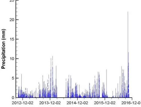
Figure 1.13 shows the hourly wind speed measured at the weather station (see location in Figure 1.4). During the 2012-2016 period, wind speeds greater than 9.5 ms-1 _{were measured}

several times. When they occur in winter, these high winds can generate blowing snow that creates anomalous precipitation readings. From Equation 2-1, a high 𝑊𝑠 results in a smaller value for 𝐶𝐸, which will increase𝑃𝑐𝑜𝑟. Therefore, if the measurement included this erroneous precipitation reading during blowing snow, the use of bias corrections for under-catch will even magnify errors caused by the blowing snow. An example of high wind speed and corresponding bias-corrected snowfall is provided in Figure 1.14 while the raw and corrected precipitation values are provided in Figure 1.15. During the winter, negative precipitation values were recorded by the device, which has reduced the total processed precipitation. These negative values were considerable during the winter of 2014.

(49)

(50)

(51)

Figure 1.15 Raw and corrected precipitation at Umiujaq from October 2012 to October 2017