Modeling and Simulation of Photovoltaic Generator

(1)

HAL Id: dumas-01220257

https://dumas.ccsd.cnrs.fr/dumas-01220257

Submitted on 26 Oct 2015

HAL is a multi-disciplinary open access archive for the deposit and dissemination of sci-entific research documents, whether they are pub-lished or not. The documents may come from teaching and research institutions in France or abroad, or from public or private research centers.

L’archive ouverte pluridisciplinaire HAL, est destinée au dépôt et à la diffusion de documents scientifiques de niveau recherche, publiés ou non, émanant des établissements d’enseignement et de recherche français ou étrangers, des laboratoires publics ou privés.

Ngoc Ban Nguyen

To cite this version:

Ngoc Ban Nguyen. Modeling and Simulation of Photovoltaic Generator. Electric power. 2014. �dumas-01220257�

(2)

MASTER THESIS

By:

Nguyen Ngoc Ban

Energy Department

Title:

Modeling and Simulation of Photovoltaic Generator

Supervisor:

Prof. Stéphan ASTIER

Laboratory on Plasma and Conversion of Energy

(3)

Nguyen Ngoc Ban Page 2

ACKNOWLEDGEMENT

The work presented in this report was performed during the six months final internship of USTH Master “Energy – Green Electricity”, for Master Thesis, at the Laboratory on Plasma and Conversion of Energy (LAPLACE), in “Groupe Energie Electrique et Systémique” (GENESYS) research team located in the École Nationale Supérieure d’Electrotechnique, d’Electronique, d’Informatique, d’Hydraulique et des Télécommunication (ENSEEIHT). After six months of research, I would like to thank all those who helped me by contributing to the success of this work, especially:

 Professor Stéphan ASTIER, lecturer at ENSEEIHT, who is my internship supervisor for his indispensable instruction to guarantee the success of my works and this report.

 Director of research at CNRS Xavier Roboam for welcoming me in GENESYS research team.

 Ms. Fatima Zahra El Alya, a student at University Toulouse III-Paul Sabatier, who gave me the first concept of MATLAB SIMULINK.

 Mr. Redouane, Mr. Tony and Mr. Ulises, students at ENSEEIHT, who are my roommate for their enthusiastic help.

I would like to thank my university USTH and the LAPLACE for giving me a chance to work in France. It was a great experience with new friends, new working environment and new ways of thinking. Finally, I would like to thank my family, and my friends in Viet Nam and Toulouse, particularly Mr. Quynh, Mr. Hung and Mr. Thi for their belief in me and indispensable help.

15th, August 2014 Nguyen Ngoc Ban

(4)

CONTENT

ACKNOWLEDGEMENT ... 2 LIST OF FIGURES ... 5 LIST OF TABLES ... 6 ABBREVIATIONS ... 6 ABSTRACT ... 7 INTRODUCTION ... 8

CHAPTER I: SOLAR ENERGY AND PHOTOVOLTAIC CELL ... 9

1.1. Solar energy ... 9

1.1.1. Introduction ... 9

1.1.2. Advantage and disadvantage of solar photovoltaic ... 9

1.1.3. Potential of solar photovoltaic ... 10

1.1.4. Photovoltaic installations at LAPLACE on LABEGE and ENSEEIHT sites ... 10

1.2. Photovoltaic cell ... 11

1.2.1. Photovoltaic working principles ... 11

1.2.2. Modeling of Photovoltaic devices ... 12

1.2.2.1. Ideal photovoltaic cell ... 12

1.2.2.2. Practical photovoltaic cell ... 13

1.2.2.3. Photovoltaic module and arrays ... 14

1.2.2.4. Global approach ... 16

CHAPTER II: SIMULATION OF PHOTOVOLTAIC GENERATOR AND MAXIMUM POWER POINT TRACKING ... 18

2.1. Simulation of photovoltaic generator ... 18

2.1.1. Photovoltaic module ... 18

2.1.2. Photovoltaic modules in series ... 21

(5)

2.2. Maximum power point tracking ... 24

2.2.1. Perturbation and observation ... 26

2.2.2. Sweeping technique with voltage regulation ... 29

CHAPTER III: SIMULATION OF PHOTOVOLTAIC EMULATOR ... 32

3.1. Objective ... 32

3.2. Structure of a photovoltaic emulator ... 32

3.3. Photovoltaic emulator in SIMULINK ... 33

(6)

LIST OF FIGURES

Figure 1.1: Annual photovoltaic installation (W.Arnulf, 2013) ... 10

Figure 1.2: Working principle of a PV cell ... 11

Figure 1.3: Equivalent circuit of a PV cell (a) Ideal, (b) with series resistance Rs, (c) with series and parallel resistance, Rs and Rsh, (d) with two diodes ... 13

Figure 1.4: Photovoltaic cell, module and arrays ... 15

Figure 2.1: I-V curve of 1 module E20 ... 21

Figure 2.2: P-V curve of 1 module E20... 21

Figure 2.3: I-V curve of 2 modules E20 in series without diode bypass ... 22

Figure 2.4: P-V curve of 2 modules E20 in series without diode bypass ... 22

Figure 2.5: I-V curve of 2 modules E20 in series with diode bypass ... 22

Figure 2.6: P-V curve of 2 modules E20 in series with diode bypass ... 22

Figure 2.7: I-V curve of 2 modules E20 in parallel without blocking diode ... 23

Figure 2.8: P-V curve of 2 modules E20 in parallel without blocking diode ... 23

Figure 2.9: I-V curve of 2 modules E20 in parallel with blocking diode ... 24

Figure 2.10: P-V curve of 2 modules E20 in parallel with blocking diode ... 24

Figure 2.11: Maximum power point at different condition ... 26

Figure 2.12: Perturbation and observation method ... 27

Figure 2.13: Perturbation and observation flow chart ... 28

Figure 2.14: Photovoltaic system including MPPT and DC-DC converter ... 30

Figure 2.15: P&O method ... 31

Figure 2.16: Sweeping method ... 31

Figure 3.1: Principle and structure HIL of the PV emulator ... 33

Figure 3.2: Power curve of PV model and emulator in case 1 ... 34

Figure 3.3: Power curve of PV model and emulator in case 2 ... 34

Figure 3.4: Structure of photovoltaic emulator in case 3 ... 35

Figure 3.5: Power curve of PV emulator with analog low pass filter (C = 2.2e-3F) ... 36

(7)

LIST OF TABLES

Table 2.1: Quality diode factor dependent on PV technology ... 19 Table 2.2: Comparison of manufacturer’s data with results of the simulation... 21 Table 2.3: Comparison of the results ... 29

ABBREVIATIONS

DC ENSEEIHT EPBT GENESYS HIL INPT LAPLACE P&O PEM PV Direct Current

École Nationale Supérieure d'Électronique, d'Électrotechnique, d'Informatique, d'Hydraulique et des Télécommunications

Energy Payback Times

Groupe Energie Electrique et Systémique Hardware in The Loop

Institut National Polytechnique de Toulouse Laboratory on Plasma and Conversion of Energy Perturbation and Observation

Proton Exchange Membrane Photovoltaics

(8)

ABSTRACT

A modeling and simulation of photovoltaic (PV) arrays is necessary to study the behavior of a photovoltaic (PV) system without effect of outdoor weather conditions. This report used PV equivalent circuit with one diode, series resistance and parallel resistance and MATLAB SIMULINK to simulate it with different situations such as associating with bypass diode, blocking diode, maximum power point tracking and static converter. Besides, a modeling and simulation of photovoltaic emulator also is presented in the report. The emulator use electricity from main grid and provide output current and output voltage like a real PV module. The results are reasonable with theoretical studies and will be validated when real PV systems are mounted in ENSEEIHT and LABEGE.

Key words: Photovoltaics (PV), MATLAB SIMULINK, Modeling, Simulation, Maximum Power Point Tracking (MPPT), Emulator.

TÓM TẮT

Một mô hình hóa và mô phỏng của các dãy pin mặt trời là cần thiết để nghiên cứu hành vi của một hệ thống pin mặt trời mà không chịu ảnh hưởng của điều kiện thời tiết bên ngoài. Báo cáo này đã dụng mạch tương đương với một diode, điện trở nối tiếp và điện trở song song và MATLAB SIMULINK để mô phỏng nó với những tình huống khác nhau như kết nối với bypass diode, blocking diode, bộ dò tìm công suất cực đại và bộ biến đổi tĩnh. Bên cạnh đó, mô hình hóa và mô phỏng của PV emulator cũng được trình bày trong báo cáo này. Emulator sử dụng điện từ mạng điện và cung cấp dòng điện và điện áp đầu ra giống như một module pin mặt trời thật. Các kết quả là phù hợp với các nghiên cứu lý thuyết và sẽ được kiểm chứng khi các hệ thống pin mặt trời thật được lắp đặt ở ENSEEIHT và LABEGE.

(9)

INTRODUCTION

The continuous development of population and particularly industrial sector push the demand of energy and it make the role of energy become more and more important and being an indispensable element in life. However, present used forms of energy are primary from fossil fuels (oil, gas, and coal) and they are depleted, become scarce and have bad impact on environment and health of people.

In this context, solar energy is one of the keys to solve these problems. The evolution of technology facilitates this inexhaustible, clean energy source come to customers with lower price and higher efficiency. In order to support theoretical studies, the LAPLACE is going to mount photovoltaic generator systems with different PV cell technologies on the lab roof. These strings are expected to be connected to batteries and to a hydrogen storage system. PEM fuel cells consuming the stored hydrogen will generate electricity supplying the load and grid both with solar panels and batteries. The aim is to realize a flexible micro-smart-grid emulator by interconnecting these devices.

In this context, it is significant to develop models and simulators of every component used in order to perform simulations of different types of architectures with the aim of being able to compare simulations and experiments. Doing this for the different kinds of photovoltaic cells, strings and generators used was particularly my job during my internship. By understanding mathematical equations of a photovoltaic cell and using MATLAB SIMULINK, a simulator of strings which will be installed on the roofs of two laboratory’s sites, site ENSEEIHT and site LABEGE has been developed and validated.

In this thesis report, there are three main parts: Chapter I: Solar energy and photovoltaic cell

Chapter II: Simulation of photovoltaic generator and maximum power point tracking Chapter III: Simulation of emulator

(10)

CHAPTER I: SOLAR ENERGY AND PHOTOVOLTAIC CELL

1.1. Solar energy

1.1.1. Introduction

Solar energy is one of the most potential renewable energy sources to solve the energy shortage at present and particularly in future when fossil fuels are getting exhausted. It can be used for heat and electricity. For heat, solar water heaters can cover 60% to 90% demand of household hot water in Vietnam for example and therefore it reduces electric consumption for hot water (J.Nicolas, 2013). For electricity, solar photovoltaic systems can transform sunlight into electricity with different efficiencies correspond to various technologies. At the moment, the investment cost of one this system is quite high, but the development of technology and electric deficit will make solar panels more significant.

1.1.2. Advantage and disadvantage of solar photovoltaic

None of energy sources is perfect, so solar photovoltaics also has its pros and cons. Hereafter are given some main advantages and disadvantages of it.

Disadvantages:

 It is daily intermittent with the night and shading conditions by clouds or natural and artificial reliefs, with seasonal variations depending on latitude; thus it needs an expensive electric storage system and/or complementary sources.

 Initial investment cost is relatively high at the moment and a large space is required for installing because of its low power surface density.

 Fabricating process is itself energy hungry and involves in toxic chemical substances. Advantages:

 This is a clean, inexhaustible and abundant energy source which delivers electricity without noise, pollution and moving parts in working process, with a very great reliability.

 It can be operated with or without national grid connection, so it is suitable for distributed generation, islands and remote areas where there is no electric grid.

 Conversion ratios from light to electricity are increasing while energy payback times (EPBT) and costs are decreasing due to the development of new technologies.

(11)

Nguyen Ngoc Ban Page 10  It can work well for more than 20 years with very small reduction of efficiency per

year.

1.1.3. Potential of solar photovoltaic

In the context of energy shortage, solar photovoltaics become more and more important with every country. The annual growth rate of photovoltaic industry production is approximate 55% over the last decade (W.Arnulf, 2013) and it demonstrates that this industry has a large potential.

Figure 1.1: Annual photovoltaic installation (W.Arnulf, 2013)

1.1.4. Photovoltaic installations at LAPLACE on LABEGE and ENSEEIHT sites

The promising of solar PV in future attracts many research centers including the LAPLACE in which searchers have been developing PV systems for more than 30 years. In October 2014, the lab will install 2 PV systems coupling with hydrogen storage on the roofs of site ENSEEIHT and site LABEGE (at INPT). Two these systems will provide electricity for the buildings but mainly enable experiments of behavior of different micro smart grid architectures including hydrogen storage, a very promising solution. The structures of the two generators made of 4 strings (PV_N1, PV_N2, PV_N3 and PV_N4) in site ENSEEIHT and 3 strings (PV_I1, PV_I2, PV_I3) in site LABEGE are presented in figure A.1 and A.2 in

(12)

appendix A. For flexible experiments, strings, each of different technologies, can be used separately or connected together with various architectures.

In order to test in virtual the behavior of these various possible smart grids, a model of temperature and irradiation have been achieved and to continue the task it requires a model and simulation of PV strings. Therefore, I take responsibility of making it so that the PV model will be validated when real devices come into operation.

1.2. Photovoltaic cell

1.2.1. Photovoltaic working principles

Basically, a Photovoltaic (PV) cell is a semiconductor device which converts directly sunlight into electricity. The cell includes three main parts: a semi-conductor P-N junction with an antireflection coating facing the light and a metallic contact to connect an external electric circuit (http://www.pveducation.org/pvcdrom).

Solar light energy is composed of photons with different wavelengths, in the other words with different energies. As shown on fig 1.2, when a PV cell is exposed to sunlight, it absorbs some of the photons (optical capture). Photons with energy lower than band gap of semiconductor material of the cell are unusable and cannot produce any voltage or electric current. Photons with energy higher than this band gap are usable and generate electricity,

Figure 1.2: Working principle of a PV cell

but only the energy equal the band gap is productive, the rest is lost, dissipated as heat and make the cell become hotter (M.Villalva, R.Jonas, & R.Ernesto, 2009) . The energy from photons excite electrons of atoms to jump from valence into conduction band: pairs of free electrons and holes are created. Under the effect electromagnetic field of P-N junction, free electrons and holes move in opposite directions generating a photocreated current. A part of these electrons are collected by thin metallic grid on the surface of the cell injected in the

(13)

external load to come back the cell and combine with holes. Both electric current and voltage are formed, i.e. electric power (part of incoming light power) able to supply an external load.

1.2.2. Modeling of Photovoltaic devices

1.2.2.1. Ideal photovoltaic cell

Considering the presented physical principles of photovoltaic conversion an ideal photovoltaic cell can be presented by an equivalent circuit as figure 1.3a. It includes an ideal diode connected in parallel with ideal current source representing the photocreated current IL (M.Villalva et al., 2009).

The basic equation for output current of an ideal PV cell:

0 . [exp( ) 1] . . L d L I I I q V I I I A k T      Where:

I: Output current of the PV cell (A) V: Output voltage of the PV cell (V) IL: Photocreated current (A)

I0: Reverse saturation current of the diode (A)

q: Electron charge (1.602 e-19 C) k: Bolzmann constant ( 1.380 e-23 J/K) T: Temperature of the P-N junction (Kelvin) A: Quality diode factor

(14)

Figure 1.3: Equivalent circuit of a PV cell (a) Ideal, (b) with series resistance Rs, (c) with series and parallel resistance, Rs and Rsh, (d) with two diodes

1.2.2.2. Practical photovoltaic cell

More accurate equivalent circuit of a PV cell can be presented as figure 1.3c and figure 1.3d. It depends on accuracy level that each authors desire. In a real PV cell, there are some contacts between thin metallic grids on the top of the cell, metallic base at the bottom with N layer and P layer respectively and other contacts that cause power loss. These additional losses and other ones due to dissipative phenomena and technology realization are globally modelled by means of Rs and Rsh. The figure 1.3d gives a model better than model in figure 1.3c considering recombination, but the most difficulty of the model in figure 1.3d is to get the data of parameters. Therefore, the model in figure 1.3c is used more for modeling and simulation of PV generator. It is simpler, but the accuracy is still acceptable.

Equation of output current with figure 1.3c (M.Villalva et al., 2009):

0 .( . ) . [exp( ) 1] . . L d Rsh L I I I I q V I Rs V I Rs I I I A k T Rsh          Where:

(15)

Rsh: Shunt resistance of a PV cell (Ω)

Equation of output current with figure 1.3d (Piazza & Vitale, 2013):

1 1 L d d Rsh I  I I I I With: 1 01 2 02 .( . ) [exp( ) 1] . .( . ) [exp( ) 1] 2. . d d q V I Rs I I k T q V I Rs I I k T      

1.2.2.3. Photovoltaic module and arrays

Due to output current and output voltage of a PV cell is small, so PV cells are connected in series to increase output voltage and in parallel to raise output current. This set of cells is called a module. A typical module includes 36 cells or 72 cells series connected in order to produce a voltage over 12V or 24 respectively.

To raise output power, PV modules are associated into arrays. In this structure, the modules can be connected in series, in parallel or both of them.

In practical, actual properties of cells and environmental conditions (illumination, shadowing, and temperature) cannot be uniform on arrays in such association with large number of cells, so that unbalance effects appear in the network. It results in a global power decreasing (because in a series association, a cell delivering the lowest current imposes the output current) or even reverses polarizations and hot spots which can destroy shadowed cells. In typical mounting, bypass diodes for each module and series diodes for each leg, as shown on fig 1.4 c, prevent from any of these problems by spontaneous switch-on, isolating the weaker modules when necessary.

(16)

Figure 1.4: Photovoltaic cell, module and arrays

In normal operating conditions, without any diode switched-on, a PV array is considered with Ns cell connected in series and Np parallel connection of cells (legs) so that:

. . tot P tot S I N I V N V    _ 

In my work, I use the model of practical PV cell with one diode as figure 1.3c. With this model we have:

0

.( . ) .

( [exp( ) 1] )

. .

tot tot tot tot

S P S P tot P L V I V I q Rs Rs N N N N I N I I A k T Rsh       L

I is influenced by the temperature and solar irradiation. Considering given data (Iscn, Vocn) for standard test conditions (G=1000 W/m2, T=298 K), the photon current of a PV cell can be calculated by equations taking account of irradiation and temperature (M.Villalva et al., 2009): ( ). ( ( 298)). 1000 Ln scn L Ln i Rs Rsh I I Rsh G I I k T      (1.1) Where: scn

I : Short circuit current of PV cell at standard test condition (A)

ocn

(17)

Nguyen Ngoc Ban Page 16 i

k : Thermal coefficient of current (A/Kelvin)

G: Solar radiation (W/m2)

The diode saturation current can be expressed by equation (M.Villalva et al., 2009):

0 ( 298) exp ( ( 298) 1 . . scn i ocn v I k T I q V k T A k T     _ _ _     1.2.2.4. Global approach

In the situation of running a simulation of PV array with Ns modules in series and Np legs in parallel in MATLAB environment, N=Ns.Np individual modules models can be connected to meet the testing requirement. However, this will create a bulky system and take time for running simulation. It is worth to study possible unbalance effects within array, but not for global behavior under normal conditions. Then, a global approach which considers the PV array under uniform conditions of temperature and solar irradiation as a global PV with the same form of mathematical model can make the simulation become easier and faster.

After calculation, new parameters for global approach are :

S glo P N Rs Rs N  S glo P N Rsh Rsh N  k_i_{_}_glo k N_i. _P _ . v glo v S k k N A_glo A N. _S

Hereunder, is a demonstration which justifies theoretically the global approach:

 Formula for Ns cells in series and Np cells in parallel:

0

.( . ) .

( ) ( [exp( ) 1] )

. .

tot tot tot tot

S P S P tot P L d Rsh P L V I V I q Rs Rs N N N N I N I I I N I I A k T Rsh         

 Formula for global approach:

_ _ _ _ 0 _

.( . ) .

[exp( ) 1]

. .

tot tot glo tot tot glo tot L glo d glo Rsh glo L glo glo

glo glo q V I Rs V I Rs I I I I I I A k T Rsh         

(18)

o Global photon current:

_ _ _ ( 298) . ( ). _ _ ( 298) . 1000 1000 ( ). . . ( 298) . ( ). ( 298) . 1000 1000 . glo glo

L glo Ln glo i glo scn glo i glo

glo scn P P i P scn i P L Rs Rsh G G I I k T I k T Rsh Rs Rsh G Rs Rsh G I N N k T N I k T Rsh Rsh N I      _   _               _   _  _   _      (1.2)

o Global saturation current of the diode

_ 0 _ 0 0 .( . . ) .( . ) [exp( ) 1] . .[exp( ) 1] . . . . . . .( ) . .[exp( ) 1] . . . S tot tot

tot tot glo P

d glo glo P glo S tot tot S P P P d N q V I Rs q V I Rs N I I N I A k T N A k T V I Rs q N N N I N I A k T          

o Global diode current:

_ _ 0 _ _ _ 0 ( 298) _. _{. (} ₂₉₈₎ exp ( . . ( 298) 1 exp ( ( 298) 1 . . . . . ( 298) . exp ( ( 298) 1 . . scn glo i glo _P _scn _P _i glo S ocn S v ocn glo v glo

S glo scn i P P ocn v I k T _{N I} _{N k T} I q q N V N k T V k T N A k T A k T I k T N N I q V k T A k T                                _ _ _     (1.3)

o Global current go through Rsh_glo:

_ . . . tot tot S tot tot

tot tot tot P S P

Rsh glo P S tot P V I Rs N V I Rs V I Rs N N N I N N Rsh Rsh Rsh N       (1.4) From (1.2) (1.3) and (1.4): ( ) tot P L d Rsh I N I I I     Conclusion:

The global approach and individual approach have the same result. These new parameters will be used to make a PV model in MATLAB SIMULINK.

(19)

CHAPTER II: SIMULATION OF PHOTOVOLTAIC GENERATOR AND

MAXIMUM POWER POINT TRACKING

In the part “1.2.2”, different models of PV generator such as ideal model, practical model and global approach are mentioned. The mathematical expressions in these models will be used to build models and make simulations on MATLAB-SIMULINK environment.

There are six steps to modeling any system (Mathworks, 2014) 1) Defining the System

2) Identifying System Components 3) Modeling the System with Equations 4) Building the Simulink Block Diagram 5) Running the Simulation

6) Validating the Simulation Results

2.1. Simulation of photovoltaic generator

2.1.1. Photovoltaic module

In the previous section, items “1.2” and six steps to modeling a system, these parts give enough information (mathematical equations and simulation steps) to make simulation of a PV module. The simulation will be created to give the behavior of output current and output power of a PV module versus its voltage.

There are 3 ways to create these characteristics:

 Using variation of output voltage to get output current and output power.

 Using variation of output current to get output voltage and output power.

 Using a variable resistance to get output current, output voltage and output power Purpose of this simulation is to get I-V curve and P-V curve that are fitted with the curve from manufacturer. As a matter of fact, this task is very difficult due to lack of data, but satisfaction of 3 main points: the point at Isc, the point at Voc and the maximum power point can be accepted. Later, with other data from experiments with actual PV strings on the lab roof, it will be possible to improve these models if necessary.

(20)

In mathematical expressions in part “1.2”, quality diode factor A, series resistance Rs and parallel resistance Rp are not provided by manufacturers. Corresponding to each diode factor, there is only one pair of Rs and Rp satisfying the 3 main points.

Table 2.1: Quality diode factor dependent on PV technology

Technology A Si-mono Si-poly A-Si:H A-Si:H tandem A-Si: H triple CdTe CIS AsGa 1.2 1.3 1.8 3.3 5 1.5 1.5 1.3

Base on table 2.1 (Said, Massoud, Benammar, & Ahmed, 2012) the value of quality diode factor A can be chosen one such as 1.2 for reference that correspond to PV technologies. Afterward, the value of Rs and Rp can be built by iterative algorithm.

The way to find Rs and Rp (M.Villalva et al., 2009):

 With one value of Rs, Rp can be sought by the relation in formula of I, and from this pair of Rs and Rp, output current and output voltage can create a curve and a power max point (Pmpp).

 To fit I-V curve and P-V curve with manufacturer’s curve, Rs is varied with a fix step and cause the variation of Pmpp. This Pmpp is compared with Pmpp from manufacturer. If the difference is acceptable (for example: 0.0001), the algebraic loop will stop. However, the number of the algebraic loop is unknown, so to make sure that the number of loop is not infinite, more conditions are added such as sign of Rp, maximum number of algebraic loop.

 The accuracy of results depends of step of Rs increment. If the step is large such as 0.1, timing for solving is short, but the confidence is low. If step is very small, the confidence is high but timing for solving is long. Therefore, choosing a good step is quite important.

(21)

Nguyen Ngoc Ban Page 20 The way to draw I-V curve and P-V curve:

 For V run from 0 to open circuit voltage with a step or divide the distance into 2000, 3000 or 5000 points.

 At each point, voltage (Vi ), series resistance (Rsi) and parallel resistance (Rpi) are

known, so current (Ii) is found by Newton-Raphson Method.  Finally, a set of (Vi ,Ii) point can be found.

 From these points, Pi = Vi.Ii is obtained.

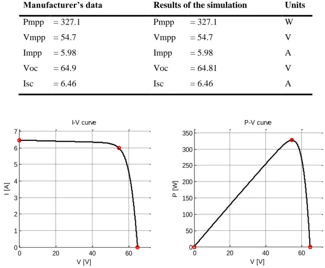
After building a general simulation of PV generator, the simulation is tested with data of photovoltaic module “Sunpower E20/327 SPR-327NE-WHT-D”.

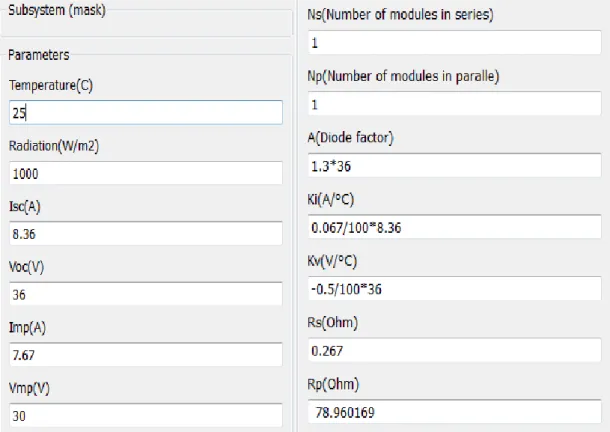
 Data of 1 module “Sunpower E20/327 SPR-327NE-WHT-D”: Pmpp Vmpp Impp Voc Isc Kv Ki = 327 = 54.7 = 5.98 = 64.9 = 6.46 = -176.6 = 3.5 W V A V A mV/°C mA/°C  Model parameters Np Ns A Rs Rp = 1 = 1 = 1.2*96 = 0.2212 = 345.2188 Strings Modules

(Ideal diode factor) Ohm

(22)

Nguyen Ngoc Ban Page 21  Results:

Table 2.2: Comparison of manufacturer’s data with results of the simulation

Manufacturer’s data Results of the simulation Units

Pmpp Vmpp Impp Voc Isc = 327.1 = 54.7 = 5.98 = 64.9 = 6.46 Pmpp Vmpp Impp Voc Isc = 327.1 = 54.7 = 5.98 = 64.81 = 6.46 W V A V A

Figure 2.1: I-V curve of 1 module E20 Figure 2.2: P-V curve of 1 module E20

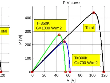
2.1.2. Photovoltaic modules in series

To increase output voltage, PV modules are connected in series. The current through these modules is the same, but the total output voltage is the sum of output voltage across each module. If modules are under the same conditions of solar radiation and temperature, there is nothing special. However, if modules are under different conditions, for example some shaded by trees or clouds, the output current is strongly affected by the current of the shaded PV module, because when the current is higher than short circuit current of shaded module, it produces negative voltage and makes the sum of voltage reduce very fast.

In order to prevent this situation, bypass diodes are used (ASTIER, 2013). When having bypass diode, the total output current is not affected by the shaded PV module. Any negative

0 20 40 60 0 1 2 3 4 5 6 7 I-V curve V [V] I [A ] 0 20 40 60 0 50 100 150 200 250 300 350 P-V curve V [V] P [ W ]

(23)

voltage of shaded PV module is cut by its diode bypass, so the total voltage will follow the output voltage of the not shaded PV module with small difference equal the forward voltage of bypass diode. Besides, in this case the total output power curve will have some peaks (1 global maximum power point and some local maximum power points) and it will make the process of determination of maximum power point become more difficulty.

Hereunder, it is the results of simulation of the PV system including 2 modules E20 in 2 cases: without bypass diode and with bypass diode.

Figure 2.3: I-V curve of 2 modules E20 in series without diode bypass

Figure 2.4: P-V curve of 2 modules E20 in series without diode bypass

When 2 above modules are connected in series with diode bypass, the result is obtained:

Figure 2.5: I-V curve of 2 modules E20 in series with diode bypass

Figure 2.6: P-V curve of 2 modules E20 in series with diode bypass

0 20 40 60 80 100 120 0 1 2 3 4 5 6 7 I-V curve V [V] I [A ] Total T=350K G=1000 W/m2 T=300K G=700 W/m2 0 20 40 60 80 100 120 0 100 200 300 400 P-V curve V [V] P [ W ] Total T=350K G=1000 W/m2 T=300K G=700 W/m2 0 20 40 60 80 100 120 0 1 2 3 4 5 6 7 I-V curve V [V] I [A ] T=350K G=1000 W/m2 T=300K G=700 W/m2 Total 0 20 40 60 80 100 120 0 100 200 300 400 P-V curve V [V] P [ W ] Total T=300K G=700 W/m2 T=350K G=1000 W/m2

(24)

These simulating results are theoretical true when two real PV modules are associated in series. Therefore, the program works well in this situation.

2.1.3. Photovoltaic modules in parallel

To increase output current of a PV system, PV modules are associated in parallel. The voltage at two terminals of these modules is the same, but the total output current is the sum of output current of each module. In case of different voltages of legs, due to shading or temperature difference, one leg can produce negative current in other one which makes the global output current reduce very fast.

In order to prevent this situation, blocking diodes connected in series in each leg are used (ASTIER, 2013). When having blocking diode, the total output voltage is not affected by unbalances. Any negative current in a leg is cut by its blocking diode, so the total current will follow the output current of stronger ones. Besides, in this case the total output power curve will have some peaks (1 global maximum power point and some local maximum power points) and it will make the process of determination of maximum power point become more difficulty.

Figure 2.7: I-V curve of 2 modules E20 in parallel without blocking diode

Figure 2.8: P-V curve of 2 modules E20 in parallel without blocking diode

0 10 20 30 40 50 60 0 2 4 6 8 10 12 I-V curve V [V] I [A ] T=350K G=1000W/m2 T=300K G=700W/m2 Total 0 10 20 30 40 50 60 0 100 200 300 400 500 P-V curve V [V] P [ W ] T=350K G=1000W/m2 T=300K G=700W/m2 Total

(25)

When 2 above modules are connected in parallel with blocking diode, the result is obtained:

Figure 2.9: I-V curve of 2 modules E20 in parallel with blocking diode

Figure 2.10: P-V curve of 2 modules E20 in parallel with blocking diode

Like section “2.1”, this section gives reasonable results in case of connecting with blocking diode.

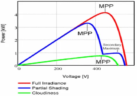
2.2. Maximum power point tracking

The function of maximum power point tracking is to maximize the output power of a PV system at any conditions of temperature and solar radiation. The investment cost of a PV system is quite high and therefore customers always want to get the highest energy produced by this system and thereby minimize the cost and also the Energy Pay Back Time (EPBT). The variation of irradiation and temperature make the maximum power point (MPP) unstable, so it needs appropriate algorithms to track the MPP and keep this value constantly (D.Hohm & M.Ropp, 2003).

In order to get the necessary freedom degree to achieve MPPT, the PV array can be connected with a DC-DC converter with D duty cycle (Buck, Boost, and Buck-Boost) and then supplying the load.

0 20 40 60 0 2 4 6 8 10 12 I-V curve V [V] I [A ] Total T=300K G=700W/m2 T=350K G=1000W/m2 0 20 40 60 0 100 200 300 400 500 P-V curve V [V] P [ W ] Total T=350K G=1000W/m2 T=300K G=700W/m2

(26)

Nguyen Ngoc Ban Page 25 With buck converter:

2 2 . / . / Vo Vin D Pin Po Io Iin D Ro Rin D Rin Ro D         Since 0 D 1 , soRinRo. Where:

 Vin: Input voltage of buck converter (output voltage of the PV array)

 Iin: Input current of buck converter (output current of the PV array)

 Pin: Input power of buck converter (output power of the PV array)

 Vo: Output voltage of buck converter

 Io: Output current of buck converter

 Po: Output power of buck converter

 Ro: Load after buck converter

 Rin: Resistor at working point of PV array

 D: Duty cycle of buck converter

At maximum power point of PV array, we have Ropt.

 If Ropt < Ro => can’t reach Ropt.

 If Ropt > Ro => possibility to reach Ropt, it depends on D.

With boost converter:

Rin=Ro.(1-D)2 <= Ro

 If Ropt > Ro => can’t reach Ropt.

 If Ropt < Ro => possibility to reach Ropt, it depends on D.

With buck-boost converter:

(27)

Nguyen Ngoc Ban Page 26  In this case D can be adjusted to Rin=Ropt

In order to reach MPP of PV array, D have to be adjusted by MPPT.

There are many proposed algorithms but 2 common methods of maximum power point tracking are used popularly:

 Incremental conductance (INC)

 Perturbation and observation (P&O)

In this report, I mention the P&O method because it is simple and used the most in commercial MPPT (D.Hohm & M.Ropp, 2003). Afterward I will present small modification to make it work faster.

Figure 2.11: Maximum power point at different condition

2.2.1. Perturbation and observation

The idea of P&O method is to vary output voltage with small step and to observe the change of output power. If the increasing of the voltage induces the increasing of the power, the voltage is stepped up. Conversely, if the growth of the voltage causes the decreasing of the power, the voltage is stepped down (D.Hohm & M.Ropp, 2003).

(28)

The tracking diagram of P&O method is presented in follow picture:

Figure 2.12: Perturbation and observation method

However, this method will cause the oscillation phenomenon around the maximum power point. The oscillation depends on the step of perturbation of duty cycle of static converter (buck, boost or buck-boost). If the step is very small, the magnitude of the change is very small too, but it takes long time to reach MPP. Besides, if the step is big, the magnitude of the variation is big too, but it takes short time to reach MPP. Therefore, choosing a suitable step is the most important point of P&O method to achieve the desired effect.

(29)

Figure 2.13: Perturbation and observation flow chart

Modification of P&O method

With above model, D starts from 0, then adjusting with ∆D. If ∆D large, MPP is found fast but the working point oscillates quite far from MPP. If ∆D small, MPP is found slower but the working point oscillates very near from MPP.

From this situation, I suggest:

 D starts from 0.5, because D=0.5 the possibility to reach any point of D is faster than D=0

 Using variable step ∆D:

o Using large ∆D at the beginning to reach MPP faster

START READ V(k),I(k) P(k)= V(k),I(k) ∆P=P(k)-P(k-1) ∆V=V(k)-V(k-1) ∆P > 0 ∆V < 0 ∆V < 0 D=D+∆D D=D-∆D D=D-∆D D=D+∆D

(30)

Nguyen Ngoc Ban Page 29 o Using small ∆D later to minimize the oscillation

Compare the results:

The maximum power in following tests is 230.1 W.

Table 2.3: Comparison of the results

Test 1 Test 2 Test 3 Test 4

Ppv (W) ∆D Time at MPP (s) 141.1 Non 0.03 227.5  2.7 0.01 0.06 230.05  0.5 0.001 0.38s 230.05  0.5 Variable 0.07 Commentary:

 With modification of P&O method, the PV system can reach MPP fast and very small oscillation. It takes advantages of large step and small step of ∆D.

2.2.2. Sweeping technique with voltage regulation

In uniform conditions of temperature and irradiation or the variation of this condition is not too fast, the perturbation and observation method works quite well. This algorithm is useful because there is only one max point in such conditions. However, in case of shading onto some modules, the power curve will have one global maximum power point and some local ones and therefore P&O method does not operates efficiently. Using the variation of voltage and observe changing direction of the power, this method will find the first local maximum power point and it is trapped at this point. Hence, the global MPP is not found and the output power of the PV system is not optimal.

In practical, there are some methods such as Fuzzy and Particle Swarm Optimization (Sarvi, Tabatabaee, & Soltani, 2013) to find global MPP in shading condition, but it is complicated. In this report, I would like to introduce a simple and efficient method, called Sweeping Technique associated to a voltage regulation. The idea of this method is measuring all the possibility of power, detecting the maximum power Pmpp and associated voltage Vmpp then used as the reference of a voltage regulated supply as shown on figure 2.14. The advantages are a robust work and the ability of piloting the output power between zero and Pmpp if necessary, for example in the case of a lot of sun and no demand (battery full of charge, …).

(31)

In order to get values of power, the static characteristic of the PV generator is swept during a given short time tsw by varying the duty cycle of static converter (buck converter) from 0 to 1.

By using comparative algorithm, the maximum power point and optimal voltage at any given conditions are then known. Now, by keeping this voltage constant by means of a voltage regulation acting on D, the optimal power is maintained so long that no changing. When there is any changing of temperature or solar radiation occuring, output current of the PV system also changes. If it differs from the previous value of 2%, an algorithm is activated to operate the sweeping process and refresh the new maximum power point and optimal voltage reference. (Appendix D)

(32)

Hereunder, it is the comparison of behavior of P&O method and Sweeping method at condition: T=250C and G=700+300*sin(2*pi*1/1*t) , period = 1s

Figure 2.15: P&O method Figure 2.16: Sweeping method

It can be seen that a better result is obtained by Sweeping Technique. This method detects optimal voltage and maintains it. It is lucky that this voltage suffers very small influence from irradiation. 0 0.5 1 1.5 2 2.5 3 3.5 4 0 50 100 150 200 250 Power curve Time (s) P o w e r (W ) Ideal Power Real Power 0 0.5 1 1.5 0 50 100 150 200 250 Power curve Time (s) P o w e r (W ) Ideal Power Real Power

(33)

CHAPTER III: SIMULATION OF PHOTOVOLTAIC EMULATOR

3.1. Objective

The development of PV industry is getting faster and faster and demand of specialized equipment for testing at a lab such as the LAPLACE is indispensable. However, in order to test the behavior of a real PV system, it requires a large space to install the modules, a big investment cost. Besides, it highly depends on outdoor weather conditions. It is unpredictable and uncontrollable (Piazza & Vitale, 2013) and it does not work at night.

To handle this problem, an alternative solution is considered and PV emulator is the key of this issue. The objective of it is to produce current and voltage characteristic from main grid with the same behavior of a PV system, but PV emulator is electronic equipment, virtual PV modules. It can be placed into a room to test behavior of any PV modules associated with batteries, pumps, current source plus load, voltage source plus load or MPPT plus DC-DC converter and load.

PV emulator can work independently without constraint of outside weather condition, it is cheaper than a real PV array and particularly it can test many type of PV modules by changing input data on software. This cannot be done by a real one.

3.2. Structure of a photovoltaic emulator

Different structures can be used to realize a PV emulator. We choose one based on the presented developed PV model which drives a DC-DC converter owing to a Hardware in the Loop (HIL) structure. This Photovoltaic emulator is composed of 4 main parts:

 A simulation of photovoltaic module (PV model)

 A DC-DC converter (Buck converter)

 A real power source (supply from main grid)

(34)

Figure 3.1: Principle and structure HIL of the PV emulator

Working principle of a PV emulator:

 Supply a real direct source such as voltage is 500V to static converter.

 Measure output current of the PV emulator (Ip), this is the value of output current of static converter to the actual load.

 Simulation with the PV model provides the value of output voltage Vp at given condition of temperature, irradiation and information of tested PV module corresponding to actual Ip.

 Control system controls the duty cycle of static converter so that output voltage of this converter equal Vp (Ip).

3.3. Photovoltaic emulator in SIMULINK

Before making a real PV emulator, it is useful to simulate this emulator on MATLAB SIMULINK in order to know its behavior and from the results it can be concluded that the PV emulator will work well or inefficiently.

In this report, simulation of PV emulator is tested with data of PV module “Sunpower

E20/327 SPR-327NE-WHT-D” and three kinds of load:

 Current source associated with resistance in parallel (Case 1)

 Voltage source associated with resistance in series (Case 2)

(35)

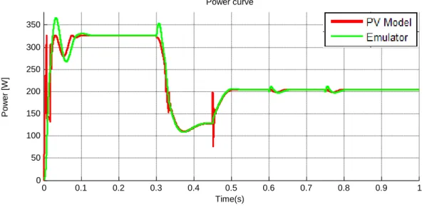
Figure 3.2: Power curve of PV model and emulator in case 1

Figure 3.3: Power curve of PV model and emulator in case 2

Based on general structure of PV emulator in section “3.2”, structures of emulator with load in case 1, case 2 and case 3 are presented in appendix E. From these, power curves of PV model and emulator in case 1 and case 2 are obtained and showed in figure 3.2 and figure 3.3. It can be seen that characteristic of output voltage and output power of simulation of emulator are the same with the characteristic of PV module “Sunpower E20/327 SPR-327NE-WHT-D” in two first cases.

In case 3, structure in MATLAB SIMULINK is more complex than case 1 and case 2. To make it easy, buck converter in PV emulator and on the load side named converter 1 and converter 2 respectively. 0 10 20 30 40 50 60 70 0 50 100 150 200 250 300 350 Power curve Voltage (V) P o w e r [W ] PV model Emulator 0 20 40 60 50 100 150 200 250 300 350 Power curve Voltage (V) P o w e r (W ) PV model Emulator

(36)

Figure 3.4: Structure of photovoltaic emulator in case 3

Measurement of output current of PV emulator is different from two previous cases because in this case switching function of IGBT in converter 2 makes a large oscillation of the current. This variation makes the control system in the emulator cannot regulate output voltage of converter 1 to be the same with output voltage of PV model.

In order to solve this problem, low pass filter is required to get average value of the current. There are two kinds of this filter: analog low pass filter and physical low pass filter. Using analog filter is better because it is a software function while physical filter is composed of one inductor and one resistor, less flexible and introducing more devices and losses in the system. In figure 3.4, there is a capacitor C between converter 1 and converter 2. The value of this capacitor will affect the oscillation of output power of emulator, so choosing a suitable value is very important: the right value has been found by testing.

(37)

Figure 3.5: Power curve of PV emulator with analog low pass filter (C = 2.2e-3F)

Figure 3.6: Power curve of PV emulator with analog low pass filter (C = 4e-3F)

In case 3, in order to find the maximum power point, MPPT is modified to be able to work well with converter 1 and converter 2. Besides, there are two PV models, one for finding output voltage correspond to measured output current, one for MPPT. After MPPT gives the optimal values of power and voltage of PV module, optimal value of duty cycle of converter 2 can be known and then converter 2 is controlled by this duty cycle. Using sweeping technique directly for converter 2 is not efficient because the interaction of converter 1 and converter 2 make it very difficult.

At steady state conditions of temperature and irradiation, the results of simulation of PV emulator is very good, but there are small difference between output of PV emulator and PV model during transients, a property to be improved in a future work if necessary.

0 0.1 0.2 0.3 0.4 0.5 0.6 0.7 0.8 0.9 1 0 50 100 150 200 250 300 350 Power curve Time(s) P o w e r [W ] 0 0.1 0.2 0.3 0.4 0.5 0.6 0.7 0.8 0.9 1 0 50 100 150 200 250 300 350 Power curve Time(s) P o w e r [W ]

(38)

Nguyen Ngoc Ban Page 37 CONCLUSION

This work proposed a quite good modeling and simulation of photovoltaic generator in MATLAB SIMULINK. Values of short circuit current, open circuit voltage, current and voltage at maximum power at standard test conditions are almost the same with manufacturers’ data and the model is usable a differents scales : PV cell, PV module, PV array. Models of cells or modules can be connected together so as to simulate associations. Moreover, the obtained characteristic of output current vs output voltage when PV modules are connected in series with bypass diode and in parallel with blocking diode are in right agreement with theory and practice.

A classic maximum power point tracking method, perturbation and observation, is also presented. This method can work quite well under conditions of slow variation of temperature and irradiation and without shading by clouds, buildings or trees. However, in case of shading condition, having several maximum points makes P&O method work inefficiently. In this situation, an original sweeping technique has been proposed to identify global maximum power point Pmpp and associated voltage Vmpp, though there are some local peaks. The MPPT is then realised by means of regulating of the PV string output voltage to Vmpp, which is better for efficiency and robust. Moreover, it enables to deactivate MPPT function in order to control the actual output power betwen Pmax and Zero, by choosing the voltage reference different from Vmpp. This function is useful in smart-grids when reducing power generation is required.

Finally, a PV emulator based on the previous PV model has been proposed and its simulation achieved. The results simulation of photovoltaic emulator have demonstrated a right work to behave as an actual PV module or large array without investing an expensive practical one. However, it still requires more study to improve the stability and acuracy on transcients..

(39)

REFERENCES

ASTIER, S. (2013). Photovoltaic Solar System.

D.Hohm, & M.Ropp. (2003). Comparative Study of Maximum Power Point Tracking Algorithms. Electrical Engineering Department, South Dakota State University,

Brookings, SD 5700-2220, USA, 1.

http://www.pveducation.org/pvcdrom.

J.Nicolas. (2013). Renewable Energy and Demand Side Management.

M.Villalva, R.Jonas, & R.Ernesto. (2009). Comprehensive Approach to Modeling and Simulatino of Photovoltaic Arrays. IEEE Transactions on Power Electronics, 24(5), 1-2.

Mathworks. (2014). Simulink® Getting Started Guide.

Piazza, M. C. D., & Vitale, G. (2013). Photovoltaic Sources Modeling and Emulation. London: Springer.

Said, S., Massoud, A., Benammar, M., & Ahmed, S. (2012). A Matlab/Simulink-Based Photovoltaic Array Model Employing SimPowerSystems Toolbox. Energy and Power

Engineering, 4.

Sarvi, M., Tabatabaee, M. H., & Soltani, I. (2013). A Fast Maximum Power Point Tracking for mismatching compensation for PV Systems under Normal and Partially Shaded Conditions. Journal of mathematics and computer science.

(40)

Nguyen Ngoc Ban Page 39 APPENDIX A

STRUCTURE OF PV STRINGS AT ENSEEIHT AND LABEGE

(41)

(42)

Nguyen Ngoc Ban Page 41 APPENDIX B

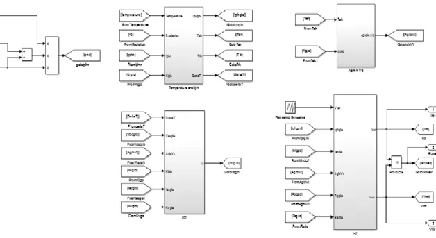
STRUCTURE OF PHOTOVOLTAIC MODULE IN MATLAB SIMULINK

Figure B.1: Simulation of PV module in MATLAB SIMULINK

(43)

Figure B.3: Structure under PV module

(44)

Figure B.5: Subsystem 1 to obtain temperature and Iph

(45)

Figure B.7: Structure under subsystem oC to Kelvin

(46)

Figure B.9: Structure under subsystem 2

(47)

(48)

Iterative algorithm code to find Rs and Rsh of Sunpower E20/327 SPR-327NE-WHT-D:

%% Information from the solar array datasheet

Iscn = 6.46; %Nominal short-circuit voltage [A]

Vocn = 64.9; %Nominal open-circuit voltage [V]

Imp = 5.98; %Current at maximum power point [A]

Vmp = 54.7; %Voltage at maximum power point [V]

Pmax_e = Vmp*Imp; %Maximum output peak power [W]

Kv = -176.6*10^-3; %Temperature coefficient of voltage [V/K]

Ki = 3.5*10^-3; %Temperature coefficient of current [A/K]

Ns = 96; %Number of series cells

a = 1.2; %Ideality diode factor

%% Program inputs

Gn = 1000; %Nominal irradiance [W/m^2] @ 25°C

Tn = 25 + 273.15; %Nominal operating temperature [K]

%% Algorithm parameters %Increment of Rs

(49)

Nguyen Ngoc Ban Page 48 %Maximum tolerable power error

tol = 0.0001; %Defines the model precision %Voltage points in each iteraction

nv = 5000; %Defines how many points are used for obtaining the IxV curve

nimax = 500000; %Avoids program stall in case of non convergence %% Adjusting algorithm

% Reference values of and Rp

Rp_min = Vmp/(Iscn-Imp);

% Initial guesses of Rp and Rs

Rs = 0;

Rp = Rp_min;

% The model is adjusted at the nominal condition

T = Tn; dT = T-Tn; G = Gn;

k = 1.3806503e-23; %Boltzmann [J/K]

q = 1.60217646e-19; %Electron charge [C]

Vtn = k * Tn / q; %Thermal junction voltage (nominal)

Vt = k * T / q; %Thermal junction voltage (current temperature)

perror = Inf; %dummy value(help to run program at the beginning)

% Iterative process for Rs and Rp until Pmax,model = Pmax,experimental

ni = 0;

while (perror>tol) && (Rp > 0) && (ni < nimax)

ni = ni + 1;

Ipvn = (Rs+Rp)/Rp * Iscn; % Nominal light-generated current

Ipv = (Ipvn + Ki*dT) *G/Gn; % Actual light-generated current

Isc = (Iscn + Ki*dT) *G/Gn; % Actual short-circuit current

Io = (Iscn + Ki*dT)/(exp((Vocn+Kv*dT)/(Vt*a*Ns))-1); % consider a panel as one cell

% Increments Rs Rs = Rs + Rsinc; Rp_ = Rp; Rp = Vmp*(Vmp+Imp*Rs)/(Vmp*Ipv-Vmp*Io*exp((Vmp+Imp*Rs)/(Vt*Ns*a))+Vmp*Io-Pmax_e); V = 0:Vocn/nv:Vocn; % Voltage vector

I = zeros(1,size(V,2)); % Current vector, with intial value=0

for j = 1 : size(V,2) %Calculates for all voltage values

% Solves g = I - f(I,V) = 0 with Newton-Raphson

g(j) = Ipv-Io*(exp((V(j)+I(j)*Rs)/(Vt*Ns*a))-1)-(V(j)+I(j)*Rs)/Rp-I(j); while (abs(g(j)) > 0.001)

g(j) = Ipv-Io*(exp((V(j)+I(j)*Rs)/(Vt*Ns*a))-1)-(V(j)+I(j)*Rs)/Rp-I(j); glin(j) = -Io*Rs/Vt/Ns/a*exp((V(j)+I(j)*Rs)/Vt/Ns/a)-Rs/Rp-1; % derivative g(j)

I_(j) = I(j) - g(j)/glin(j); I(j) = I_(j);

(50)

Nguyen Ngoc Ban Page 49 end P = (Ipv-Io*(exp((V+I.*Rs)/(Vt*a*Ns))-1)-(V+I.*Rs)/Rp).*V; Pmax_m = max(P); perror = (Pmax_m-Pmax_e); end

disp(sprintf('Model info:\n')); disp(sprintf(' Rp = %f',Rp)); disp(sprintf(' Rs = %f',Rs)); disp(sprintf(' a = %f',a));

disp(sprintf(' T = %f',T-273.15)); disp(sprintf(' G = %f',G));

disp(sprintf(' Pmax,m = %f (model)',Pmax_m)); disp(sprintf(' Pmax,e = %f (experimental)',Pmax_e)); disp(sprintf(' tol = %f',tol));

disp(sprintf('P_error = %f',perror)); disp(sprintf(' Ipv = %f',Ipv)); disp(sprintf(' Isc = %f',Isc)); disp(sprintf(' Io = %g',Io)); disp(sprintf('\n\n'));

(51)

Nguyen Ngoc Ban Page 50 APPENDIX C

DATA SHEET OF SITE ENSEEIHT AND SITE LABEGE

1. Site ENSEEIHT 1.1. Section PV_N1

Section N1 is composed 24 photovoltaic modules “Sunpower E20/327 SPR-327NE-WHT-D”. The electrical coupling of the 24 modules is made of 4 strings of 6 modules.

 Data of 1 module “Sunpower E20/327 SPR-327NE-WHT-D”: Pmpp Vmpp Impp Voc Isc Kv Ki = 327 = 54.7 = 5.98 = 64.9 = 6.46 = -176.6 = 3.5 W V A V A mV/°C mA/°C  Model parameters Np Ns A Rs Rp = 4 = 6 = 1.2*96 = 0.2212 = 345.2188 Strings Modules

(52)

Hereunder, it is the results of simulation of PV_N1 under 2 conditions “Standard Test Condition (STC)” and “Practical Test Condition (PTC)”:

 Standard Test Condition (T=25°C, G=1000W/m2)

Vmpp Impp Pmpp = 328.260 = 23.915 = 7850.546 (V) (A) (W)

Figure 1.1: I-V curve of PV_N1 at STC

 Practical Test Condition (T=50°C, G=800W/m2)

Figure 1.2: I-V curve of PV_N1 at PTC

0 50 100 150 200 250 300 350 400 0 5 10 15 20 25 I-V curve V [V] I [A ] 0 50 100 150 200 250 300 350 0 5 10 15 20 I-V curve V [V] I [A ]

(53)

Nguyen Ngoc Ban Page 52 1.2. Section PV_N2

Section N2 is composed 9 photovoltaic modules “Panasonic-Sanyo VBHN240SE10”. The electrical coupling of the 9 modules is made of 1 string of 9 modules.

 Data of 1 module “Panasonic-Sanyo VBHN240SE10”: Pmpp Vmpp Impp Voc Isc Kv Ki = 240 = 43.7 = 5.51 = 52.4 = 5.85 = -131 = 1.76 W V A V A mV/°C mA/°C  Model parameters Np Ns A Rs Rp = 1 = 9 = 1.5*72 = 0.3001 = 1575.6850 Strings Modules

(54)

0 100 200 300 400 500 0 1 2 3 4 5 6 I-V curve V [V] I [A ] 0 100 200 300 400 0 1 2 3 4 5 I-V curve V [V] I [A ]

(55)

Section N3 is composed 18 photovoltaic modules “First Solar FS390”. The electrical coupling of the 18 modules is made of 2 strings of 9 modules.

 Data of 1 module “First Solar FS390”: Pmpp Vmpp Impp Voc Isc Kv Ki = 90 = 47.4 = 1.9 = 60.5 = 2.06 = -0.27%*Voc = 0.04%*Isc W V A V A V/°C A/°C  Model parameters Np Ns A Rs Rp = 2 = 9 = 1.5*90 = 2.1158 = 4850.469366 Strings Modules

(56)

0 100 200 300 400 500 0 1 2 3 4 I-V curve V [V] I [A ] 0 100 200 300 400 500 0 0.5 1 1.5 2 2.5 3 3.5 I-V curve V [V] I [A ]

(57)

Section N4 is composed 16 photovoltaic modules “Avancis PowerMax Strong 125Wc”. The electrical coupling of the 16 modules is made of 2 strings of 8 modules.

 Data of 1 module “Avancis PowerMax Strong 125Wc”: Pmpp Vmpp Impp Voc Isc Kv Ki = 125 = 43.8 = 2.85 = 59.1 = 3.24 = -170 = 0.1 W V A V A mV/°C mA/°C  Model parameters Np Ns A Rs Rp = 2 = 8 = 1.5*72 = 2.6839 = 231.878986 Strings Modules

(58)

0 100 200 300 400 500 0 1 2 3 4 5 6 7 I-V curve V [V] I [A ] 0 100 200 300 400 0 1 2 3 4 5 I-V curve V [V] I [A ]

(59)

Nguyen Ngoc Ban Page 58 2. Site LABEGE

2.1. Section PV_I1

Section I1 is composed 24 photovoltaic modules “Sunpower E20/327 SPR-327NE-WHT-D”. The electrical coupling of the 24 modules is made of 4 strings of 6 modules.

(60)

Hereunder, it is the results of simulation of PV_I1 under 2 conditions “Standard Test Condition (STC)” and “Practical Test Condition (PTC)”:

Figure 2.1: I-V curve of PV_I1 at STC

Figure 2.2: I-V curve of PV_I1 at PTC

0 50 100 150 200 250 300 350 400 0 5 10 15 20 25 I-V curve V [V] I [A ] 0 50 100 150 200 250 300 350 0 5 10 15 20 I-V curve V [V] I [A ]

(61)

Nguyen Ngoc Ban Page 60 2.2. Section PV_I2

Section I2 is composed 24 photovoltaic modules “Panasonic-Sanyo VBHN240SE10”. The electrical coupling of the 24 modules is made of 3 strings of 8 modules.

 Data of 1 module “Panasonic-Sanyo VBHN240SE10”: Pmpp Vmpp Impp Voc Isc Kv Ki = 240 = 43.7 = 5.51 = 52.4 = 5.85 = -131 = 1.76 W V A V A mV/°C mA/°C  Model parameters Np Ns A Rs Rp = 3 = 8 = 1.5*72 = 0.3001 = 1575.685063 Strings Modules

(62)

Hereunder, it is the results of simulation of PV_I2 under 2 conditions “Standard Test Condition (STC)” and “Practical Test Condition (PTC)”:

Figure 2.3: I-V curve of PV_I2 at STC

Figure 2.4: I-V curve of PV_I2 at PTC

0 100 200 300 400 0 5 10 15 I-V curve V [V] I [A ] 0 50 100 150 200 250 300 350 400 0 5 10 15 I-V curve V [V] I [A ]

(63)

Nguyen Ngoc Ban Page 62 2.3. Section PV_I3

Section I3 is composed 18 photovoltaic modules “Sunpower E20/327 SPR-327NE-WHT-D”. The electrical coupling of the 18 modules is made of 2 strings of 9 modules.