THÈSE
En vue de l’obtention du
DOCTORAT DE L’UNIVERSITÉ DE TOULOUSE
Délivré par l'Université Toulouse 3 - Paul Sabatier
Présentée et soutenue par
Yseult HEJJA--BRICHARD
Le 10 juin 2020
Spatial and temporal integration of binocular disparity in the
primate brain
Ecole doctorale : CLESCO - Comportement, Langage, Education, Socialisation, Cognition
Spécialité : Neurosciences, comportement et cognition Unité de recherche :
CERCO - Centre de Recherche Cerveau et Cognition Thèse dirigée par
Benoit COTTEREAU Jury
M. Peter JANSSEN, Rapporteur Mme Claire WARDAK, Rapporteure
Mme Kristine KRUG, Examinatrice M. Jean-Marc DEVAUD, Examinateur M. Benoit R. COTTEREAU, Directeur de thèse
SPATIAL AND TEMPORAL INTEGRATION OF
BINOCULAR DISPARITY IN THE PRIMATE BRAIN
i
Acknowledgements
Before anything, I would like to express my sincere gratitude to the members of my thesis committee: Prof. Peter Janssen, Dr. Claire Wardak, and Prof. Kristine Krug who, despite the postponing of my defence by seven long months have nonetheless accepted to examine and review my work; and Prof. Jean-Marc Devaud who kindly accepted to join the final version of it and is also symbolically closing a loop, as I arrived in Toulouse to enrol in the master’s degree he was co-directing.
I would like to say how grateful I am to Benoit, who supervised me as a master’s student and then as his first PhD student. Thank you for trusting me and giving me the right amount of autonomy whilst being always available, for letting me go at my own pace, and for your guidance throughout my PhD studies. Thank you for being so optimistic when I was rather sceptical or a bit demotivated, for pushing me when I needed it, for providing me with the right framework to express my doubts, my hesitations, but also to encourage me to develop my own ideas.
I had a great time at the lab and felt very supported by the Eco-3D team. I am truly grateful for the openness, the kindness, and the support of all of its members and for whom I would like to have a word:
Jean-Baptiste for his priceless help with the analyses, his advice, his availability Youn for his extensive knowledge of the literature, for his listening
Alexandra for introducing to me the teaching side of academia.
Tushar for the endless conversations we had, for dealing with me and my many questions, for your creativity regarding new experiment ideas, for your enthusiasm
Silvia who I was happy to work with and who helped me a lot for running the human experiments when I had to focus on writing my thesis!
Vanessa who joined the team more lately with her energy and dedication!
Pauline who has picked up the torch to further help develop monkey fMRI in the team. It was also quite pleasant to see more women joining the team!
I am also thinking of former PhD students and post-docs. Special thanks to Samy who set the path to my PhD and took time to guide me through the different steps, for the many philosophical discussions. Marcello and Volodymyr with whom I shared the office, and for the many debates and discussions that took place in that office; Amirouche as well. Mylène and Emilie who I started this adventure with.
ii Thank you to my closest toulousain friends and lab mates, Chadlia and Nicolas, with whom I shared my frustrations, my joy, my reliefs; for putting up with me at every moment.
Thank you Manu, Petit Pascal, Jean-Michel for the discussions we had about how to change the world, for sometimes turning words into actions; the PAF students: Sam, Can, Bhavin, Zhaoyang, Milad, Benjamin for the restaurant sessions, and the organisation of events within and outside the lab; to the second floor students, present despite geographical constraints, especially to Mariam, Danaé, Ludovic, and for their involvement in the lab life (which really matters to me, as some may have noticed!), Anna with whom I shared some teaching stress. Thank you, Marine who I started my journey in Toulouse with, balancing between heavy fun and light seriousness! To our long phone calls across the country and now the ocean!
Thank you, Emilie Rapha for your priceless help and your everyday investment, Camille Lejards for teaching me in the first place how to work with macaques and for believing I could talk with them.
Obviously, I now have to mention Nikita and Tunisie, my two monkey mates, who I worked with during those 5 years. That was not an easy task but it was clearly worth it!
I would like to thank the MRI facility staff, Nathalie, but also Hélène and the ‘manip radio’ team, Jean-Pierre, Yohan, and Fred.
But also, the several persons in charge of less obvious aspects of research, the IT team for both their technical and moral support: Carmen, Maxime, Damien, Joel; and Claire for dealing with all the financial and some administrative aspects of research.
I also want to thank all the other CerCo members, former and current, that I did not mention but who clearly played a big role into making this place a vibrant place for doing a PhD and for growing up as a future – and hopefully good – researcher. And Simon for giving so much freedom to the students as the director of the lab; this is very valuable and rewarding!
I would like to thank the teaching team of the 'section 69' for welcoming me as a teaching assistant during my first three years.
Merci à InCOGnu and its enthusiastic members who I got to spend time with: Nabila, Lucille, Laura, Joseph, Nawelle, Simon, Mehdi, Alice, Bonnie, Audric, Maxime, Mawa, Amélie, Quentin, Lisa. I had fun during our science popularisation events, it brought me a lot and helped me figure out this is something that really matters to me.
iii I also want to mention the different persons who paved the way that led me to do this PhD: Natacha Mendès who took me as a trainee research assistant on her postdoc project seven years ago and introduced me to the wonderful world of working with non-human primates; Eugénie Lhommée with whom I did my first clinical internship and who supported me when I chose to study fundamental research instead of clinical neuropsychology; Olivier Pascalis who offered me my first research internship.
A big thought goes to Slowpen who gave me hope into a more human science framework, Amélie, Brice, Lad, and Bertrand, for those countless discussions we had, for those weekends and skype meetings we spent together thinking about how to improve science practices, for teaching me Bayesian philosophy, and for so many other valuable things. I truly value those moments and my friendship with you!
Thanks to my old friends Laureline and Fabien. Even though we don’t meet often (and not often enough), you bring me lots and keep me rooted in the ‘outside world’.
Endlich, bin ich in Gedanken bei meiner liebe leipzigerinnen Freundinnen: Clo, Moira, Sophie, Anna und Sam!
Thank you to my coolest-roommates-ever, Laura and Valentine, with whom I spent lots of time discussing about how to start a world revolution but who also had to put up with my fluctuating mood. A big hug to Babou the ‘cat king’ as well. You were like my second family, which means a lot to me!
Thank you to my close family members, and especially my mother, always very proud and supportive, my grandma who makes me constantly look further, and my 'little' brother who finally found his way to do what he always wanted to.
I will close this section by expressing all my gratitude and my heart feelings to the person I am happily walking by every single day, who brings me into a quiet mindset from where I can enjoy the soothing sound of the ebbing tide and the opaque sun light. There is no annoying wind with you, Andrea.
v
Abstract
The primate visual system strongly relies on the small differences between the two retinal projections to perceive depth. However, it is not fully understood how those binocular disparities are computed and integrated by the nervous system. On the one hand, single-unit recordings in macaque give access to neuronal encoding of disparity at a very local level. On the other hand, functional neuroimaging (fMRI) studies in human shed light on the cortical networks involved in disparity processing at a macroscopic level but with a different species. In this thesis, we propose to use an fMRI approach in macaque to bridge the gap between single-unit and fMRI recordings conducted in the non-human and human primate brain, respectively, by allowing direct comparisons between the two species. More specifically, we focused on the temporal and spatial processing of binocular disparities at the cortical but also at the perceptual level. Investigating cortical activity in response to motion-in-depth, we could show for the first time that 1) there is a dedicated network in macaque that comprises areas beyond the MT cluster and its surroundings and that 2) there are homologies with the human network involved in processing very similar stimuli. In a second study, we tried to establish a link between perceptual biases that reflect statistical regularities in the three-dimensional visual environment and cortical activity, by investigating whether such biases exist and can be related to specific responses at a macroscopic level. We found stronger activity for the stimulus reflecting natural statistics in one subject, demonstrating a potential influence of spatial regularities on the cortical activity. Further work is needed to firmly conclude about such a link. Nonetheless, we robustly confirmed the existence of a vast cortical network responding to correlated disparities in the macaque brain. Finally, we could measure for the first time retinal corresponding points on the vertical meridian of a macaque subject performing a behavioural task (forced-choice procedure) and compare it to the data we also collected in several human observers with the very same protocol. In the discussion sections, we showed how these findings open the door to varied perspectives.
Keywords: fMRI – stereopsis – motion-in-depth – slant perception – horopter – non-human primate
vi
Résumé
Le système visuel du primate s’appuie sur les légères différences entre les deux projections rétiniennes pour percevoir la profondeur. Cependant, on ne sait pas exactement comment ces disparités binoculaires sont traitées et intégrées par le système nerveux. D’un côté, des enregistrements unitaires chez le macaque permettent d’avoir accès au codage neuronal de la disparité à un niveau local. De l’autre côté, la neuroimagerie fonctionnelle (IRMf) chez l’humain met en lumière les réseaux corticaux impliqués dans le traitement de la disparité à un niveau macroscopique mais chez une espèce différente. Dans le cadre de cette thèse, nous proposons d’utiliser la technique de l’IRMf chez le macaque pour permettre de faire le lien entre les enregistrements unitaires chez le macaque et les enregistrements IRMf chez l’humain. Cela, afin de pouvoir faire des comparaisons directes entre les deux espèces. Plus spécifiquement, nous nous sommes intéressés au traitement spatial et temporal des disparités binoculaires au niveau cortical mais aussi au niveau perceptif. En étudiant l’activité corticale en réponse au mouvement tridimensionnel (3D), nous avons pu montrer pour la première fois 1) qu’il existe un réseau dédié chez le macaque qui contient des aires allant au-delà du cluster MT et des aires environnantes et 2) qu’il y a des homologies ave le réseau trouvé chez l’humain en réponse à des stimuli similaires. Dans une deuxième étude, nous avons tenté d’établir un lien entre les biais perceptifs qui reflètent les régularités statistiques 3D ans l’environnement visuel et l’activité corticale. Nous nous sommes demandés si de tels biais existent et peuvent être reliés à des réponses spécifiques au niveau macroscopique. Nous avons trouvé de plus fortes activations pour le stimulus reflétant les statistiques naturelles chez un sujet, démontrant ainsi une possible influence des régularités spatiales sur l’activité corticale. Des analyses supplémentaires sont cependant nécessaires pour conclure de façon définitive. Néanmoins, nous avons pu confirmer de façon robuste l’existence d’un vaste réseau cortical répondant aux disparités corrélées chez le macaque. Pour finir, nous avons pu mesurer pour la première fois les points rétiniens correspondants au niveau du méridien vertical chez un sujet macaque qui réalisait une tâche comportementale (procédure à choix forcé). Nous avons pu comparer les résultats obtenus avec des données également collectées chez des participants humains avec le même protocole. Dans les différentes sections de discussion, nous montrons comment nos différents résultats ouvrent la voie à de nouvelles perspectives.
Mots-clés : IRMf – stéréopsie – mouvement 3D – perception des orientations – horoptère – primates non humains
vii
Résumé substantiel en langue française
Présente chez de nombreuses espèces animales, la vision stéréoscopique, ou vision tridimensionnelle, repose sur l'intégration par le système nerveux des différences entre les projections rétiniennes bidimensionnelles d'une scène visuelle. Ces disparités binoculaires, liées au décalage entre nos deux yeux, nous renseignent de façon très précise sur les distances et les profondeurs des éléments constituant une scène visuelle. Avoir accès à ce type d’informations nous permet notamment de localiser et manipuler des objets et donc d’interagir avec notre environnement. Malgré son importance, tous les mécanismes sous-tendant l'extraction et le traitement de l'information tridimensionnelle par notre système visuel ne sont pas bien compris. Les connaissances parcellaires que nous en avons proviennent principalement de l’étude des réponses neuronales à la disparité binoculaire enregistrées dans les aires visuelles de bas niveau et intermédiaires chez le macaque, espèce traditionnellement utilisée comme modèle du système visuel humain. Plus récemment, avec l’avènement des techniques de neuroimagerie, les réseaux impliqués dans le traitement des disparités ont également pu être étudiés chez l’humain. Néanmoins, du fait de la différence de technique d’enregistrement, unitaire d’une part, et macroscopique de l’autre, il reste compliqué de faire des comparaisons inter-espèces. Durant ma thèse, j’ai étudié l’intégration temporelle et spatiale de la disparité binoculaire à un niveau cortical et à un niveau perceptif chez le macaque ainsi que, de façon plus limitée, chez l’humain, en proposant une approche expérimentale qui permette de pallier au besoin d’établir les homologies et différences qu’il pourrait y avoir entre le macaque et l’humain.
Dans un premier chapitre théorique, je propose une introduction générale sur le système visuel qui inclue une explication détaillée du chemin parcouru par un photon de lumière
viii lorsqu’il entre en contact avec la rétine. Je décris ensuite l’anatomie de l’œil ainsi que les différentes cellules qui composent les voies visuelles avant l’entrée de l’information dans le centre nerveux central, je passe également en revue la phototransduction, phénomène qui permet de transposer le signal électromagnétique du photon à un signal membranaire interprétable par les cellules du système visuel. Je détaille ensuite les deux voies visuelles traditionnellement décrites : la voie magnocellulaire, aussi appelée voie du mouvement ou voie du ‘où’ et plutôt impliquée dans la vision grossière de par les cellules à grands champs récepteurs qui la composent ; et la voie parvocellulaire, voie des objets, ou voie du ‘quoi’, constituée d’une multitude de cellules à petits champ récepteur, offrant une vision plus détaillée de la scène visuelle. Je clos ce premier chapitre en introduisant la notion de stéréopsie, ou vision de la profondeur, présente chez de nombreuses espèces du règne animal, et qui constitue le cœur de mes travaux de thèse.
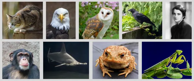
Le chapitre deux, également théorique, offre une revue de la littérature sur l’intégration des disparités binoculaires par le système visuel du primate, en s’appuyant notamment sur des travaux réalisés chez le macaque. Les disparités binoculaires sont un indice de profondeur et de distance utilisées par le système visuel pour extraire l’information tridimensionnelle d’une scène visuelle. Bien qu’il existe de nombreux autres indices, principalement monoculaires (perspectives, ombrages, textures, etc.), les disparités binoculaires permettent au système visuel d’avoir une estimation fine de la structure tridimensionnelle et sous-tendent, au moins chez les primates mais aussi chez d’autres espèces comme le corbeau de Nouvelle Calédonie, l’exécution et le contrôle de gestes précis tels qu’attraper ou manipuler des objets. L’intégration puis le traitement de ces disparités binoculaires auxquelles répondent une multitude d’aires cérébrales représente néanmoins un challenge pour le système visuel de par la nécessité de mettre en correspondance les projections d’une scène visuelle sur chaque
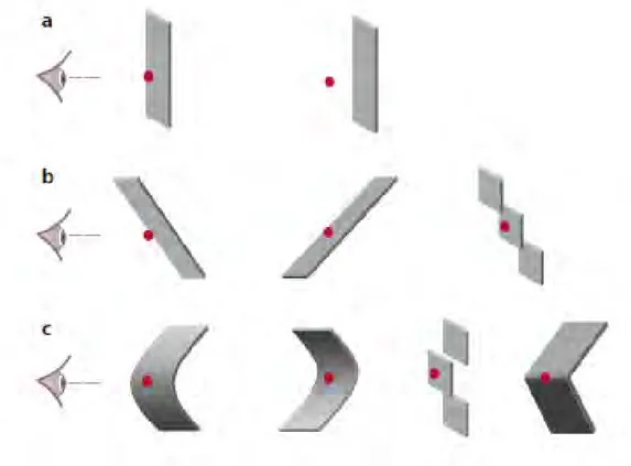
ix rétine. En effet, il n’est pas du tout évident de trouver l’endroit au niveau de chaque rétine sur lequel se projette un point de l’espace visuel. Plusieurs modèles informatiques ont été proposés pour comprendre comment le système visuel résout ce problème de correspondance binoculaire. Parmi eux, le modèle binoculaire d’énergie, développé par Ohzawa et collaborateurs (1990) et évoqué dans ce deuxième chapitre, propose que les neurones complexes de l’aire visuelle primaire (V1) intègrent l’information apportée par des cellules binoculaires simples arrangées en paires de neurones mutuellement inhibitrices. Cette organisation hiérarchique qui repose sur une addition des différentes réponses émises par plusieurs cellules simples offre une solution, parmi d’autres potentielles, au problème de correspondance et suggère que les cellules complexes agissent comme des détecteurs de corrélation entre les deux projections rétiniennes. Ce modèle contient des limitations qui ne permettent pas de le généraliser à toutes les conditions visuelles testées ni aux aires visuelles située au-delà de l’aire V1. Par exemple, les réponses du système visuelle à des points anti-corrélés, points correspondants dans chaque rétine mais à la polarité inversée et qui ne donnent pas de percept 3D, ne sont pas bien prédites par le modèle. Néanmoins, il a le mérite de fournir un cadre de travail intéressant et dont les hypothèses peuvent être testées et affinées. À la suite de la présentation de ce modèle, je précise qu’il existe trois niveaux d’ordre des disparités binoculaires et que ces différents niveaux de profondeur ne sont pas traités de façon identique ni par les mêmes aires visuelles. Concrètement, les disparités binoculaires peuvent être arrangées spatialement de différentes façons et tantôt représenter une simple surface parallèle au plan de fixation, configuration qui correspond à un niveau de profondeur d’ordre zéro, tantôt être organisées sous forme de gradients et prendre la forme de surface orientées ou inclinées (rencontrées dans les scènes visuelles), configuration de premier ordre, qui peuvent contenir des courbures ou des irrégularités dans la surface (c’est le cas pour les objets qui nous entourent) devenant alors de second ordre. Plusieurs travaux de
x neuroimagerie (IRM fonctionnelle) réalisés à la fois chez l’humain et chez le macaque ont pu montrer que plus l’organisation des disparités est complexe et plus les aires cérébrales qui seront actives pour ces arrangements de disparités sont avancées dans la hiérarchie du système visuel. Il y a ainsi une spécialisation de certaines aires cérébrales, qui se développe au fur et à mesure que l’on monte en complexité et qui suit une certaine forme de hiérarchie du système visuel.
Partant ensuite du constat que l’intégration spatiale des disparités binoculaires par le système visuel a été relativement bien documentée chez le primate, j’argumente qu’il y a d’autres questions, complémentaires, qu’il est intéressant de se poser mais qui ont reçu moins d’attention. C’est le cas notamment de l’influence des statistiques naturelles sur le traitement et la perception de ces différentes configurations de disparités. Dans le cadre de ma thèse, je propose d’étudier la façon dont la fréquence d’apparition de différentes orientations et inclinaisons dans les scènes visuelles (premier ordre de profondeur) peut potentiellement impacter leur traitement par le système visuel. En d’autres termes, pourrait-il y avoir une différence au sein des aires cérébrales habituellement impliquées dans le traitement visuel de ces surfaces selon leur fréquence dans les scènes naturelles ? Je suggère également d’étendre cette question à la perception visuelle en étudiant l’influence de ces statistiques naturelles sur la mise en correspondance binoculaire de stimuli tridimensionnels simples.
Enfin, je mets en avant une dimension primordiale dans l’intégration corticale des disparités binoculaires et qui n’a été que trop peu abordée dans la littérature : sa dimension temporelle. En effet, si la vision tridimensionnelle est utilisée pour la manipulation d’objets, elle est aussi extrêmement utile pour la locomotion ou encore la détection et l’évitement d’objets mobiles. Ces dernières nécessitent d’intégrer les disparités binoculaires non seulement à travers l’espace mais aussi à travers le temps. À travers un paradigme de neuroimagerie cérébrale inspiré de deux études s’étant récemment intéressé à ce sujet chez l’humain, je propose
xi d’étudier les aires cérébrales impliquées dans le traitement temporel des disparités en observant les réponses corticales à des stimuli décrivant un mouvement dans la profondeur.
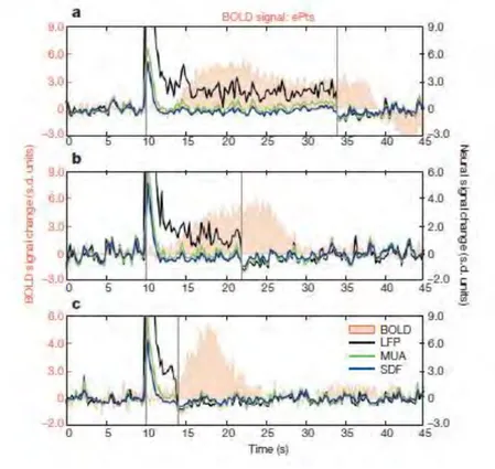
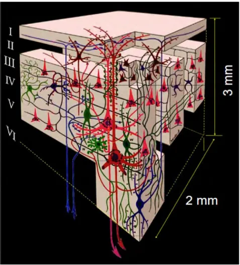
Après une introduction générale sur le système visuel et après avoir passé en revue les principales connaissances accumulées jusqu’à présent sur l’intégration des disparités binoculaire par le système visuel du primate et présenté les objectifs généraux de la thèse, j’introduis l’approche expérimentale principalement utilisée dans le cadre de mes travaux de recherche dans un troisième chapitre. Nous proposons en effet d’utiliser la neuroimagerie fonctionnelle (IRMf) chez le primate non humain afin de pouvoir faire le lien entre les études unitaires pratiquées chez le macaque et les études de neuroimagerie effectuées chez l’humain. Cette approche représente un challenge en soi de par la nécessité de devoir conditionner les animaux à rester immobiles dans le scanner et à effectuer une tâche comportementale, mais aussi de par le besoin de développer des analyses et outils spécifiques pour l‘espèce étudiée afin d’avoir une bonne mesure du signal. Dans ce chapitre méthodologique, je mentionne les principes physiques fondamentaux de l’imagerie par résonnance magnétique (IRM) et les différents types de séquences qui peuvent être utilisées pour générer des contrastes, qui reflètent différents niveaux d’intensité du signal de résonnance magnétique dans les tissus étudiés et parmi eux le contraste BOLD utilisé dans le cas de l’IRMf. Je détaille ensuite la nature du signal mesuré dans nos études en neuroimagerie, le signal BOLD, qui repose sur une comparaison des niveaux d’hémoglobine oxygénée et désoxygénée présentes dans le sang. J’évoque les différences entre le signal BOLD et les autres signaux d’activités cérébrales qui sont traditionnellement mesurés chez le macaque : les potentiels de champs locaux et les potentiels d’action émis par une ou plusieurs cellules nerveuses. Cela me permet ensuite d’enchaîner sur le développement de l’IRMf chez le macaque, des différentes stratégies adoptées par les groupes de recherche pratiquant cette technique chez le singe et de
xii sa pertinence pour faire le lien entre les études d’électrophysiologie réalisées chez le macaque, et qui enregistrent un signal plus précis mais très local (potentiels de champs locaux et potentiels d’actions neuronaux) et les études de neuroimagerie réalisées chez l’humain, qui donnent un aperçu plus global de l’activité cérébrale.
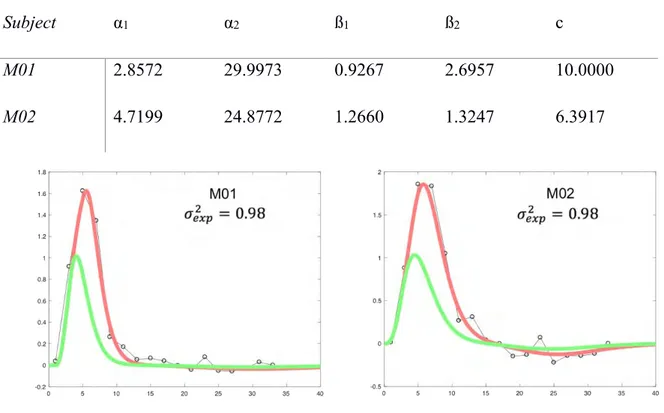
Je souligne le fait que des traitements spécifiques à la fois du signal et statistiques ont dû et sont continuellement en train d’être développés pour rendre possible la neuroimagerie fonctionnelle chez le macaque. Par ailleurs, l’idée de l’IRMf est de considérer le niveau d’oxygénation des aires cérébrales comme marqueur de leur activité, il s’agit donc d’une mesure indirecte et qui présente un décours temporel spécifique, représentée par une fonction de réponse hémodynamique (HRF). Afin de mieux estimer l’activité cérébrale en réponse à des stimuli, il est nécessaire de déterminer la dynamique de la réponse BOLD et donc la HRF. Je présente la façon dont nous avons procédé pour estimer la HRF dans chacun de nos sujets macaques et comment nous l’implémentons dans nos modèles statistiques. Comme preuve de concept, je développe les résultats de deux études qui ont été réalisées dans l’équipe et auxquelles j’ai en partie participé. La première étude est un travail d’équipe réalisé sur plusieurs années et qui a permis le développement de l’IRM singe au CerCo. Il s’agit d’un travail de recherche portant sur les aires cérébrales impliquées dans le traitement du flux optique. Ce travail, qui a fait l’objet d’une publication en 2017 (Cerebral Cortex) et a pu montrer qu’il existe une différence de traitement du flux optique selon que celui-ci est compatible ou non avec la locomotion. À la suite de ces débuts fructueux et dans le cadre de la thèse d’un précédant doctorant, la seconde étude, en cours de révision, a donné de nouveaux outils d’analyse à l’équipe en s’intéressant aux propriétés rétinotopiques des aires visuelles et notamment au sein du cortex pariétal postérieur. J’ai ainsi pu réutiliser les délimitations rétinotopiques des aires visuelles pour réaliser certaines analyses de mes données fonctionnelles.
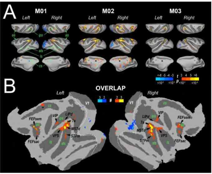
xiii Le chapitre suivant (chapitre 4) est le premier chapitre expérimental. Il porte sur une forme d’intégration temporelle des disparités binoculaires. Il s’agit d’une étude en neuroimagerie fonctionnelle, présentée à plusieurs conférences internationales et qui a été acceptée pour publication dans le journal Cerebral Cortex. Nous avons adapté deux études réalisées chez l’humain afin de caractériser chez le macaque le réseau cortical impliqué dans le traitement du mouvement tridimensionnel, mouvement défini ici par un changement des valeurs de disparités binoculaires à travers le temps. Nous avons contrasté les réponses BOLD à deux conditions expérimentales pour lesquelles l’information tridimensionnelle n’était disponible que lorsque vue par les deux yeux simultanément. La première condition représentait un mouvement 3D tel qu’émis par un objet se rapprochant ou s’éloignant de l’observateur tandis pour que la deuxième, la condition contrôle, nous avions mélangé les images vidéo de la première condition avec pour résultat une alternation saccadée de plans dans l’espace. Nos analyses ont permis de montrer qu’au sein de chaque hémisphère pour les deux sujets macaques ayant fait l’expérience trois aires ont été sélectivement plus activées par le mouvement 3D (appelé Cyclopean StereoMotion ou CSM dans notre étude) que par son contrôle. Ces aires étaient localisées sur la berge inférieure du sillon temporal supérieur (CSMSTS), sur le gyrus inféro- temporal (CSMITG), et dans la partie caudale du sillon
intra-pariétal postérieur (CSMPPC). À l’aide d’analyses rétinotopiques, nous avons pu montrer que
l’aire CSMSTS ne se trouvait pas dans le cluster MT, un groupe de 4 aires cérébrales associées
au traitement du mouvement, mais qu’elle se trouvait à une position plus antérieure. Nous avons également démontré que certaines des aires de ce cluster MT avaient des réponses significativement plus élevées pour le mouvement 3D que pour le stimulus contrôle, et notamment les aires MSTv et FST. Nous n’avons pas trouvé de préférence marquée pour le mouvement 3D dans l’aire MT allant dans le sens des résultats obtenus lors d’enregistrements électrophysiologiques chez le macaque et qui suggèrent une sélectivité au mouvement 3D
xiv principalement basée sur un autre indice : les différences de vélocité interoculaires. En utilisant des stimuli révélant la sélectivité au mouvement planaire (ou mouvement bidimensionnel, 2D), nous avons pu révéler qu’à la fois CSMSTS et CSMITG répondaient au
mouvement 2D, mais que CSMPPC semblait montrer une sélectivité unique pour le
mouvement 3D.
De façon intéressante, notre aire CSMITG se trouve à la jonction ou à l’intérieur, selon les
hémisphères testés, de l’aire V4 et potentiellement de l’aire V4A, aire documentée comme répondant à la disparité et au mouvement et appartenant à un autre cluster, que nous n’avons malheureusement pas pu définir à partir de nos données. On peut néanmoins souligner un résultat similaire dans une étude en IRMf réalisée chez des sujets humains qui a trouvé que les aires LO-1 et 2, considérées comme potentielles aires homologues de V4A, répondaient aussi au mouvement 3D, appuyant davantage une possible homologie.
Enfin, la troisième aire, CSMPPC, du fait de sa localisation en amont d’aires impliquées dans
le traitement des structures 3D et sensibles à la profondeur kinétique, pourrait être une aire complémentaire à l’aire caudale intra-pariétale (CIP) située sur la berge opposée du sillon intra-pariétal postérieur. En effet, l’aire CIP n’a pas montré de sensibilité à la profondeur kinétique, que l’on peut rapprocher du mouvement 3D, mais est connue pour répondre aux orientations spatiales et arrangements d’éléments dans l’espace. L’aire CSMPPC pourrait ainsi être son pendant temporel du traitement des disparités binoculaires.
Plus globalement et considérés dans leur ensemble, nos résultats suggèrent que les aires corticales impliquées dans le traitement du mouvement 3D sont partiellement communes au macaque et à l’humain.
xv Dans le second chapitre expérimental (chapitre 5), deux études sont présentées, une étude en neuroimagerie chez le macaque et une étude de psychophysique à la fois chez le macaque et chez l’humain. Toutes deux ont vocation à déterminer si le traitement spatial des disparités, déjà assez bien documenté, ne pourrait pas être influencé par les régularités spatiales présentes dans les scènes visuelles. Afin de tester cette hypothèse, nous avons, dans une première expérience, enregistré le signal BOLD en réponse à différentes surfaces orientées dans la profondeur. Ces surfaces étaient inclinées soit autour de l’axe horizontal (‘slants’) vers l’avant ou vers l’arrière, soit autour de l’axe vertical (‘tilts’) vers la gauche ou vers la droite. Nous avons contrasté les réponses à ces orientations avec celles à une condition contrôle pour laquelle il n’y avait pas de percept 3D (condition décorrélée) mais qui était identique aux autres conditions lorsqu’elles étaient vues de façon monoculaire, prenant alors la forme de simples nuages de points. Nous avons dans un premier temps cartographié l’étendue du réseau répondant aux disparités corrélées en opposant nos orientations 3D, que celles-ci soient autour de l’axe horizontal ou de l’axe vertical, à la condition décorrélée. Afin de préciser l’importante étendue des aires significativement activées pour les disparités corrélées, nous avons réalisé une analyse rétinotopique dans les aires visuelles précoces (V1, V2, V3, V4), au sein du cluster MT (MT, MSTv, V4t, FST), au sein du cluster PIP récemment redéfini par un ancien doctorant de l’équipe (PIP1, PIP2, CIP1, CIP2), et au niveau de trois aires plus dorsales (V3A, V6, V6A). De façon inattendue, nous avons trouvé de légères différences selon le type d’orientation avec des activations plus fortes pour les disparités corrélées lorsqu’on considérait les orientations autour de l’axe horizontal (‘slant’) que lorsqu’on considérait les orientations autour de l’axe vertical (‘tilt’). En considérant uniquement les aires répondant de façon systématique aux disparités corrélées pour les deux types d’orientation, nous avons pu trouver un réseau similaire à celui décrit dans la littérature avec notamment les aires MT, MSTv, CIP1, CIP2, PIP2, V3A et V6A qui répondaient plus
xvi fortement aux disparités corrélées qu’aux disparités non corrélées. De façon intéressante, l’aire PIP1 ne ressortait jamais dans plus de 2 hémisphères sur 4 comme répondant plus fortement aux disparités corrélées quel que soit le type d’orientation considérée, contrastant ainsi avec les trois autres aires du cluster PIP qui elles répondaient de façon systématique aux disparités corrélées en considérant les deux types d’orientations 3D.
Dans un deuxième temps, nous nous sommes intéressés à l’influence des statistiques naturelles sur les activations cérébrales en réponses aux orientations 3D. Afin de déterminer si les réponses étaient plus fortes pour l’orientation la plus fréquemment rencontrée dans l’environnement, nous avons uniquement considéré les aires précédemment décrites comme répondant de façon systématique aux disparités corrélées sans influence de l’orientation 3D considérée. Afin de mettre en évidence une éventuelle préférence pour ce type d’inclinaison, nous avons comparé deux à deux nos deux types d’orientation (‘slants’ et ‘tilts’) : surfaces inclinées vers l’avant versus surfaces inclinées vers l’arrière, et surfaces orientées vers la droite versus surfaces orientées vers la gauche. Nous nous attendions à trouver un biais pour les surfaces inclinées vers l’arrière (‘slant’) avec des activations plus fortes pour l’inclinaison arrière que pour l’inclinaison avant, cette configuration arrière étant alignée avec l’orientation du sol dans les scènes naturelles et donc plus fréquente dans l’environnement visuel. En revanche, nous n’attendions aucune différence entre les surfaces orientées vers la gauche et vers la droite, ces orientations ne présentant pas de différence dans leurs fréquences d’apparition au sein des scènes visuelles. Étonnamment, lorsque nous avons considéré les cartes d’activations des contrastes BOLD effectués (avant versus arrière et droite versus gauche), nous avons trouvé des activations plus fortes pour l’inclinaison arrière chez un seul de nos sujets macaques, et une absence de différence chez le second sujet. Nous n’avons par contre pas trouvé de différence entre les orientations droite et gauche, et ce pour nos deux sujets, ce qui était attendu. Des analyses rétinotopiques chez le sujet présentant un biais pour
xvii les inclinaisons arrière ont révélé que c’était principalement au niveau du cluster PIP que les activations étaient les plus biaisées, c’est-à-dire que c’était au niveau des aires de ce cluster que les activations étaient plus fortes pour les surfaces inclinées vers l’arrière. Ces analyses n’ont pas permis de trouver de résultats similaires pour le deuxième sujet. Nous avons ensuite essayé de considérer l’élévation, en divisant nos stimuli d’inclinaisons 3D (‘slants’) en trois parties : une partie supérieure, correspondant au champ visuel supérieur (>2°), une partie médiane, correspondant à la zone centrale du champ visuel (±2°), et une zone inférieure, correspondant au champ visuel supérieur (< -2°). L’idée était d’adresser l’hypothèse que considérer les activations au niveau du stimulus dans sa globalité ne permettait peut-être pas de révéler des biais pour certaines orientations. Nous avons donc essayé de voir si les scores de t obtenus pour chaque inclinaison (arrière et avant) étaient plus élevés pour les disparités dites croisées (donnant un niveau de profondeur en avant du point de fixation) dans le champ visuel inférieur, et plus élevés pour les disparités décroisées (niveau de profondeur en arrière du point de fixation) dans le champ visuel supérieur, ce qui correspond à une configuration de plan incliné vers l’arrière. Si nous avons à nouveau pu confirmer que notre premier sujet macaque montrait un biais pour les surfaces inclinées vers l’arrière, et non un biais général pour les disparités croisées, cette méthode n’a pas non plus permis de montrer que c’était aussi potentiellement le cas chez notre deuxième sujet. Nous ne sommes pas surs de l’origine d’une telle différence entre nos sujets. Des analyses supplémentaires seront donc nécessaires, telle que l’utilisation d’une approche multivariée par comparaison de motifs d’activation pour passer outre les limitations des analyses univariées que nous avons effectuées jusqu’à présent. À défaut de pouvoir conclure sur une influence des statistiques naturelles sur l’activité cérébrale, nous avons néanmoins pu décrire de façon robuste le réseau cortical impliqué dans le traitement spatial des disparités binoculaires chez nos deux sujets. Nous avons ainsi trouvé sept aires rétinotopiques qui répondaient plus fortement à nos conditions corrélées
xviii (orientations autour de l’axe horizontal et autour de l’axe vertical) qu’à la condition contrôle décorrélée, en accord avec la littérature.
La deuxième étude présentée dans ce chapitre expérimental est une étude de psychophysique réalisée à la fois chez l’humain et chez le macaque. L’objectif était de mesurer la composante verticale de l’horoptère de nos sujets, c’est-à-dire la région de l’espace dans laquelle la stéréoacuité est la plus fine. Concrètement, il s’agit de déterminer la localisation des points rétiniens correspondants qui sont les points dans l’espace perçus comme superposés au niveau de leur projections rétiniennes et qui permettent de faire correspondre entre elles ces deux projections rétiniennes, donnant naissance au percept 3D. Plusieurs études chez l’humain ont suggéré que la position de ces points correspondants sur l’axe vertical, inclinés vers l’arrière par rapport au plan de fixation, pourrait refléter les statistiques naturelles. Bien que le macaque soit un modèle du système visuel humain, nous ne savons pas si cette inclinaison de l’horoptère vertical est aussi présente chez cette espèce. Nous avons donc adapté un protocole auparavant réalisé chez l’humain et mesuré expérimentalement la localisation des points correspondants chez un sujet macaque et chez huit sujets humains. La tâche expérimentale consistait à fixer un point central pendant qu’apparaissaient successivement et de façon brève deux barres présentées chacune dans un œil. À la suite de cette présentation de barre, les sujets devaient indiquer la direction du mouvement apparent perçu, mouvement résultant de l‘apparition successive des deux barres. La distance entre les barres variait au cours du temps, soit de façon constante pour le sujet macaque, soit de façon adaptée via une procédure en staircase (variation de la distance des barres en fonction de la réponse donnée par les sujets) chez les sujets humains. Par ailleurs, les barres étaient présentées à différentes excentricités sur l’axe vertical du champ visuel. L’expérience se terminait lorsque les réponses des sujets pour une distance de barre donnée et pour chaque excentricité testée stagnaient autour du niveau de la chance, reflétant alors des réponses au
xix hasard et donc une absence de perception du mouvement. Ce sont ces distances de barres pour lesquelles un mouvement apparent n’est plus perçu qui nous intéressent. Cela signifie en effet que les barres sont perçues comme superposées par nos sujets et les localisations rétiniennes stimulées par ces barres sont alors dites correspondantes.
La mesure de ces points correspondants à différentes excentricités a permis de confirmer une inclinaison de la composante verticale de l’horoptère chez nos sujets humains, avec des variabilités inter-individuelles significatives. Surtout, et malgré le fait que toutes les mesures n’aient pas fini d’être collectées cette mesure expérimentale réalisée pour la première fois chez un sujet macaque a révélé qu’une telle inclinaison de l’horoptère était potentiellement aussi présente chez cette espèce. Cette inclinaison est également comparable à celle décrite chez l’humain et retrouvée chez nos huit participants humains. Cette absence de différence entre les deux espèces, attendues si l’on considère les différences de statistiques naturelles auxquelles elles sont exposées, semble favoriser l’idée que la relation entre la distance interoculaire et la hauteur des yeux serait un meilleur facteur explicatif de la forme de l’horoptère vertical. Cette hypothèse permettrait notamment de considérer les mesures indirectes (enregistrements électrophysiologiques des champs récepteurs) de l’horoptère vertical qui avaient été réalisées dans les années 1970 chez le chat et la chouette et qui suggèrent que ces deux espèces ont des inclinaisons similaires mais très différentes de celles trouvées chez l’humain et maintenant chez le macaque.
Ces résultats devront évidemment être répliqués chez un autre macaque pour pouvoir réellement conclure sur le rôle de l’expérience visuelle sur la forme empirique de l’horoptère. Néanmoins, ils ouvrent déjà la voie à de nouvelles hypothèses et prédictions.
xx Pour conclure sur ces différents travaux effectués dans le cadre de ma thèse, le dernier chapitre de ce manuscrit (chapitre 6) comprend la discussion générale dans laquelle les résultats sont remis dans le contexte plus général de l’intégration par le système visuel et au niveau cortical principalement de la disparité binoculaire. La possibilité d’un recouvrement au moins partiel des réseaux corticaux impliqués dans les dimensions spatiale et temporelle de l’intégration binoculaire est discutée, de même que leurs implications au niveau des différentes voies visuelles connues. Finalement, des pistes de réflexions pour de futures études relevant de la psychophysique ou de la neuroimagerie et visant à surmonter les limitations des études menées lors de cette thèse sont proposées. Également, certaines limitations au niveau des connaissances actuelles sont évoquées.
xxii
Table of Contents
Acknowledgements ... i Abstract ... v Résumé ... vi Résumé substantiel en langue française ... vii Chapter I – General introduction to the visual perception in the primate brain ... 1 The visual system: from the retina to early visual areas ... 2 From early visual areas to higher visual areas: two pathways ... 14 Three-dimensional vision and binocular disparity ... 16 Chapter II – Context of the thesis: Integration of binocular disparities in the primate brain . 21 Disparity processing and binocular integration ... 22 Absolute versus relative disparity ... 27 Disparity configuration and natural statistics ... 31 Temporal integration of binocular disparities ... 35 Methodological approach... 36 Chapter III – Monkey fMRI - Methodology ... 38 The BOLD signal ... 39 Physics of (functional) magnetic resonance imaging ... 39 Nature of the BOLD signal and how it relates to the underlying neural activity ... 42 BOLD signal vs. MION-enhanced signal ... 49 Pre-processing steps and general linear model (GLM) ... 50 Optimising the HRF estimation and data pre-processing to improve the SNR ... 52 Estimating the individual haemodynamic response function (HRF) ... 52 Constant improvement of our methods: Complexity and success ... 54 Chapter IV – Temporal integration of binocular disparity: The case of motion-in-depth ... 61 General introduction ... 62 First study: Steremotion processing in the non-human primate (accepted article) ... 66
xxiii Introduction ... 66 Materials and Methods ... 69 MRI recordings ... 72 Data analysis ... 74 Results ... 81 Discussion ... 94 Conclusion ... 103 Chapter IV – Spatial integration of binocular disparity: Influence of natural statistics ... 105 Content of this chapter ... 106 Second study: Spatial disparity gradients ... 107 Introduction ... 107 Material and methods ... 109 MRI recordings ... 112 Data analysis ... 113 Statistical analyses ... 116 Orientation biases... 125 Differential activations with elevation? ... 130 Discussion ... 134 Conclusion ... 136 Third study: Measure of the horopter in human and in macaque ... 137 Introduction ... 137 Experimental setups ... 142 Results ... 147 Discussion ... 155 Chapter V – General discussion: What did we learn about the integration of binocular disparities? ... 158
xxiv Overlapping cortical networks between temporal and spatial integration of binocular disparities: the case of the PIP cluster ... 161 Dorsal versus ventral visual pathways ... 163 Limitations and future directions ... 166 Linking cortical activation to behavioural responses ... 166 Functional connectivity within the revealed network ... 167 Modularity of the primate brain ... 168 Summing it all up with a nice quotation ... 171 References ... 173 Appendix I – Consent form for the horopter experiment conducted in humans ... ii Appendix II – Cottereau, B. R., Smith, A. T., Rima, S., Fize, D., Héjja-Brichard, Y., Renaud, L., Lejards, C., Vayssière, N., Trotter, Y., & Durand, J.-B. (2017). Processing of Egomotion-Consistent Optic Flow in the Rhesus Macaque Cortex. Cerebral Cortex, 1–14. ... vii
xxv
List of figures
Figure 1: Anatomy of the eye. ... 3 Figure 2: Retina cell layers. ... 5 Figure 3: Phototransduction. ... 6 Figure 4. Projections of ganglion cells to the lateral geniculate nucleus (LGN). ... 11 Figure 5: Visual pathway, from the retina to the primary visual cortex. ... 12 Figure 6: Hierarchical organisation of the visual system ... 17 Figure 7: Stereopsis is present in many different species. ... 18 Figure 8. A classic random-dot stereogram as described by Julesz (1971). ... 24 Figure 9. Schematised disparity tuning curves of two neurons in the primary visual cortex. . 25 Figure 10. The disparity energy model. ... 27 Figure 11. Absolute and relative disparities. ... 28 Figure 12. Centre-surround stimuli to assess responses to absolute vs. relative disparities. ... 29 Figure 13. Responses of three neurons recorded at two different surround disparities. ... 30 Figure 14. Depth orders. Three orders of depth can be defined and result in different types of disparity-defined stimuli as illustrated here.. ... 32 Figure 15: The BOLD signal reflects variations in oxygen consumption and modification of blood flow. ... 44 Figure 16: Simultaneous neural and haemodynamic recordings from a cortical site (in the striate cortex) showing transient neural response. ... 45 Figure 17: Illustration of the different types of cells and synapses that are comprised in a cube that has the equivalent size of one voxel. ... 46 Figure 18: MRI-compatible chair for macaque. ... 49 Figure 19. Characterisation of the haemodynamic response function (HRF). ... 54
xxvi Figure 20: A) Statistical parametric maps for the EC versus EI contrast in monkeys M01, M02, and M03. B) Map of overlap between significant activations in the EC versus EI contrast across the 3 monkeys... 56 Figure 21: A) Average sensitivity ratio (%) between the responses to the EC and EI conditions. B) Schematic localization of the 8 areas on the F99 template. ... 57 Figure 22: Mean PRF results (4 hemispheres) projected on the right inflated cortical surface of the F99 monkey template. ... 58 Figure 23: Assessing the contribution of the two binocular cues to motion-in-depth ... 63 Figure 24. Stimulus design and experimental protocol. ... 71 Figure 25. Activations for the contrast between Cyclopean Stereomotion (CSM) and its temporally scrambled version (TS) for M01.. ... 82 Figure 26. Activations for the contrast between Cyclopean Stereomotion (CSM) and its temporally scrambled version (TS) for M02. ... 83 Figure 27. Activations for the contrast between Cyclopean Stereomotion (CSM) and its temporally scrambled version (TS) projected onto individual cortical surfaces and on the F99 template. ... 85 Figure 28. A) Retinotopic mapping of the Superior Temporal Sulcus (STS) for M01 and delimitation of the MT cluster areas. B) Activations for the contrast between Cyclopean Stereomotion (CSM) and its temporally scrambled version (TS) projected on the individual surfaces of M01, for both left and right hemispheres. C) Difference in percent signal change (∆PSC) between the CSM and TS conditions in retinotopic areas ... 88 Figure 29. A) Retinotopic mapping of the Superior Temporal Sulcus (STS) for M02 and delimitation of the MT cluster areas. B) Activations for the contrast between Cyclopean Stereomotion (CSM) and its temporally scrambled version (TS) projected on the individual
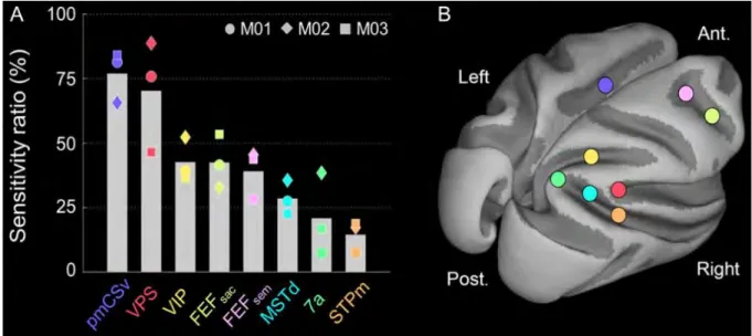
xxvii surfaces of M02, for both left and right hemispheres. C) Difference in signal change (∆PSC) between the CSM and TS conditions in retinotopic areas ... 89 Figure 30. Sensitivity to 2D motion in CSMSTS, CSMITG, and CSMPPC.. ... 91 Figure 31. Selectivity to 3D and 2D motion within the STS.. ... 93 Figure 32. Activations for the contrast between Cyclopean Stereomotion (CSM) and its temporally scrambled version (TS) for M01 and M02. ... 100 Figure 33. A) Retinotopic mapping of the Superior Temporal Sulcus (STS) for M01 and delimitation of the MT cluster areas. B) Average eccentricities for the four areas of the MT cluster and for CSMSTS for both subjects. C) Retinotopic mapping of the Superior Temporal Sulcus (STS) for M01 and delimitation of the MT cluster areas. D) Average pRF sizes for the four areas of the MT cluster and for CSMSTS for both subjects ... 101 Figure 34. Ocular behaviour.. ... 103 Figure 35. Experimental protocol. ... 111 Figure 36. Activations for the contrast Correlated (GS+nGS) vs. Uncorrelated for M01. .... 117 Figure 37. Activations for the contrast Correlated (GS+nGS) vs. Uncorrelated for M02. See Figure 36 for the details of the legend. ... 118 Figure 38. Activations for the contrast Correlated (RT+LT) vs. Uncorrelated for M01 ... 119 Figure 39. Activations for the contrast Correlated (RT+LT) vs. Uncorrelated for M02 ... 120 Figure 40. Difference in signal change (∆PSC) between correlated (GS+nGS) and uncorrelated conditions in early visual areas and in the MT cluster ... 122 Figure 41. Difference in signal change (∆PSC) between correlated (GS+nGS) and uncorrelated conditions in the PIP cluster and in V3A, V6, and V6A areas. ... 123 Figure 42. Activations for the contrast GS > nGS for M01. ... 126 Figure 43. Activations for the contrast GS>nGS on the left and for the contrast nGS>GS on the right for M02.. ... 127
xxviii Figure 44. Difference in signal change (∆PSC) between the ground-aligned slant (GS) and the non-ground aligned slant conditions in the PIP cluster.. ... 128 Figure 45. Activations for the contrasts RT > LT on the left and LT>RT on the right for M01. ... 129 Figure 46. Activations for the contrasts RT > LT on the left and LT>RT on the right for M02. See Figure 45 for details of the legend. ... 129 Figure 47. Predictions of t-score patterns as a function of elevation for different disparity preferences. ... 132 Figure 48. Difference in t-score values between GS and nGS conditions as a function of the elevation for M01.. ... 133 Figure 49. Difference in t-score values between GS and nGS conditions as a function of the elevation for M02.. ... 134 Figure 50. Geometric and empirical horopters. ... 138 Figure 51. A) Eye-and-scene tracking device and weighted combinations of the four different activities (median horizontal disparities). B) Distributions of preferred horizontal disparity grouped by upper and lower visual field. ... 140 Figure 52. Apparent motion paradigm for the measurement of corresponding points. ... 144 Figure 53. Predicted psychometric curves. ... 147 Figure 54. Data from Observer 1. ... 148 Figure 55. Location of corresponding points for subjects 2 to 4.. ... 150 Figure 56. Fitted curves for the different eccentricities at which corresponding points were measured. ... 151 Figure 57. Non-corrected locations of corresponding points for the macaque subject ... 152 Figure 58. Non-corrected locations of corresponding points for the macaque subject for even (left panel) and odd (right panel) trials. ... 152
xxix Figure 59. Fitted curves for the different eccentricities at which corresponding points were measured for the even trials.. ... 153 Figure 60. Fitted curves for the different eccentricities at which corresponding points were measured for the odd trials. ... 153 Figure 61. PIP cluster as defined in the wide-field retinotopic study mentioned in Chapter III. (Rima et al., under review). ... 162 Figure 62. Regions sensitive to structural and positional stereoscopic information are projected onto the flattened representations of left and right IPS... ... 163 Figure 63. Schematic representation of known functional interactions between different areas from the dorsal and ventral pathways.. ... 168 Figure 64. Different visual and oculomotor cues can be used by the primate visual system to compute a 3D percept.. ... 170
xxx
List of tables
Table 1: Parameter values of the HRF for each individual ... 54 Table 2. MNI coordinates (in mm) of the local maxima for the 3 regions that were significantly more responsive for the CSM condition than for the TS control in the two hemispheres of the two animals. ... 84 Table 3. Number of hemispheres that pass the significance threshold for each retinotopic areas and for each contrast.. ... 124 Table 4: Participants characteristics for the measurement of corresponding points. ... 145 Table 5. Interspecies comparisons of the optimal shear angles. ... 155
1
Chapter I –
General introduction to the visual perception
in the primate brain
2
From the photon that hits the retina to the visual interpretation of our
environment
The visual system: from the retina to early visual areas
Whilst we heavily rely on our vision to interact with our environment and perform everyday life actions, most of the time we do not realise how complex the visual machinery might be. What underlies this ability that most species have to visually perceive the world? How does a nervous system, the brain in our case, manage to make sense of the light information that comes and hits the retina?
These questions are far from being new as already Plato and Galen had their own views on the matter. From the extramission theory, once claiming that the eye emits light to encompass objects, to the intromission theory introduced during the Islamic Golden Age by Ibn al-Haytham (Alhazen) and Ibn Sina (Avicenna) that was finally stating that the eye is using the light to provide visual perception, it was only during the early 17th century with Kepler’s work that we approached the idea of a camera obscura, with an image being projected on the retina.
The metaphor of the camera works well to grasp the anatomy of the mammal eye and explain the role of the different elements that compose it.
As illustrated on Figure 1, the light –in the form of an electromagnetic wave – first goes through the cornea, a fixed transparent membrane in charge of about 70% of the light refraction and that covers the iris and the pupil. The muscular action of the iris will allow more or less light to enter the eye by constricting (miosis) or dilating the pupil (mydriasis), a phenomenon also known as the pupillary light reflex. The second step is the aqueous humour, a watery fluid that provides nutrients to the cornea.
3 Figure 1: Anatomy of the eye.
The mammal eye is made of different elements that help refract the light to be focused on the retina. The light, in the form of an electromagnetic wave, first goes through the cornea, in charge of about 70% of refraction, crosses the aqueous humour, a watery liquid that provides nutrients to the cornea, then goes through the lens, a biconvex structure that further refracts the light by accommodating, and finally crosses the vitreous humour, a sort of jelly matter that gives its round shape to the eye, before hitting the retina and the different cells that compose it. The most detailed information is projected onto one specific part of the retina: the fovea, where signal processing is finer, due to the asymmetrical retina cell distribution (detailed further in the text). Image retrieved from https://www.umkelloggeye.org/conditions-treatments/anatomy-eye
The light will then go through the lens, a biconvex structure composed of different layers and that further helps to refract the light by accommodating under the action of ciliary muscles,
4 doing the same work as the focus of a camera. Ciliary muscles will contract for a short distance, thus bending and thickening the lens, giving it a strong refraction power, and they will relax for a far distance, then stretching the lens. Finally, the luminous information will cross the vitreous humour, a sort of jelly that gives the eye its round shape before reaching the retina and the cells that it is made of (see e.g. Masland, 2001).
Located in the back of the eye, the retina is in charge of transforming the light information into a signal that will be interpreted by the brain, that is an electric signal. Among the different cell layers retina is made of (see Figure 2), the photoreceptor layer represents the initial step of signal conversion. Photoreceptors are divided into two categories: rods and cones. Rods are mostly responsible for dim light vision and represent the majority of photoreceptors (95% of them, that is about 120 million), whilst cones are more sensitive to bright and coloured light, being themselves divided into three different types: short wave-length (blue colour), medium wave-wave-length (green colour), and long wave-wave-length (red colour) sensitive cones. The distribution of rods and cones varies across the retina, with most cones being in the centre of the retina, at the fovea level, and rods being more highly dense in the periphery surrounding the fovea. A chemical cascade reaction, known as photo transduction (see Figure 3 for more details), is the result of photon detection within the outer part of the photoreceptor cells that contain photoreceptor pigments (rhodopsin in rods and photopsin in cones), leading to an hyperpolarisation of photoreceptor cells that further conveys the now-electric message, in the form of a membrane potential, to the next layer made of bipolar and horizontal cells.
From photoreceptors to bipolar cells, the information is compressed due to a lesser number of bipolar cells than of photoreceptor cells and the resolution varies depending on the type of photoreceptors. High numbers of rods in the periphery of the retina converge onto single bipolar cells, whereas cone information from the retina is less compressed, thus giving rise to
5 a high-resolution vision at the fovea level. This difference will be preserved at the brain level, since proportionally more optic nerve fibres, made of the axons of ganglion cells, will conduct information from the cones, giving a primary importance to the information projected on the fovea.
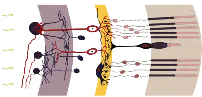
Figure 2: Retina cell layers.
Light (yellow arrows on the left) goes through the different layers in the retina before reaching the photoreceptor layer (beige layer, on the very right). The information encoded by photoreceptors (cones in the fovea and rods in the periphery) is then back propagated to the bipolar and horizontal cells (the outer plexiform layer, in yellow) and further sent to the ganglion cells (the inner plexiform layer, in purple) before leaving the retina through optic nerve fibres made of the axons of ganglion cells. Image retrieved from Wikipedia Commons:
https://commons.wikimedia.org/wiki/File:Retina-diagram.svg (vectorisation of picture from Ramon y Cajal by Chris).
Each retina cell encodes a spatial localisation of the visual space, that is one cell’s baseline state will be modified in response to the presence of light in one part of the visual field only, leading to a modification of the cell’s membrane potential or a generation of action
6 potentials. This cell sensitivity area is its receptive field. The size of those receptive fields varies accordingly to the visual cell hierarchy, becoming bigger and bigger as one goes up the layers of the visual system. Photoreceptors are their own receptive field, as they will be triggered by luminous information received in their outer segments localised in one physical point of the retina on which visual space is projected. Photoreceptors are connected to bipolar cells and they will then represent the receptive fields of those bipolar cells. Several bipolar cells are also connected to a ganglion cells and they will again compose the receptive field of this ganglion cell. The receptive field of the ganglion cell is thus a collection of the sensory inputs that are received by all the photoreceptors that are synapsing with the bipolar cells that are connected to the ganglion cell. This convergence process will continue up to brain neuron cells, leading to bigger and bigger receptive fields (see e.g. Briggs, 2017).
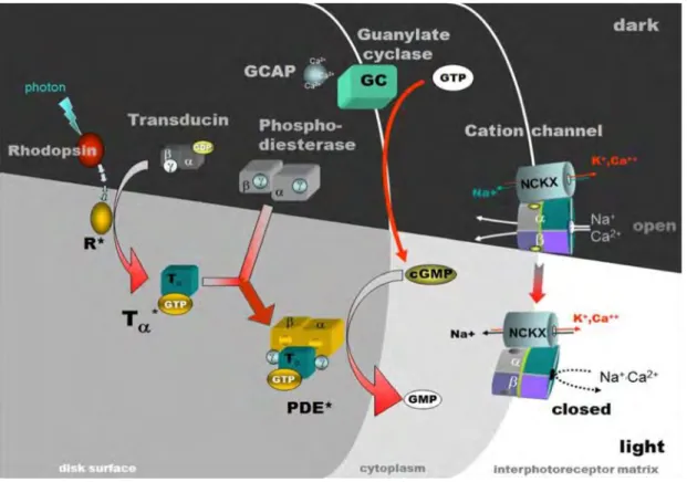
Figure 3: Phototransduction.
Photoreceptors baseline state is within dark conditions, photoreceptors are then depolarised due to high level of cGMP keeping sodium gates open. This allows potassium ions to get out
7 of the cell and sodium to get in, creating what is called a dark current. A neurotransmitter, glutamate, is then released by the photoreceptor. The action of glutamate is to hyperpolarise ON-centre bipolar cells and to depolarise OFF-centre bipolar cells (for sake of simplicity, we will not mention the horizontal cell pathway). Once a photon is detected by a photopigment present in the disks of the outer segment of a photoreceptor (here, the rhodopsin), it triggers a whole chemical cascade as illustrated on the figure. Briefly, the retinal component (a vitamin A derivative) of the rhodopsin molecule becomes activated (R*), changing configuration from 11-cis to all-trans. To balance this change, opsin, the other component of rhodopsin, also undergoes a configuration change becoming metarhodopsin II. Metarhodopsin II then activates the transducing protein, causing its dissociation from GDP and its binding to GTP. The alpha subunit of transducing Tα* dissociates from the other subunits but remains attached to the binding GTP. This complex will then activate the cGMP-hydrolysing phosophodiesterase (PDE*) responsible for the degradation of cGMP in GMP. As a consequence, cGMP concentration within the cell decreases, leading to the closing of cGMP-dependent sodium gates, thus stopping the dark current and causing the hyperpolarisation of the photoreceptor cell. Glutamate is no longer released in big quantities and ON-centre bipolar cells depolarise whilst OFF-centre bipolar cells hyperpolarise. Image copyright: Wolfgang Baehr (https://pubmed.ncbi.nlm.nih.gov/18193635/).
Receptive fields are not simply defined as a region getting excited by light. From bipolar cells onwards they also have an ON-OFF organisation, having one or several excitatory parts and one or several inhibitory parts. Their shape varies from being circular at the retina level to being more elongated once at the cortex level, becoming more sensitive to the light orientation.
Bipolar cells for instance have an antagonist centre-surround organisation, with two possible configurations: an ON-centre associated with an OFF-surround or an OFF-centre coupled with an ON-surround (see e.g. Dacey, Crook and Packer, 2017). Located between photoreceptors and bipolar cells, horizontal cells will selectively inhibit the information of some photoreceptors, only allowing strongly emitting photoreceptive cells (i.e.
8 photoreceptors receiving the highest amount of light) to transmit their signal to the bipolar cell they are connected to, thus increasing the signal-to-noise ratio. They are directly involved in the centre-surround organisation of the bipolar cells as they mediate the surround activity of the bipolar cells. The ON-OFF configuration of bipolar cells and the lateral inhibition property of horizontal cells represent the first step in the detection of edges and contrasts in the visual information received at the level of the retina.
Ganglion and amacrine cells compose the last step before the information leaves the retina through the optic nerve fibres made of the axons of ganglion cells.
Part of the inner plexiform layer like ganglion cells, amacrine cells are interneurons that are involved in integrating and modulating temporal information to transmit it to the ganglion cells. They might also play a similar role as of the horizontal cells in varying the signal from adjacent ganglion cells to enhance signal-to-noise ratio.
Ganglion cells are subdivided into three main categories: magnocellular (M-type), parvocellular (P-type), and koniocellular (K-type) ganglion cells. They all have distinct properties and will follow different pathways. This segregation will remain until the very end of signal integration and processing (see e.g. Briggs, 2017).
Magno-type and parvo-type cells share complementary properties and are usually taught to be part of the “where” pathway with a high temporal resolution and the “what” pathway with a high spatial resolution, respectively.
Parvocellular ganglion cells represent the vast majority of ganglion cells (about 80%). Of small size in term of dendritic tree size, they are also known as midget cells. Mostly connected to cones, they receive visual information in a one-to-one fashion within the fovea and the parafoveal area, that is, one ganglion cell is receiving information from one bipolar cell, which also receives information from a very low number of photoreceptors. Due to this
9 specific configuration, the parvocellular pathway conveys very precise visual information, leading to a great detection of edges and thus, to the later integration of shapes. Their centre-surround organisation also supports the discrimination of antagonist green-red colours (see e.g. Bowmaker, 1998).
Magnocellular ganglion cells integrate an achromatic visual signal sent by bipolar cells and modulated by amacrine cells faster than parvocellular cells. They are also called parasol cells due to the vast size of their dendritic tree and of their receptive fields, making them great motion detectors. They represent about 10% of the ganglion cells.
Koniocellular ganglion cells are the 10% remaining ganglion cells and represent 8-10% of the cone cell population. S-cone cells are physiologically and anatomically very different from L- and M-cones cells found in the parvocellular pathway, from the outer plexiform layer onwards (bipolar, horizontal, and ganglion cells). Often presented as having heterogeneous properties, koniocellular ganglion cells are the less studied and are believed to be an archaic form of the more recently evolved magno- and parvocellular ganglion cells. They underlie yellow-blue colour discrimination via their antagonist centre-surround organisation (see e.g. Klein et al., 2016; Carvajal et al., 2012).
The axons of the different types of ganglion cells form the optic nerve fibres. Leaving the retina at the level of the optic disc, they mostly carry visual information to the lateral geniculate nuclei (LGN), a 6-layer structure located in the thalamus (see Figure 4). Before reaching the LGN, about 60% of the optic nerve fibres decussate at the level of the optic chiasma. This will have consequences for the processing of the different parts of the visual field. As illustrated on Figure 5, the information received by the nasal retinae will be processed by the contralateral LGN and visual cortex, whereas the ipsilateral visual cortex will process the information received by the temporal retinae. This implies that one visual