Project ENDORSE

(1)

HAL Id: hal-01493608

https://hal-mines-paristech.archives-ouvertes.fr/hal-01493608

Submitted on 21 Mar 2017

HAL is a multi-disciplinary open access archive for the deposit and dissemination of sci-entific research documents, whether they are pub-lished or not. The documents may come from teaching and research institutions in France or abroad, or from public or private research centers.

L’archive ouverte pluridisciplinaire HAL, est destinée au dépôt et à la diffusion de documents scientifiques de niveau recherche, publiés ou non, émanant des établissements d’enseignement et de recherche français ou étrangers, des laboratoires publics ou privés.

harmonization and qualification of meteorological

data:Procedures for quality check of meteorological data

Bella Espinar, Lucien Wald, Philippe Blanc, Carsten Hoyer-Klick, Marion

Schroedter Homscheidt, Thomas Wanderer

To cite this version:

Bella Espinar, Lucien Wald, Philippe Blanc, Carsten Hoyer-Klick, Marion Schroedter Homscheidt, et al.. Project ENDORSE - Excerpt of the report on the harmonization and qualification of mete-orological data:Procedures for quality check of metemete-orological data. [Research Report] D3.2, Mines ParisTech. 2011. �hal-01493608�

(2)

Energy Downstream Service

Providing energy components for GMES Grant Agreement no

262892

E

XCERPT OF THE REPORT ON THE HARMONIZATION AND

QUALIFICATION OF METEOROLOGICAL DATA

:

PROCEDURES

FOR

QUALITY

CHECK

OF

METEOROLOGICAL

DATA

Deliverable Number: D3.2 Version Number and Revisions v1.0

WP Number: WP3 – activities 3001-2, 3001-3, 3001-4 Authors and Affiliation: Bella ESPINAR, ARMINES

Lucien WALD, ARMINES Philippe BLANC, ARMINES Carsten HOYER-KLICK, DLR

Marion SCHROEDTER-HOMSCHEIDT, DLR Thomas WANDERER, DLR

Dissemination Level: PU (Public) Estimated Indicative

Person-Months:

9

Activity Type: RTD

Planned Delivery Date: June 2011 Actual Delivery Date: August 2011

(3)

(4)

SUMMARY

Development of methods for products and services in ENDORSE calls upon meteorological measurements that are used for development, validation or in operation. As always in measurements, meteorological measurements are prone to errors, and gaps in time-series. Hence, ENDORSE has set up a series of activities aiming at producing tools and procedures for an accurate and easy use of meteorological data by the Consortium.

Meteorological data measured by ground stations are often a key element in the development and validation of products and methods. Various meteorological variables at surface are handled: air temperature and relative humidity, wind speed and direction, solar exposure. Their quality is seldom known and they should be qualified before entering a method or serving as reference for validation. We performed a review of the state-of-the-art in quality check of meteorological data. The published procedures were tested and their results were analyzed. We finally establish a series of automatic procedures to be performed for assessing the plausibility of the measurements of the meteorological variables under concern.

(5)

TABLE OF FIGURES AND TABLES

Figure B-1: Frequency distributions of meteorological variables are studied for each of the variables and average time periods for choosing the limits based on extrema (solid red line) and the limits based on rare observations (dotted red line). ... 17 Figure B-2: Three dimensional representation of 1-min average global horizontal irradiance for Payerne (Switzerland) in 2009. ... 18 Figure B-3: The same as Figure B-2 where it has been put on top the wraparound limit surface value of the horizontal irradiance on the top of atmosphere. ... 19 Figure B-4: Illustration of different range limit controls for global horizontal irradiance. Black line is the 1–min average time series. Pink line is the horizontal irradiance on top of atmosphere. Green line is the BSRN limit range based on rare observations. Blue line is the BSRN limit range based on extrema. Light blue line is the 1.2 times the normal irradiance at the top of atmosphere, range proposed by Muneer and Fairooz (2002). ... 20 Figure B-5: Choice of the proposed range limit defined as the minimum between BSRN and Muneer limits based on extrema. Colour code lines are the same that in Figure B-4. Solid red line is the proposed range limit for global horizontal irradiance, particularized in this Figure for the midday of all the days of 2009, in the location of Payerne (Switzerland). ... 20 Figure B-6: Range limits for normal direct irradiance for one minute data series. Blue line: normal irradiance at the top of atmosphere. Green line: BSRN range limit based on rare observations. Black line: measures from BSRN station of Payerne at 7 h (left) and 12 h (right) all along the year 2009. ... 21 Figure B-7: Range limits for horizontal diffuse irradiance for 1-minute average time series. Black line: measures from BSRN station of Payerne at 12h all along the year 2009. Colour code lines are the same that in Figure B-4, particularized for diffuse values shown in the Tables B-2 and B-3. ... 21 Figure B-8: Drift effect in the computation of limits for QCPs for global hourly irradiance averages for Payerne (Switzerland) in 2009. Colour code lines are the same that in Figure B-4. Solid lines are limits compute in the middle of the hour; dotted lines are limits compute in the end of the hour. On the left, for 8 h for all the days in the year; on the right, for 18 h. In the morning, limits computed at the end of the hour are greater than they should; in the afternoon are smaller than they should. ... 22 Figure B-9: Same as Figure B-8 but for midday. The drift effect is almost inexistent at noon. ... 22 Figure B-10: 1-minute time series data of humidity from the BSRN station of Carpentras (France), 18/09/2008. Red data are flagged by the QCP of the minimum change within 1 h. Nevertheless, further investigations show that these data are plausible. That is the reason why this step quality control has been set within 2 h instead of only 1 h. ... 26 Figure B-11: Horizon derived from 1-min time series of normal direct solar irradiance (W m-2) from the BSRN station of Payerne (Switzerland) in 2009, 1-min average data. The red circle shows the very low values likely associated to an obstacle in the sunlight path in the mornings. ... 31 Figure B-12: One-glance graph for global horizontal irradiation where there is an asymmetry in the measurements (marked with the red circle). Missing data for the whole day are easily recognisable as vertical lines set to zero (on the right of the graph). ... 31 Figure B-13: Binary graph for 1-min average humidity, for Carpentras station, 2008. Blue colour denotes flagged data for, in this case, minimum step expected within specified period. Axes are the same as for one-glance graphs. ... 32 Figure B-14: Multi-modal distributions in the frequency distribution graph can signify trend shifts that may warrant investigation of possible data quality issues. Here, a significant shift is detected in the month of June. Mean (green line) and 3 standard deviation values (red lines) are shown for all months, which are shaded gray in the histogram (Moore et al., 2007). ... 33

Table B-1: Terms of reference of part B. ... 11 Table B-2: QCP based on extrema for sub-hourly average time series (1-min average except for WS which is 2-min average time series). SZA is the solar zenith angle. *For irradiance variables, minimum limits are for daylight time. ... 23

(7)

Table B-3: QCP based on rare observations for sub-hourly average time series (1-min average except for WS which is 2-min average time series). *For irradiance variables, minimum limits are for daylight time. ... 24 Table B-4: Maximum change between two following observations for sub-hourly average time series25 Table B-5: Minimum change within 1 h for 1-min observations except for humidity which is within 2 h. ... 25 Table B-6: QCPs for all the variables used in ENSORSE Project and all the time average periods. ... 28

(8)

(9)

INTRODUCTION

Development of methods for products and services in ENDORSE calls upon meteorological measurements that are used for development, validation or in operation. As always in measurements, meteorological measurements are prone to errors, and gaps in time-series. Hence, ENDORSE has set up a series of activities aiming at producing tools and procedures for an accurate and easy use of meteorological data by the Consortium.

These activities take place in WP 3 common research activities and are labelled 3001-2, -3, and -4. The present document reports on the work performed under these activities, the conclusions reached and the software, tools and procedures that have been realised.

The work performed covers an effort of 9 person-months. It is a large effort with many results in three different domains though very close. For the sake of simplicity in reading and legibility of the whole document, we have opted for a Chapter Introduction (this present chapter) that offers a brief description of the work performed and an overview of the attained results.

Then, each Activity is documented in a separate part: A, B, and C. Each part is self-contained and can be read separately from the others.

1. B

RIEF DESCRIPTION OF THE WORK PERFORMED

Various meteorological parameters at surface are handled in ENDORSE: air temperature and relative humidity, wind speed and direction, solar exposure. These data originate from ground-based measuring stations. For a given parameter, measurements can be made over different integration periods, ranging from one minute to one day. They can be made at different time references, e.g. legal time, including daylight saving time, universal time (UT), mean solar time, true solar time (TST). Time stamp, i.e. the time that is attached to the data, should obey standards of the World Meteorological Organization (WMO) but this is not always the case.

The aim of Activity 3001-2 is to develop a series of procedures and advanced mathematical tools to harmonize these data sets to support validation activities as well as the integration of data into product generation and services. First investigations have identified three generic types of problems in harmonization:

 the over-sampling of time series of meteorological data (e.g. from a 1-h time series of irradiance to a 1-min time series of irradiance);

 the sub-sampling time shift of time series of meteorological data (e.g. application of the sub-hourly time translation to a 1-h TST time series of irradiance to get a 1-h UT time series);

 the averaging, inducing a down-sampling, of time series of meteorological data with missing data (e.g. from a sub-daily time series of irradiance with data gaps to daily, monthly or yearly time series of irradiance).

We have reviewed state-of-the-art techniques tackling these problems. We have implemented several of these techniques usually in Matlab and the performances of each new method were compared to those of the current techniques in order to assess the level of innovation.

In the case of over-sampling, we have defined a consistency property following similar work done in fusion of images. This consistency property expresses that the “re-averaging” (or the

(10)

“re-summarization”) of the oversampled time series should be equal to the original time series. We have studied the respect of this property by current techniques. We have proposed a mathematical development that permits to bring a post-processing correction to two current techniques: linear and cubic spline interpolations. The sub-sampling time shift problem is treated the same way.

We have made a series of experiments using Monte-Caro techniques to study the effects of missing sub-daily data on the resulting daily average time series. We have established a relationship between the magnitude of these effects and the percentage in missing data within a day. We also studied a model relating this percentage to an acceptability threshold depending of the foreseen exploitation of the daily data.

Activity 3001-3 deals with the control of the quality of meteorological data. Such data measured by ground stations are a key element in the development and validation of several methods, products and services in ENDORSE. Their quality is seldom known and they should be qualified before entering a method or serving as reference for validation.

We have performed a review of the state-of-the-art in quality check of meteorological data using reports from the WMO, international initiatives, and publications made in journals or conferences. The published procedures were implemented in Matlab and tested over data sets of reputed quality. We have compared these procedures and have selected or modified several of them. This set of recommended procedures permits to assess the plausibility of the measurements and to provide a quality flag for each of them.

Activity 3001-4 deals with the assessment of the quality of retrievals of meteorological data derived from satellite images. The work performed used as a starting point the results attained in solar radiation by previous working groups in international programs. A protocol is defined for assessing the uncertainty of the satellite-derived variable compared to a reference. It can be applied to various meteorological data. We propose a series of measures for quantifying the quality of the retrievals. We have studied how it can be implemented and put forward some recommendations for its application.

2. M

AIN RESULTS AND CONCLUSION

A series of procedures and advanced mathematical tools have been developed to harmonize these data sets to support validation activities as well as the integration of data into product generation and services. We show that in case of over-sampling none of the current techniques respect the consistency property. We propose a correction of two standard techniques (linear and cubic spline interpolations) and demonstrate that it significantly improves the results. It is shown that missing sub-daily data can have significant impact on the resulting daily average time series. This impact is quantified as a function of the percentage in missing data within a day. Furthermore, we propose a limit of acceptable percentage as a function of the foreseen exploitation of the daily data

We have performed a review of the state-of-the-art in quality check of meteorological data. This review was not available in the literature, nor in the Web, and is a one of the results of Activity 3001-3. The published procedures were tested and their results were analyzed. We recommend a series of automatic procedures to be performed for assessing the plausibility of the measurements of the meteorological variables under concern.

Based on the comprehensive work performed for solar radiation in previous international programs, we propose a protocol for assessing the uncertainty of the satellite-derived variable compared to a reference. We propose a series of recommendations for its application. The protocol can be applied to various meteorological data and will be notably

(11)

applied to the air temperature at 2-m height produced by the partner University of Genova in Task 3002.

Together with scientific results and proper validation of the proposed techniques, software in C and Matlab, tools and procedures were produced and documented that can be exploited by the ENDORSE Consortium.

The deliverable is supplied with a delay of approximately 2 months. This is partly due an underestimation of the amount of efforts necessary to write this document and partly due to the period of summer holidays. However, the tools were available in due time in June 2011 or before for their use by the Consortium. For example, air temperature data provided to University of Genova were screened by these tools.

Therefore, we believe that we have achieved the objectives of Activities 3001-2, -3, and -4 in WP3.

(12)

PROCEDURES FOR QUALITY CHECK OF

METEOROLOGICAL DATA

.1. T

ERMS OF REFERENCE ACRONYMS

BHI Short-wave Direct horizontal irradiance (W m-2)

BNI Short-wave Direct Normal irradiance (W m-2)

BSRN Baseline Surface Radiation Network

DHI Short-wave Diffuse horizontal irradiance (W m-2)

GHI Short-wave Global horizontal irradiance (W m-2)

GHItoa Horizontal extraterrestrial irradiance at the top of atmosphere (W m-2)

HUM Relative humidity (%)

I0 Normal extraterrestrial irradiance corrected from

Sun-Earth distance (W m-2)

QC Quality control

QCP Quality control procedure

SZA Solar zenith angle (°)

Temp Ambient temperature (°C)

WS Wind speed (m s-1)

Table -1: Terms of reference of part B.

.2. I

NTRODUCTION

Meteorological data measured by ground stations are often a key element in the development and validation of products and methods, for example, for building services (Muneer and Fairooz, 2002), or monitoring solar power plants (Hoyer-Klick et al., 2010). Long-term radiation and meteorological measurements are available from a large number of measuring stations. However, close examination of the data often reveals a lack of quality data, often for extended periods of time (Muneer and Fairooz, 2002). This lack of quality has been the reason, in many cases, of the rejection of large amount of available data; see for example Remund et al. (2003) who have rejected the 88 % of sites available due to uncertain quality data.

The sources of uncertainty in meteorological data are of very different nature: radiation sensors can be affected by incorrect sensor levelling, shading caused by near building structures, complete or partial shade-ring misalignment in the case of shaded measurements (as for diffuse component of the solar radiation); as well other uncertainty sources that affects all type of measurements like dust, snow, dew, water-droplets, bird droppings, etc.; electric field in the vicinity of cables, mechanical loading on cables and station shut-down or maintenance mishandling (Muneer and Fairooz, 2002).

Data quality is a measure of how well data serve the purpose for which they were produced (WMO, No.488), ensuring that released data is of a known and reasonable quality suitable for scientific research (Moore et al., 2007).

(13)

To control their quality, data are submitted to several conditions or checks. Each control of these conditions will be named in this report a quality control procedure (QCP). Each QCP flags data that does not pass the condition tested; data that are not flagged by this QCP is a plausible data for this specific QCP.

The result of the application of all the QCPs will be named quality control (QC). Data that are not flagged after the application of all the QCPs will be considered as plausible data.

QC has been established in automatic manner with the aim of detect non plausible data which are suspect to be a wrong measure of the variable. The analysis of data flagged by the QC can help to detect the source of the uncertainty. Generally, the goals for QC are (Vejen et al., 2002):

 to make it easier for data users to identify suspicious data, and to highlight corrected values;

 to identify calibration, measurement and communication errors; the detection, ideally, must be as close as possible to the observation source;

 to develop a comprehensive flagging system to indicate data quality level for the whole data series, that could be used for downstream processing.

The application of QC is recommended in all stages of transmission data. Even when data come from a national well-known QC-practices climatological or meteorological centre, in the transmission procedure, record of values, etc. data corruption can be induced (Zarzalejo, 2006).

A desirable complement of QC is the quality assurance (QA); it provides information on quality of data through the technical status of the instrument and information on the internal measurement status (Zahumensky, 2004). Very frequently there is no possibility to receive information of the station maintenance or simply there is no maintenance report; the WMO strongly encourages keeping an updated maintenance report in all measuring stations. It is important to keep in mind that if a disproportional number of observations is rejected by QC, this may be an indication of strongly biased data that should not be considered as outliers (Brönnimann et al., 2009). Also it is possible that the rejection of this amount of data had its source in one of the QCPs which is no longer adequate: this QCP should be further studied and possibly modified.

The objective of ENDORSE project is to stimulate the use of renewable energies (sun, wind and biomass), electricity grid management and building engineering through daylight in buildings, via the downstream services in renewable energies by exploiting the GMES core Services (MACC, SAFER and Geoland 2) together with other EO/in situ data and modelling. To accomplish these objectives, ENDORSE needs trustful meteorological data.

The task 3001-3 is aimed at performing a likelihood control of the data and checking their plausibility, to guarantee the quality and uniformity of data which will be later used. The objective is not to perform a precise and fine control, an objective out of reach without details on the site and instruments. Examples are null values when a missing-data-code is expected (typically, -999), values much larger than the extraterrestrial irradiance or positive values when the sun is well below the horizon (Geiger et al., 2002). The end user, if possible, will verify the flagged data by other means (for example, asking to the station manager additional information about this period that could explain this non plausible data).

All of the QCPs presented in this document are applicable for all latitudes; they are not optimized regionally nor seasonably with the aim of being generic. The automatic QC allow data series with gaps.

(14)

QC is not meant to verify the homogeneity of data series. Homogeneity is an issue of long data series in order to detect differences in trends due to changes in the measure instruments and not due to climate changes. Calibration, on-site self-diagnostic checking by equipment software and metadata maintenance of metadata is not discussed in this document.

The present document has been structured as follows. First it is presented an overview of QC, where it will be explained which meteorological variables will be tested by the QC, which time average periods data series are envisaged and an overview about the order of application of each QCP. Following, the different kind of QCP will be detailed, as those based on ranges of plausibility or those aimed at detecting stranger steps in two following values for a specific variable. The output QC report will be described after that and some guidelines about the interpretation of the output report will be provided. An example of the output QC report applied to a BSRN station is given. Finally, conclusions are done and the scope of the present document is given.

.3. O

VERVIEW OF THE QUALITY CONTROL PROCEDURES

(

QCPS

)

The QCPs depend on the considered meteorological variable as well as on the time average period of the time series. The QCPs that will be described in this document are not suitable for raw data, but only for average time series. In this section these aspects of the applications of the QCPs used for ENDORSE project will be detailed.

.3.1. Meteorological variables used in ENDORSE project

Presently, there is a request for having auxiliary meteorological data at the Earth surface: air temperature, wind speed and direction, relative humidity and atmospheric pressure, coincident with irradiance data. These data are useful, for example, for computing the radiative budget of the solar energy system, thus having a more accurate assessment of the gains and therefore of the energy production. This is also true in building engineering to compute gains and losses in heat of buildings (Hoyer-Klick et al., 2010). Following this need, the variables envisaged to use in ENDORSE project are the three components of short-wave solar irradiance incident to the Earth surface (normal direct irradiance –or beam irradiance- BNI, horizontal global GHI and horizontal diffuse DHI), ambient temperature (Temp), relative humidity (Hum) and wind speed (WS).

For radiation data, only power is aimed for the QC, that is, irradiance data (W m-2) and not energy data (irradiation, W h m-2). Test for humidity are selected for relative humidity, in percentage; not other humidity QCPs have been selected, since relative humidity is the more usual measurement among them. Selected QCPs for temperature are aimed at ambient temperature, in Celsius degrees, and not temperature of wet bulb or any inner device’s temperature. Finally, QCPs for the wind speed, in m s-1, are available for average wind speed and not for gusts data.

For irradiance data for time period shorter than one day (i.e. sub-daily time series), the QCP will be applied only for data corresponding to solar elevation angles greater than 7°, according to Younes et al. (2005) and Ruiz-Arias et al. (2010) recommendation. This test deals with the intrinsic cosine error of the pyranometric sensors.

For the application of QCPs, some additional information is necessary, as the geographical coordinates (latitude and longitude in degrees; altitude in meters above sea level) or the code for missing value in the data files. Geographical information is needed for QCPs for irradiance (the relative position of Sun for an observer in the Earth surface is location

(15)

dependent). The verification of the missing code is another important information: some meteorological services use different codes depending on the reason of the missing value (station shut down, instrument maintenance, etc.). If these values are not replaced for one only missing value before the application of QC, they will be flagged as non plausible and increment the percentage of flagged data.

.3.2. Average time periods envisaged for QCPs

The application of QCPs depends on the time average period of the time series of meteorological data. It is not adequate applying to daily average values QCPs that were aimed to 1-min average time series, due to the different expected variability in these two different time periods.

The average time periods envisaged in this report are monthly averages, daily, hourly and sub-hourly ones (1-min time series for all meteorological variables except for WS, which is 2-min time series).

 Monthly average data: statistics at the month time scale, especially the mean values, are considered to be important and useful values for climate research, model performance evaluations and for assessing the quality of satellite (time- and space-averaged) data products (Roesch et al., 2011). There can be two types of monthly average. It is possible that this kind of data will be only one data for a given month: it corresponds to the average of every data in the month in only one average value. This case will be referred here as monthly averages. Otherwise, it can be a series of data along of a day, say hourly series, and then it corresponds to the monthly average of every hour of the day, averaged for the thirty or thirty-one values of this variable at these 24 h of the day. This second case it will be referred here as daily monthly averages. The user must be careful about if he has monthly averages or daily monthly averages. QCP proposed in this document are aimed to monthly averages only.

 Daily average data: they are one of most common series data in resource evaluation. Daily average values are used for monthly average computation for climate variability and climate trend research as well as climate assessment and impact studies.

 Hourly average data: their use is more and more common due to the most sophisticated and powerful means for measure and storage data. Current research on power plant production forecasting (for wind and solar power plants) are examples of domains that require this kind of data.

 Sub-hourly average data: as for hourly average, sub-hourly data are more and more common due to they allow for more accurate result and applications. The sub-hourly time period average QC available is for 1-min average except for wind speed, which is 2-min average time series.

.3.3. Sequence order of application of QCPs

The sequence order of application of the QCPs may have an influence in the portion of data flagged as plausible at the end. The sequence recommended by the WMO and the BSRN organizations are the following since they claim that this order achieves the maximum benefit and minimum impact for missing or bad cases of some values (WMO, No.488, Long and Dutton, 2002):

 range checks (QCPs that verify values are within a specific range);

 step checks (QCPs aimed at detecting unrealistic jumps in the time series);

(16)

The automated QC implemented for ENSORSE flags the non plausible data independently from one QCP to the other, that is, there is no sequence order in their application. At the end of the automated procedure, the user has the data flagged by each of the QCP. It is up to the user to choice the sequence of QCPs application with respect to his objectives.

.4. Q

UALITY CONTROL PROCEDURES

In practice, checking programmes are designed to reveal all gross and substantive non plausible data which recur regularly. The detection of rare and irrelevant measurement events is not worthwhile, as the reliability of tests varies in inverse proportion to the magnitude of errors they are designed to detect (WMO, No.488). There is always the risk of missing a non plausible data or mistaking a correct value for a doubtful one, that is, it must be searched for detection and false alarm probabilities trade-off. Flagged values must be inspected manually to avoid exclusion of extreme weather phenomena (Vejen et al., 2002). QCPs have been compiled on the basis of experience. Human experience will continue to play a prominent role in two aspects, firstly, taking advantage of the knowledge of the day to day quality control experience to incorporate it in the computer programs that will do the tough work; secondly, undertaking a routine scheme of supervision of the results of the automatic process, assuring their good performance and keeping alert to unexpected new kind of event that could have not been considered in the initial design of the program (Guijarro, 1998; Moore et al., 2007).

An example of this second aspect is the case of the measure of diffuse solar component under clear skies; Cess et al. (2000) found that measures in these conditions from their radiometrical station were below the quality control low-limit calculated from atmospheric models. Further investigations showed that the problem was not the QCP limit value but the infrared loss of the instrument, which causes too much low measures. A procedure was proposed for the correction of the readings of these instruments (Peppler et al., 2008).

In this section we are going to define the basic statistical parameters since they are implicit in the QCPs as well as to explain the fundamental of these QCPs found in the references.

.4.1. Basic statistical parameters

The basic statistical parameters (mean, maximum, minimum and standard deviation) are used implicitly in these general QCPs. The most useful and basic statistics for an array of n values of a given parameter are their expected or mean value, standard deviation and their maximum and minimum value (ESRA, 2000).

 The expected value of x, E(x), more usually referred as the average or mean value, enables a user to assess the mean level of the x values. Its mathematical definition is:

( )

x

E x n

=

å

(Eq. -1)

 The standard deviation of x (in respect to its average), (x) can be efficiently computed as:

( )

1

( )

2

(

( )

)

2 x E x E x n 1 s = -- (Eq. -2)

The standard deviation of a series of values is a good indicator of the variability in the series. However this statistic should only be applied to series of stationary values, with no underlying trends. For example, computing the standard deviation of a monthly series of clearness index

(17)

KT (that is, the ratio of global horizontal irradiance with respect the horizontal extraterrestrial irradiance) has some meaning, but there is no much sense in computing the standard deviation of a yearly series of daily global irradiance or of daily series of global hourly values, as the both present strong temporal trends (respectively, seasonal and daily trends).

Finally, the extreme values are often used for evaluating the range of x, but also as actual input to design methods; for instance, photovoltaic systems are often sized for achieving a minimum loss-of-load probability (i.e. the probability of failure to deliver the expected daily amount of energy), and thus the minimum expected irradiance levels during daylight time are relevant for design methods. On the contrary, cooling and ventilation systems for buildings are an example of systems that must be sized taking into account the maximum levels of irradiance.

.4.2. QCPs based on redundancy

The more basic QCP is the redundancy between measures: having two instruments for measuring the same meteorological variable must have the same results within the coupled uncertainty of both instruments (Guijarro, 1998). Nevertheless, this is a basic but very expensive mean for QC and, very often, stations have no twin devices.

.4.3. QCPs based on limits within a range

The quality control of observations is guided by basic physical principles and it may also take into account statistical knowledge on the spatial and temporal variability of these variables (ESRA, 2000; Geiger et al., 2002). Meteorological variables seldom reach these natural limits. In only some scarce cases it is even possible to pass these limits in very particular and local situation, but only for a short time period, as some seconds until one or two minutes. For example, the irradiance that reaches the Earth surface normally should normally be less than the irradiance at the top of the atmosphere. Nevertheless, there exist cases where sunlight reflected by very reflective clouds around the Sun induces the radiometer to measure values greater than the extraterrestrial irradiance.

The first developed and the most extensively used algorithm is the range check that simply compares measurement values against previously defined limit values.

Range checks can be divided into checks based on extrema and checks based on rare observations. Limits for these ranges have been established on the basis of analyses of distributions, examination of climatological statistics and extreme weather events, as well as using general meteorological theory and experience (Vejen et al., 2002).

The figure 1 illustrates the choice for the limits based on extrema and those based on rare observations. This is the frequency distribution of 1-minute time series of temperature for the BSRN station of Payerne (Switzerland). The great amount of data is between the dotted lines, which are the percentile 1 % and 99 %, respectively. They are one possible choice as QCP based on rare observations. For QCPs based on extrema, when the standard deviation,

, has a meaning (see section 3.1), they can be chosen as several times ; if not, other means based on experience may be used for their choice.

(18)

Figure -1: Frequency distributions of meteorological variables are studied for each of the variables and average time periods for choosing the limits based on extrema (solid red line) and the limits based on rare observations (dotted red line).

.4.4. QCPs based on extrema

In the frame of the ENDORSE project, limits for the range check based on extrema have been chosen for the whole geographical area of interest, making QCPs independent of location and setting them broad and general.

In some cases, the range limits depends on the time during the day: the range is not constant with for all possible values of the variable. This is the case, for example, of maximum and minimum range limits determined for irradiance solar components (cf. Table -2). On the contrary, for temperature and wind speed, the range limits are constant, independently of the time during the day.

Table -2 resumes the limits based on extrema for the pyranometric and meteorological variables used in ENDORSE, for 1-min average data series (except for wind speed, which is 2-min average data series).

.4.5. QCPs based on rare observations

The main idea is to estimate the magnitude of the limit value to fulfil the criterion that only a small quota of all data were allowed to exceed these limits (in the lower and upper part of the data distribution). The reason to use limits based on rare observations is that, very often, erroneous data values do not exceed the limits based on extrema even though they are in error. In this way, more measurements can be flagged as suspicious before dissemination. Unfortunately, this does not prevent true values from being flagged (Vejen et al., 2002). Values outside of limits based on rare observations are not necessarily non plausible; they must be studied carefully by the station manager or the downstream users to decide if they are actually plausible or not, and therefore, acceptable or not for his purpose. For example, in irradiance databases for sub-hourly average time periods it is possible to find some extremely high values for the solar global component. They are due to broken high, thin clouds, which occur relatively very frequently. The diffuse component is the responsible of these high global values, and not the direct component.

(19)

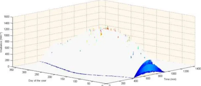
Figure -2 displays a three-dimension plot for 1-min global irradiance from the Baseline Surface Radiation Network (BSRN1) station of Payerne (Switzerland) in 2009. The intra-year as well as the intra-day trends of the time series are clearly revealed.

In the Figure -3 it has been added the envelope of the horizontal irradiance at the top of atmosphere (GHItoa), the light-grey surface. As we have mentioned above, some measured data are greater than this envelope. The distribution of these data is scattered over the year and over the time in the day, there is no structure in this data except for the sunrise and sunset hours, when the diffusion of irradiance by the atmosphere results in measured data greater than zero while the sun is under the horizon (it is seen as a blue line for very low irradiance values in the figure).

Thus, for the case of irradiance, other range limits have been proposed. The BSRN organization proposes wraparound surfaces that they are, roughly, 1.2 and 1.5 times this irradiance at the top of atmosphere, GHItoa, plus a constant, as range for rare observations limits and extrema ones, respectively (see Tables -2and -3).

Muneer and Fairooz (2002) propose as range limit 1.2 times the normal irradiance at the top of the atmosphere (corrected from Sun-Earth distance), I0, that is, without the projection on

the horizontal plane. We have compared this limit with the limits proposed by the BSRN. For the comparison we have chosen to plot a cross-sectional view of the Figure -3.

Figure -2: Three dimensional representation of 1-min average global horizontal irradiance for Payerne (Switzerland) in 2009.

1

(20)

Figure -3: The same as Figure -2 where it has been put on top the wraparound limit surface value of the horizontal irradiance on the top of atmosphere.

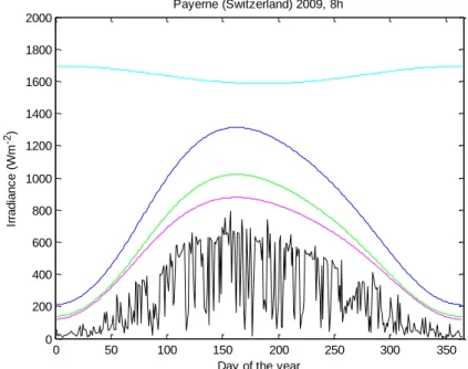
The figure -4 is this cross-sectional view for the same time of the day (8 h, UT) for all along the year, where it has been added the other range limits mentioned. This figure gives a better idea about their gap respect the measurement values, for the measurements from Payerne, at 8 h (UT) during the year 2009.

As we can see in this figure, the limit proposed by Muneer (light-blue line) is a physical version of the limit proposed by the WMO, who suggest a constant limit of 1600 W m-2 for all day long and for all the days in the year (WMO, No.488).

When we plot this kind of graph for midday, again all along the year (Figure -5), we can see that the gap between measured data and the BSRN limit based on extrema is too large, larger than the limit proposed by Muneer based on the normal irradiance at the top of atmosphere I0. This is the reason why we propose, in the present report, to choose the range

limit based on extrema as the minimum between the two mentioned limits. Nevertheless, we find useful to preserve the lower limits to flag data greater than them: in this case, these data should always be verified.

Note that in the Figure -4, the normal irradiance at the top of the atmosphere is slightly greater in winter than in summer in the case of Nord Hemisphere, since the distance to Sun is smaller in winter than in summer. For the South Hemisphere this trend is the opposite, greater in summer than in winter.

(21)

Figure -4: Illustration of different range limit controls for global horizontal irradiance. Black line is the 1–min average time series. Pink line is the horizontal irradiance on top of atmosphere. Green line is the BSRN limit range based on rare observations. Blue line is the BSRN limit range based on extrema. Light blue line is the 1.2 times the normal irradiance at the top of atmosphere, range proposed by Muneer and Fairooz (2002).

Figure -5: Choice of the proposed range limit defined as the minimum between BSRN and Muneer limits based on extrema. Colour code lines are the same that in Figure -4. Solid red line is the proposed range limit for global horizontal irradiance, particularized in this Figure for the midday of all the days of 2009, in the location of Payerne (Switzerland).

With the same idea to illustrate the range limits, we show in Figure -6 the range limits proposed by the BSRN organization for normal direct irradiance, BNI. In this case, 1-min data series has been plotted, for 7 h (UT) all along the year and also for 12 h (UT). Both limits have been retained as quality control for ENDORSE project.

0 50 100 150 200 250 300 350 0 200 400 600 800 1000 1200 1400 1600 1800 2000

Day of the year

Ir ra d ia n c e ( W m -2) Payerne (Switzerland) 2009, 8h 0 50 100 150 200 250 300 350 0 200 400 600 800 1000 1200 1400 1600 1800 2000

Day in the year

Ir ra d ia n c e ( W m -2) Payerne (Switzerland) 2009, 12h

(22)

Figure -6: Range limits for normal direct irradiance for one minute data series. Blue line: normal irradiance at the top of atmosphere. Green line: BSRN range limit based on rare observations. Black line: measures from BSRN station of Payerne at 7 h (left) and 12 h (right) all along the year 2009.

Similarly, limits proposed by the BSRN organization as well as from Muneer and Fairooz (2002) for 1-min diffuse irradiance (DHI) have been plotted in Figure -7. As for global irradiance, we propose to truncate the BSRN limit based on extrema with the proposition from Muneer when the later is smaller than the former (solid red line in the Figure -7, on the right).

Figure -7: Range limits for horizontal diffuse irradiance for 1-minute average time series. Black line: measures from BSRN station of Payerne at 12h all along the year 2009. Colour code lines are the same that in Figure -4, particularized for diffuse values shown in the Tables -2 and -3.

For the hourly time average time series, care must be taken with the computation of these limits for QC of irradiance. Commonly the time associated to an hourly average data is the time at the end of the integration period, while the average is done for the whole hour. This fact has some drift effects in the sunrise and sunset time, for example. The limits should be computed for the middle of the hour and not for the end of it. Figures -8 and -9 illustrate the drift effect in limit values in relation to this matter. For morning hourly averages (Figure -8, left), limits compute at the end of the period (dotted lines) are greater than they should and, the opposite, in the afternoon (Figure -8, right), they are smaller than they should. Note that for noon values (Figure -9), there is almost no difference.

0 50 100 150 200 250 300 350 0 200 400 600 800 1000 1200 1400 1600 1800 2000

Day of the year

(23)

Figure -8: Drift effect in the computation of limits for QCPs for global hourly irradiance averages for Payerne (Switzerland) in 2009. Colour code lines are the same that in Figure -4. Solid lines are limits compute in the middle of the hour; dotted lines are limits compute in the end of the hour. On the left, for 8 h for all the days in the year; on the right, for 18 h. In the morning, limits computed at the end of the hour are greater than they should; in the afternoon are smaller than they should.

Figure -9: Same as Figure -8 but for midday. The drift effect is almost inexistent at noon.

Note that, in Table -6, for hourly average values of global irradiance there is another QCP with respect to 1-min average QCPs. For 1-min average values, the local configuration of clouds may yield in values greater than the horizontal irradiance at the top of atmosphere. For hourly average values this event is much less likely (it would mean that the cloud position relative to the Sun has been kept for several minutes, which is unlikely).

For global horizontal irradiance, for the daylight hours (that is between the sunrise and sunset times) also a minimum value has been proposed by Geiger et al. (2002). This minimum value was set up according to the analysis of the collected data and to the minima of clearness index found in the last and previous editions of the European Solar Radiation Atlas (ESRA, 2000). A global irradiance value of 0.03 times the horizontal extraterrestrial at the top of atmosphere represents a heavily overcast sky.

0 50 100 150 200 250 300 350 0 200 400 600 800 1000 1200 1400 1600 1800 2000

Day of the year

(24)

Diffuse irradiance, for daylight hours, share the same minimum than for global irradiance, due to, for overcast conditions, diffuse has nearly the same value than global irradiance, within the precision of the measurement device.

Moreover, in general, for irradiance values, for low solar elevation angles there are some refraction and diffusion effects by the atmosphere that are hardly modeled. The limits of the QCP proposed for irradiance values have been validated for different solar altitude angles, depending on the reference: Geiger et al. (2002) use solar altitudes greater than 2°; Kendrick et al. (1994) is more restrictive and use radiation data only above 4°; Younes et al. (2005) propose solar altitudes greater than 7°, which has been adopted recently for Ruiz-Arias et al. (2010). In the frame of this report, with the target of generality, we recommend also to apply the QCP for radiation values for solar altitude angles greater than 7°. The Sun covers 15° in the Sun-path every hour, so solar elevation angle greater than 7° means that the Sun is over the horizon at least thirty minutes ago, which permits for hourly averages to have a more representative value for irradiation components for the sunrise and sunset hours.

For temperature values, ranges have been selected from the WMO (WMO, No.488), which are based on the extrema records of temperature on the Earth surface. In fact, the minimum temperature recorded was achieved in Antartica2 in 1983, -89.6 °C, while the maximum value was achieved in Lybia3 in 1922, 57.8 °C.

For wind speed, when a maximum value is given, it is difficult to know exactly its meaning. Most weather agencies use the definition for sustained winds recommended by the WMO, which specifies measuring winds at a height of 10 m for 10-min average time series. However, the United States National Weather Service defines sustained winds within tropical cyclones by averaging winds over a period of one minute, measured at the same 10 m height. This is an important distinction, as the value of a 1-min sustained wind is 14 % greater than a 10-min sustained wind (Sampson et al., 1995). In the present document, we adopt the ranges recommended by WMO (WMO, No.305) for QCP based on extrema and on rare observations for WS, 2-min average time series.

Variable Unit Minimum* Maximum

GHI (W m-2) 0.03 GHItoa Min (1.2*I0,1.5*I0*cos(sza)1.2 + 100)

BNI (W m-2) 0 I0

DHI (W m-2) 0.03 GHItoa Min (0.8*I0, 0.95*I0*cos(sza)1.2 + 50)

Temp (°C) -90 60

Hum (%) 0 100

WS (m s-1) 0 150

Table -2: QCP based on extrema for sub-hourly average time series (1-min average except for WS which is 2-min average time series). SZA is the solar zenith angle. *For irradiance variables, minimum limits are for daylight time.

Variable Unit Minimum * Maximum

GHI (W m-2) 0.03 GHItoa 1.2*I0*cos(sza)1.2 + 50

BNI (W m-2) 0 0.95*I0*cos(sza)0.2 + 10

DHI (W m-2) 0.03 GHItoa 0.75*I0*cos(sza)1.2 + 30

Temp (°C) -80 50 Hum (%) 0 100 WS (m s-1) 0 80 2 http://hypertextbook.com/facts/2000/YongLiLiang.shtml 3 http://hypertextbook.com/facts/2000/MichaelLevin.shtml

(25)

Table -3: QCP based on rare observations for sub-hourly average time series (1-min average except for WS which is 2-min average time series). *For irradiance variables, minimum limits are for daylight time.

Tables -2 and -3 are extracted from Table -6, where all the QCPs for all variables used in ENDORSE and for all the average time periods are shown.

.4.6. Step QCPs

The aim of the step checks is to verify the rate of change, to detect unrealistic jumps or stagnation in values. The check is best applicable to data of high temporal resolution as the correlation between the adjacent samples increases with the sampling rate (WMO, No.488). A step check is a temporal check that uses a climatological record of how much variables can change within a certain period of time. For some variables, the limits depend on climate conditions while for others the changes may be less sensitive to local climate (Vejen et al., 2002).

Of course, the first value which will be used as a starting reference cannot be tested by this procedure. Nevertheless, if this first data has passed the other controls, it will be useful as “plausible value”, so it will be useful to be used as reference in the step control.

Sub-hourly and hourly step QCPs are extracted from WMO (No.448), Zahumensky (2004) and Vejen et al. (2002).

For wind speed, step QC for hourly data series is based on the procedure of NDBC (2009). The standard time continuity check developed at NDBC is based on variogram-based models: these variograms are defined as the expectation of square increment of a wide-sense stationarity stochastic process between two instants separated by a given time lag. For wind speed, step QC for hourly data series is based on the procedure of NDBC, 2009. The standard time continuity check developed at NDBC is based on the following expression:

(

)

T 2 1 R(T)

s = s - (Eq. -3)

where σ Τ is the standard deviation about the mean difference between measurements at a

specific time and the corresponding measurements Τ hours later, x(t+ Τ ). σ is an estimate of the standard deviation of an ensemble of measurements, and R(Τ) is the autocorrelation function of an ensemble of measurements for a time lag, Τ. Statistics were gathered for a number of stations ranging from the Gulf of Alaska to the Gulf of Mexico. It was determined that there is an approximate linear relationship between R(Τ) and Τ for values of Τ less than 12 h. Therefore, σ was recast as follows:

T c T

s = s (Eq. -4)

This is a practical representation of the general change of a normally distributed meteorological or oceanographic variable with time. NDBC has calculated c equal to 0.58 yielding the following expression:

T 58 . 0 T    (Eq. -5)

This check compares the difference between the last acceptable measurements with the current measurement, Δx, with σ Τ. If Δx is greater than σ Τ, then the measurement is flagged

and further investigation is recommended (NDBC, 2009). Sigma has an empirically value of 25 m s-1.

(26)

The underlying assumption of wide-sense stationarity is not strictly and directly applicable to all time series of meteorological data, for all time scales: Quality check derived from these variogram models should be then particularized and calibrated for each case. This is the reason why we did not consider these types of quality check for the other meteorological variables.

.4.6.1. Check on a maximum variability between two following values

The table -4 sums up the step limits for the maximum change between two following observations (WMO, No.488) for sub-hourly time series. For wind speed, the time limit is aimed at 2-min average time series:

Variable Max. Change Unit

GHI 1000 (W m-2) BNI - (W m-2) DHI - (W m-2) Temp 3 (°C) Hum 10 (%) WS 20 (m s-1)

Table -4: Maximum change between two following observations for sub-hourly average time series

.4.6.2. Check on a minimum variability within a given time interval

This is a persistence test, adequate for sub-hourly average time series, when the measurement of the variable has been done for at least 60 min. If the 1-min values do not vary over the past 60 min (for humidity, 120, as we explain below) by more than the specified limit, then the current 1-min value fails the check (Zahumensky, 2004; WMO, No.488).

The limits shown in the Table -5 come from the WMO and are applicable for the whole Earth surface (WMO, No.488).

Variable Min. Change Unit

GHI - (W m-2) BNI - (W m-2) DHI - (W m-2) Temp 0.1 (°C) Hum 0.1 (%) WS 0.5 (m s-1)

Table -5: Minimum change within 1 h for 1-min observations except for humidity which is within 2 h.

The case of relative humidity is a particular case. In this QCP we have found that the limits proposed in the references where not adequate any more. In fact, the WMO (WMO, No.488) proposition for this limit is a minimum change of 1 % in one hour. Nevertheless, after our check with data from the BSRN organization, the percentage of flagged data with this limit was more than 10 % for every year and location checked.

When a specific QCP flags a very large amount of data, this fact may be an indication that what must be revised is not this large amount of rejected data but the QCP. In this QCP we have found an issue about the improvement of quantization step of the measurement instruments. For the time when this limit was proposed by the WMO (1977) the quantization

(27)

step for humidity measurements was probably not better than 1 %. In the years after 1977 until now, technology has been improved, so the quantization step of current measurement instruments gets tenths of the unit (0.1 %). So, we propose a narrower limit for this QCP for humidity, which is expressed in the Table 4 (also in Table 5). In this sense also, we proposed this minimum change within two hours instead of only one, since we would like to propose QCP adequate for the whole geographical area of interest of ENDORSE project and it includes some areas with very stable humidity values during early hours in the day.

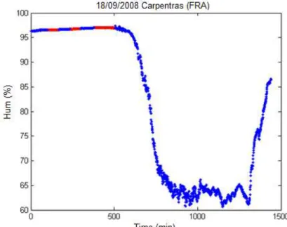
Figure -10 illustrates values that are flagged by this limit (0.1 % minimum change) when only one hour is checked, data are from the BSRN station in Carpentras (France).

Figure -10: 1-minute time series data of humidity from the BSRN station of Carpentras (France), 18/09/2008. Red data are flagged by the QCP of the minimum change within 1 h. Nevertheless, further investigations show that these data are plausible. That is the reason why this step quality control has been set within 2 h instead of only 1 h.

.4.7. Consistency QCPs

When the QCP uses two or more variables, it is named a consistency check. Both, two co-located but different variables or the same variable from two different locations may inform about the plausibility of the data. The former one is named internal consistency check; the latter one is named spatial consistency check.

.4.7.1. Internal Consistency Checks

In an internal consistency check an observation is compared with at least other co-located parameter value to see if they are physically or climatologically consistent, either instantly or for time series according to adopted observation procedures (Vejen et al., 2002).

For irradiance time series, when the three components of solar radiation are available simultaneously, the consistency check proposed by most of the references is, within an authorized bias:

GHI = BHI + DHI (Eq. -6)

where BHI is the short-wave horizontal direct irradiance at Earth Surface, computed from BNI in relation with the solar zenith angle, SZA:

(28)

There are several versions for this authorized bias: for hourly time series, Molineaux and Ineichen (2003) propose 100 W m-2 as a margin; Kendrick et al. (1994) propose 15 % of the value of GHI, for solar elevation angles greater than 4° and GHI > 20 W m-2; WMO (No.557) propose a margin of 5 % but they say that this margin is adaptable. For sub-hourly time series, BSRN (Long and Dutton, 2002) proposes this type of QCP only for GHI > 50 W m-2 and, depending on solar zenith angle, the margin allowed is 8 % or 15 % of GHI value (see Table 5). In this report we maintain the authorized bias proposed by BSRN for 1-min time series and from Kendrick et al. (1994) for hourly time series.

The authorized bias is naturally greater for hourly time series than for 1-min time series. For the calculation of BHI it is needed the SZA for the whole hour; since SZA varies in time, this calculation introduce per se a bias which is greater for hourly average than for 1-min average time series.

Note that the QCPs proposed by BSRN are defined for an interval 0° < SZA < 93°, which is larger than the interval recommended in this document, 0° < SZA < 83°. In fact, in the automated QC developed for ENDORSE, we apply the BSRN QCPs as they are defined originally, and later, we add another column in the file to flag data that corresponds to SZA between 83° and 93°: it is up to the user if he will use these data for low solar elevation angles or not.

Another internal consistency check is proposed when only two solar components are available, GHI and DHI. For hourly time series, Younes et al. (2005) and WMO (No.557) propose that DHI must be always less than or equal to GHI. On the contrary, de Miguel et al. (2001) propose that DHI may be slightly greater than GHI (10 % of the value of GHI). DHI values slightly greater than GHI are possible since normally they are not registered by the same instrument. Also, when corrections because of the shadow system is applied (shadow band correction or shadow disc correction), the correction may yields slightly greater values than the GHI ones in overcast situations. That is the reason why we proposed the last version than the other one.

For 1-min time series, the BSRN organization proposes an authorized bias, dependent on the solar altitude angle again and only for GHI > 50 W m-2, between 5 % and 10 % of GHI value (Table -6).

.4.7.2. Spatial Consistency Checks

For carrying out spatial consistency checks, it is necessary to have instantaneous data from another station sufficiently near to compare them. In these cases, more exact statistics can be applied and different kinds of data can be combined, e.g. by kriging interpolation, HIRLAM analyses, mesoscale analyses, radar and satellite data (Vejen et al., 2002). Other spatial consistency checks that can be found in the references are statistical optimal weights, fixed weights, median, simple average, Thiessen weighted average, etc.

Each pair of neighbouring observations is compared; if they agree they are both likely to be either correct or both non plausible. If they disagree, one of them is likely to be correct, the other non plausible (WMO, No.305).

MESoR project4 and IEA SHC5 Task 36 have done a survey about the interest from users by questionnaires and analysis of request of meteorological data from web sites6. In the MESoR survey, users clearly prefer time series (one or more sites) to maps (i.e. gridded values). 4 http://project.mesor.net 5 http://www.iea-shc.org/task36 6

(29)

According to IEA SHC Task 36, both types seem useful to respondents. Nevertheless, even for IEA SHC Task 36, the majority of data request are for time series and not for maps (Hoyer-Klick et al., 2010). Due to these facts, the QCPs selected for ENDORSE project are only for individual time series and no for spatial distributed data.

Table -6: QCPs for all the variables used in ENSORSE Project and all the time average periods. M o n th ly D a ily H o u rly S u b -h o u rly ( 1 -m inu te a v e ra g e e x c e p t fo r W S w h ic h is 2 -mi n u te ) GHI (Wm −2 ) QC P b a s e d o n e x tr e m a 0 .0 3 GH It o a < GH I < 1 .2 I0 QC P b a s e d o n r a re o b s e rv a tion s 0 .0 3 GH It o a < GH I < GH It o a QC P b a s e d o n e x tr e m a 0 .0 3 GH It o a < GH I < 1 .2 I0 QC P b a s e d o n r a re o b s e rv a tion s 0 .0 3 GH It o a < GH I < GH It o a QC P b a s e d o n e x tr e m a 0 .0 3 GH It o a < GH I < mi n ( 1 .2 I0 , 1 .5 I0 c o s (S ZA ) 1 .2 + 1 0 0 QC P b a s e d o n r a re o b s e rv a tion s 0 .0 3 GH It o a < GH I < 1 .2 I0 c o s (S Z A ) 1 .2 + 5 0 QC P b a s e d o n e x tr e m a 0 .0 3 GH It o a < GH I < mi n ( 1 .2 I0 ,1 .5 I0 c o s (S ZA ) 1 .2 + 1 0 0 ) QC P b a s e d o n r a re o b s e rv a tion s 0 .0 3 GH It o a < GH I < 1 .2 I0 c o s (S ZA ) 1 .2 + 5 0 S te p QC P M a x im u m s te p f o r tw o f o llo w ing mea s u re s : 1000 W m -2 BN I ( Wm −2 ) QC P b a s e d o n e x tr e m a 0 < B N I < I0 QC P b a s e d o n e x tr e m a 0 < B N I < I0 QC P b a s e d o n e x tr e m a 0 < B N I < I0 QC P b a s e d o n r a re o b s e rv a tion s 0 < B N I < 0 .9 5 I0 c o s (S Z A ) 0 .2 + 1 0 QC P b a s e d o n e x tr e m a 0 < B N I < I0 QC P b a s e d o n r a re o b s e rv a tion s 0 < B N I < 0 .9 5 I0 c o s (S Z A ) 0 .2 + 1 0 DHI (Wm −2 ) QC P b a s e d o n e x tr e m a 0 .0 3 GH It o a < DHI < 0 .8 I0 QC P b a s e d o n e x tr e m a 0 .0 3 GH It o a < DHI < 0 .8 I0 QC P b a s e d o n e x tr e m a 0 .0 3 GH It o a < D H I < m in ( 0 .8 I0 , 0 .9 5 I0 c o s (S ZA ) 1 .2 + 5 0 ) QC P b a s e d o n r a re o b s e rv a tion s 0 .0 3 GH It o a < D H I < 0 .7 5 I0 c o s (S ZA ) 1 .2 + 3 0 QC P b a s e d o n e x tr e m a 0 .0 3 GH It o a < D H I < m in ( 0 .8 I0 , 0 .9 5 I0 c o s (S ZA ) 1 .2 + 5 0 ) QC P b a s e d o n r a re o b s e rv a tion s 0 .0 3 GH It o a < D H I < 0 .7 5 I0 c o s (S ZA ) 1 .2 + 3 0 Temp ( °C) QC P b a s e d o n e x tr e m a -9 0 < Te m p < + 6 0 QC P b a s e d o n r a re o b s e rv a tion s -8 0 < Te m p < + 5 0 QC P b a s e d o n e x tr e m a -9 0 < Te m p < + 6 0 QC P b a s e d o n r a re o b s e rv a tion s -8 0 < Te m p < + 5 0 QC P b a s e d o n e x tr e m a -9 0 < Te m p < + 6 0 QC P b a s e d o n r a re o b s e rv a tion s -8 0 < Te m p < + 5 0 S te p QC P M a x im u m s te p f o r tw o f o llo w ing mea s u re s : 8 °C QC P b a s e d o n e x tr e m a -9 0 < T e m p < + 60 QC P b a s e d o n r a re o b s e rv a tion s -80 < T e m p < + 50 S te p QC P M ax im u m s te p f o r tw o f o llo w ing mea s u re s : 3 °C M inim u m s te p o v e r th e p a s t 6 0 mi n u te s : 0 .1 °C Hu m ( %) QC P b a s e d o n e x tr e m a 0 < H u m < 1 0 0 QC P b a s e d o n e x tr e m a 0 < H u m < 1 0 0 QC P b a s e d o n e x tr e m a 0 < H u m < 1 0 0 S te p QC P M a x im u m s te p f o r tw o f o llo w ing v a lue s : 3 0 % QC P b a s e d o n e x tr e m a 0 < H u m < 1 0 0 S te p QC P M a x im u m s te p f o r tw o f o llo w ing v a lue s : 1 0 % M inim u m s te p o v e r th e p a s t 1 2 0 mi n u te s : 0 .1 % WS ( m s -1 ) S te p QC P m a x im u m s te p f o r tw o f o llo w ing v a lue s : 1 5 m s -1 QC P b a s e d o n e x tr e m a ( 2 -m in a v e ra g e ) 0 < W S < 1 5 0 QC P b a s e d o n r a re o b s e rv a tion s (2 -m in a v e ra g e ) 0 < W S < 8 0 S te p QC P m a x im u m s te p f o r tw o f o llo w ing v a lue s (2 -m in a v e ra g e ): 2 0 m s -1 M inim u m s te p o v e r th e p a s t 6 0 mi n u te s e x c e p t fo r n o w ind p e riod s (1 -m in u te a v e ra g e ): 0 .5 m s -1 Co sis te nc y c he ck s D H I ≤ 1 .1 GH I D H I ≤ 1 .1 GH I For GH I > 20 W m -2(if n o t, t e s t n o t p o s s ible ) GH I / ( B H I + D H I) = 0 .1 5 DHI ≤ 1 .1 GH I For GH I > 5 0 ( if n o t, t e s t n o t p o s s ib le) : D H I/ GH I < 1 .0 5 , f o r S ZA < 7 5 ° D H I/ GH I < 1 .1 0 , f o r 9 3 ° > S ZA > 7 5 ° For D H I+BH I > 5 0 ( if n o t, t e s t n o t p o s s ible ) GH I / (B H I+D H I) ≤ 0 .0 8 , fo r S ZA < 7 5 ° GH I / (B H I+D H I) ≤ 0 .1 5, f o r 7 5 °< S ZA <9 3 °