Optical localized structures and their dynamics

HAL Id: hal-00014395

https://hal.archives-ouvertes.fr/hal-00014395

Submitted on 24 Nov 2005

HAL is a multi-disciplinary open access

archive for the deposit and dissemination of

sci-entific research documents, whether they are

pub-lished or not. The documents may come from

teaching and research institutions in France or

abroad, or from public or private research centers.

L’archive ouverte pluridisciplinaire HAL, est

destinée au dépôt et à la diffusion de documents

scientifiques de niveau recherche, publiés ou non,

émanant des établissements d’enseignement et de

recherche français ou étrangers, des laboratoires

publics ou privés.

Optical localized structures and their dynamics

Stefania Residori, Tomoyuki Nagaya, Artem Petrossian

To cite this version:

Stefania Residori, Tomoyuki Nagaya, Artem Petrossian. Optical localized structures and their

dy-namics. EPL - Europhysics Letters, European Physical Society/EDP Sciences/Società Italiana di

Fisica/IOP Publishing, 2003, 63 (4), pp.531-537. �10.1209/epl/i2003-00558-3�. �hal-00014395�

ccsd-00014395, version 1 - 24 Nov 2005

Optical localized structures and their dynamics

Institut Non Lin´eaire de Nice, UMR 6618 CNRS-UNSA, 1361 Route des lucioles, 06560 Valbonne - Sophia Antipolis;

∗ _{Department of Electrical and Electronic Engineering, Okayama University, Okayama}

700-8530, Japan

∗∗ _{Yerevan StateUniversity, 1 Manoogian Street, 375049 Yerevan, Armenia}

PACS. 42.65.Sf – Dynamics of nonlinear optical sytems; optical instabilities, optical chaos and complexity, and optical spatio-temporal dynamics.

PACS. 47.54.+r – Pattern selection; pattern formation.

Abstract. _{– When bistability and diffraction are simultaneously present, a} Liquid-Crystal-Light-Valve with optical feedback shows the appearance of localised structures. We report here new features of their dynamics, such as their appearance on successive and concentric rings and their motion along the rings. Radial and azimuthal dynamics are presented and discussed.

Introduction. – Several classes of localised structures, that we can in general consider as dissipative solitons [1], have been observed in chemistry [2] and in different areas of physics, such as in granular media [3], in binary fluid convection [4] and in surface waves experiments [5, 6]. In optics, solitary waves have been predicted to appear in bistable ring cavities [7] and localised states have been largely studied not only for their fundamental properties but also in view of their potential applications in photonics [8–11]. Sometimes named as cavity solitons, optical localised structures have been experimentally observed in photorefractifs [12], in lasers with saturable absorber [13], in Liquid-Crystal-Light-Valve (LCLV) with optical feedback [14–16], in Na vapors [17] and more recently in semiconductor microcavities [18].

A LCLV with optical feedback displays a series of bistable branches of differently oriented states. The bistability between homogenous states results from the subcritical character of the Fr´eedericksz transition, when the local electric field, which applies to the liquid crystals, depends on the liquid crystal reorientation angle [19]. In the simultaneous presence of bistabil-ity and pattern forming diffractive feedback, this system displays localised structures [14–16]. Their interactions have been recently investigated, especially as a function of the spatial fre-quency bandwidth of the system [20].

Here, new features of optical localised structures and their dynamics are presented, such as their appearance through the excitation of successive concentric rings and their destabilisation through a complex ring dynamics [21]. Azimuthal motion of the structures along the rings are observed, together with radial oscillations of the ring positions. These dynamical features suggest qualitative analogies with the behaviors theoretically predicted for solitary ring-waves, such as the azimuthal fragmentation into filaments [22] and the radial motion of solitons carrying orbital angular momentum [23].

c

2 EUROPHYSICS LETTERS

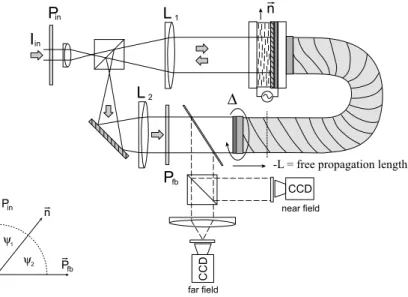
Description of the experiment. – The experimental setup is shown in Fig.1. It consists of a LCLV with optical feedback. The LCLV, as originally designed by the Akhmanov group [24], is composed of a nematic liquid crystal film sandwiched in between a glass window and a photoconductive plate over which a dielectric mirror is deposed. Coating of the bounding surfaces induces a planar anchoring (nematic director ~n parallel to the walls) of the liquid crystal film. Transparents electrodes covering the two confining plates permit the application of an electric field across the liquid crystal layer. The photoconductor behaves like a variable resistance, which decreases for increasing illumination. The feedback is obtained by sending back onto the photoconductor the light which has passed through the liquid-crystal layer and has been reflected by the dielectric mirror. This light beam experiences a phase shift which depends on the liquid crystal reorientation and, on its turn, modulates the effective voltage locally applied to the liquid crystals. Thus, a feedback is established between the liquid crystal reorientation and the local electric field.

I in L 1 L 2 P far field Pin fb P fb ψ1 ψ2 P in n n CCD

-L = free propagation length

∆

near field

CCD

Fig. 1 – The experimental setup: the LCLV is illuminated by a plane wave; the wave, reflected by the mirror of the LCLV, is sent back to the photoconductor through the optical fiber bundle. ∆ is the angle of rotation of the fiber with respect to the front side of the LCLV. ~n is the liquid crystal nematic director; Pin and Pf b are the input and feedback polarizers; L1 and L2 are two confocal 25

cm focal length lenses. −L is the free propagation length, negative with respect to the plane on which a 1:1 image of the front side of the LCLV is formed. The angles ψ1and ψ2 formed by the input and

feedback polarizers with respect to ~n are displayed in the left bottom of the figure.

The feedback loop is closed by an optical fiber bundle and is designed in such a way that diffraction and polarization interference are simultaneously present [24]. The free end of the fiber bundle is mounted on a precision rotation stage, which allows to fix a feedback rotation rotation angle ∆ with a precision of ±0.01o

. In the experiment, the fiber rotation angle is fixed to ∆ = 2π/N with N integer, whereas the optical free propagation length is fixed to L = −10 cm. At the linear stage for the pattern formation, a negative propagation distance selects the first unstable branch of the marginal stability curve, as for a focusing medium [27]. In the present case, the polarization angles of the input and feedback light beams are fixed to ψ1 = −ψ2 = 45

o

. For this parameter setting and close to the point of Fr´eedericksz transition, there is coexistence between a periodic pattern and a homogeneous solution. The

Fr´eedericksz transition point is attained for an applied voltage V0 of approximatively 3 Vrms

with a frequency of 5 kHz [19].

By increasing V0, successive branches of bistability are excited. Here, we limit our study to

the bistable branch located around V0= 18.5 Vrms. For this high value of the applied voltage,

the reoriented liquid crystal sample is similar to an homeotropic one (nematic director ~n perpendicular to the confining walls), the light feedback inducing only small reorientations around this equilibrium state. The bistable behavior here observed is very similar to the one observed close to the Fr´eedericksz transition point: the LCLV works around a point of bistability, where it may be assimilated to a phase slice with a step-like response. As pointed out recently [25], this kind of response may lead to robust localised states. Moreover, in the limit of high V0, the equilibrium state of the reoriented sample is close to saturation of the

response, that is, the nematic director is almost aligned with the applied electric field. In this highly saturated regime, the system becomes much less sensitive to external perturbations, coming from noise sources or inhomogeneities of the LCLV.

Excitation of ordered localised structures. – Fig.2 displays patterns of localised structures, as observed for an applied voltage V0= 18.45 Vrms at 5 KHz frequency. The total incident

intensity is Iin= 0.9 mW/cm2. A 50 % beam splitter is positioned before the LCLV, so that

the intensity of the feedback light beam is limited to 25 % of the total incoming intensity. This condition ensures that the LCLV works only around the switch-up point of his bistable response. The feedback rotation angle is fixed to ∆ = 2π/N with N = 6. The recurrence constraint imposed by the feedback rotation angle ∆ is very strong and leads to stationary localised structures that, once created, remains fixed to their positions.

a

b

c

d

e

f

g

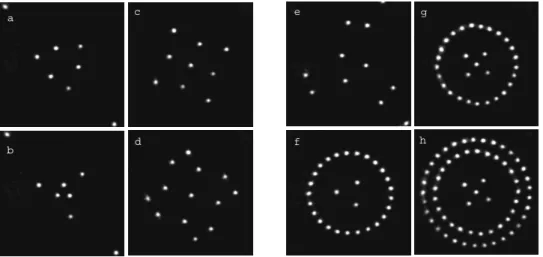
Fig. 2 – a-f) Near-field images of localised structure configurations recorded for ∆ = 2π/N with N = 6 and for different initial conditions. In g) it is displayed a typical image observed in the far-field.

Different stationary configurations may be obtained, depending on the initial condition. The resulting configurations stay stable for several minutes. If we perturb the system by blocking the feedback loop, another configuration may appear. Actually, for the parameters set in the experiment, the dark homogeneous state is also stable. Thus, once erased by blocking the feedback loop, there are no localised structures until we introduce a perturbation able to trigger their appearance. This can be done either by slightly, and temporarily, increasing V0,

4 EUROPHYSICS LETTERS

second method by using a commercial laser pointer or even a common flashlight. With the laser pointer, it is possible to adress different positions for the excitation of localised structures. Starting from a single set of N localised structures, it is possible to locally perturb the system and switch on another set in a different position or a single spot in the center.

All these manipulations prove that the observed spots are indeed localised structures, in the sense that the whole pattern is highly decomposable, that is, each structure may be considered as a single element, independent of the other structures [26]. More precisely, for the symmetry imposed by the rotation angle, the basic independent element that we have to consider here is a set of N structures, always appearing along concentric rings. The center is a singular point, that may or not be occupied by a localised structure, depending on the initial condition. a b c d e f g h

Fig. 3 – Near-field images of stationary localised structures observed for ∆ = 2π/N with a-b) N = 3 and c-d) N = 4. The structures acquire a rotation dynamics when ∆ = 2π/N + 0.1o _{with e-f) N = 3}

and g-h) N = 4.

The size of each individual spot is approximately of 500 µm, which corresponds to the basic wavelength predicted by the linear analysis for a focusing medium with a feedback mirror [27]. The distance between the spots is in average much larger than their size, which also proves that we deal with a collection of localised structures instead of a fully correlated pattern. The circular symmetry, as displayed by the appearance of the structures along concentric rings, is a consequence of the O(2) symmetry which characterizes most of optical systems and reflects the Gaussian shape of the input beam profile [22]. This last one has a transverse size of approximatel 2 cm, whereas a diaphragm before the fiber bundle selects a central active zone with a diameter of 1.2 cm.

The localisation in the near-field manifests his counterpart as a strong delocalisation in the far-field. Indeed, observations in the far-field show a diffusion of the light intensity around the central peak (zero spatial frequency). In the same time, no wavevector structure is distin-guishable. A typical far-field image is displayed in Fig.2 g, where the dashed line marks the location that would be occupied by the wavevectors of a fully correlated pattern, at the spatial frequency corresponding to the size of the individual spots. The same diffraction pattern is observed in the far-field also by changing the symmetry of the near-field distributions, as we have verified for several cases by changing ∆ = 2π/N with N = 3, 4, 5, 6, 7, 8. In Fig.3 a-b and c-d we show two typical near-field images observed for N = 3 and 4, respectively. If we

introduce a small additional rotation angle, δ = 0.1o

, in such a way that ∆ = 2π/N + δ, the structures acquire a rotation dynamics along concentric rings. Often, two adjacent rings rotate in opposite directions. Two snapshots of the dynamical rings are shown in Fig.3 e-f and g-h for N = 3 and 4, respectively. Note that similar near-field patterns, Akhseals, have been originally reported by the Akhmanov group [24]. Even though not explained in terms of localised structures, they are indeed observed in experimental conditions similar to ours.

Dynamics of localised structures. – For ∆ = 2π/N + δ, with N = 6 and δ = 0.1o

, we have set the applied voltage to V0= 18.49 Vrms(5 kHz) and we have studied the dynamics of

localised structures. For this value of V0, the structures appear spontaneously, nucleating from

the intrinsic noise in the LCLV (inhomogeneities or fluctuations). Moreover, in the vicinity of the bistability point, the slight gradients provided by the Gaussian beam profile are imposing the O(2) circular symmetry, leading to the appearance of successive and concentric rings. We expect that other shapes of the beam profile or different initial conditions would lead to different distributions of localised structures, as shown numerically in [25].

After their creation, the structures are characterized by a complex spatio-temporal dynam-ics, developing both along the radial and the azimuthal directions. The spots rotates over the rings and the ring diameter also changes during the time. Eventually, the radial motion may lead to the collapse of two adjacent rings or to the splitting of one ring into two neighboring ones. Near-field snapshots showing this dynamical behavior are displayed in Fig.4. It can be noticed that each ring reflects the underlying hexagonal symmetry, so that the number of spots is 6 on the inner ring and increases by step of 6 over two adjacent ones. However, for the outer rings, the number of spots is 17, 23, 29, that is, one spot is missing with respect to the underlying N = 6 hexagonal symmetry. In an analogous way, the number of spots for the outer rings of Fig.3f and g-h is not a multiple of the corresponding N = 3 and 4. Indeed, we find 25 instead of 24 in Fig.3f and 25, 33 instead of 24, 32 in Fig.3g-h, that is, there is one spot exceeding the expected total number of spots.

a b

d c

r θ

Fig. 4 – Near-field images of localised structures for a) to d) increasing number of rings and for ∆ = 2π/N + δ with N = 6 and δ = 0.1o_.

In Fig.5 azimuthal and radial spatio-temporal plots are reported as an example of the rings dynamics. The azimuthal (θ − t) spatio-temporal plots displayed in Fig.5 a and b show

6 EUROPHYSICS LETTERS

the rotation of the localised structures over the 12 and 17 spot rings. Note that the two rings are counter-rotating with different speed of rotation. At longer times, eventually each ring undergoes a radial instability, leading to creation and annihilation of adjacent rings. An example is shown in c) where, the fusion of two adjacent spots leads to the transition from 12 to 6 localised structures. In the azimuthal plots the radial distance is normalized to the instantaneous diameter of each ring. In d) we show a radial (r − t) spatio-temporal plot (averaged over θ), where the ring creation-annihilation may be distinguished.

0 3 6 t (sec) r

θ

θ

Fig. 5 – Azimuthal (θ −t) space-time plots for a) 12-spots and b) 17-spots ring; c) shows the transition from 12 to 6 spots. d) Radial (r − t) space-time plot showing the creation and annihilation of rings.

Finally, we show in Fig.6 the measured speed of rotation vnfor increasing number n of spots

along the successive rings. It must be recalled that the diameter of the rings is not constant during time, so that the number n is only roughly related to the distance from center. The measured data suggest that the change of rotation direction could be related to the existence of a critical radius, above which an overall phase shift changes its sign. Correspondingly, the number of spots along the outer rings becomes ”wrong”. We may argue that the overall phase shift, corresponding to the change of rotation direction, is compensated by the missing of one spot or by the appearance of one extra spot with respect to the expected multiple of N .

0 5 10 15 20 25 30 -2.0 -1.0 0.0 1.0 2.0 n v (mm/s) n

Fig. 6 – Speed of rotation for increasing number n of localized structures along the successive rings.

Conclusions. – We have shown experimental evidence of ring dynamics for optical local-ized structures. Our results are consistent with theoretical predictions for different nonlinear optical systems [22, 23], the main requirements being the bistable response of the optical system and the circular symmetry selected by the Gaussian beam profile or by diffraction.

Recently, numerical simulations for a LCLV with optical feedback have shown rings of lo-calised structures [28], in agreement with our findings. Definitive experimental observations were lacking until now, probably due to the influence of external noise and fluctuations, al-ways present in a real system. In our case, we were able to single out a regime of parameters where the response of the LCLV is closely similar to that of a binary phase slice working around the point of its saturation, so that much more insensitive to noise sources. In these conditions, we are able to control the appearance of ordered clusters of localised structures as well as the appearance of localised structures over dynamical concentric rings. All these manipulations may be useful for applications in the field of optical computing and pattern recognition. Moreover, the observed dynamics are expected to be quite general for an optical feedback system.

Acknowledgments. – This work has been supported by the ACI of the French Ministry of Research (2218 CDR 2). We gratefully acknowledge A.C. Newell for helpful discussions.

REFERENCES

[1] S. Fauve and O. Thoual, Phys. Rev. Lett. 64, 282 (1990).

[2] K-Jin Lee, W. D. McCormick, J.E. Pearson and H.L. Swinney, Nature 369, 215 (1994). [3] P.B. Umbanhowar, F. Melo and H.L. Swinney, Nature 382, 793 (1996).

[4] K. Lerman, E. Bodenschatz, D.S. Cannell and G. Ahlers, Phys. Rev. Lett. 70, 3572 (1993). [5] O. Lioubashevski, H. Arbell and J. Fineberg, Phys. Rev. Lett. 76, 3959 (1996); O. Lioubashevski,

Y. Hamiel, A. Agnon, Z. Reches and J. Fineberg, Phys. Rev. Lett. 83, 3959 (1999). [6] E. Falcon, C. Laroche and S. Fauve, Phys. Rev. Lett. 89, 204501-1 (2002).

[7] D.W. Mc Laughlin, J.V. Moloney and A.C. Newell, Phys. Rev. Lett. 51, 75 (1983). [8] G.S. McDonald and W.J. Firth, J. Opt. Soc. Am. B 10, 1081 (1993).

[9] M. Tlidi, P. Mandel and R. Lefever, Phys. Rev. Lett. 73, 640 (1994). [10] M. Brambilla, L.A. Lugiato and M. Stefani, Europhys. Lett. 34, 109 (1996). [11] W. Firth and A.J. Scroggie, Phys. Rev. Lett. 76,1623 (1996).

[12] M. Saffman, D. Montgomery and D.Z. Anderson, Opt. Lett. 19, 518 (1994). [13] V.B. Taranenko, K. Staliunas and C.O. Weiss, Phys. Rev. A 56, 1582 (1997). [14] R. Neubecker, G.L. Oppo, B. Thuering and T. Tschudi, Phys. Rev. A 52, 791 (1995). [15] P.L. Ramazza, S. Ducci, S. Boccaletti and F.T. Arecchi, J. Opt. B 2, 399 (2000). [16] Y. Iino and P. Davis, J. of Appl. Phys. 87, 8251 (2000).

[17] B. Schaepers, M. Feldmann,T. Ackemann and W. Lange, Phys. Rev. Lett. 85, 748 (2000). [18] S. Barland et al., Nature 419, 699 (2002).

[19] M.G. Clerc, S. Residori, C.S. Riera , Phys. Rev. E 63, 060701 (R), (2001).

[20] P.L. Ramazza, E. Benkler, U. Bortolozzo, S. Boccaletti, S. Ducci and F.T. Arecchi, Phys. Rev. E 65, 066204-1 (2002).

[21] S. Residori, T. Nagaya, A. Petrossian, Excitation et Dynamique des Structures Localis´es Op-tiques, proceedings of the V-th conference Rencontre du Non Lin´eaire, Paris, 13-14 March 2003. [22] J.V. Moloney, H. Adachihara, R. Indik, C. Lizarraga, R. Northcutt, D.W. McLaughlin and A.C.

Newell, J. Opt. Soc. Am. B 7, 1039 (1990).

[23] W.J. Firth and D.V. Skryabin, Phis. Rev. Lett. 79, 2450 (1997).

[24] S.A. Akhmanov, M.A. Vorontsov and V.Yu. Ivanov, JETP Lett. 47, 707 (1988); M.A. Vorontsov and W.B. Miller, in Self-Organization in Optical Systems and Applications in Information Tech-nology, edited by M.A. Vorontsov and W.B. Miller (Springer, Berlin, 1995).

[25] B.A. Samson and M.A. Vorontsov, Phys. Rev. A 56, 1621 (1997). [26] P. Coullet, C. Riera and C. Tresser, Phys. Rev. Lett. 84, 3069 (2000). [27] G. D’Alessandro and W.J. Firth, Phys. Rev. A 46, 537 (1992).

[28] P.L. Ramazza, communication at the III-rd meeting of PHASE network (European Science Fondation), Venise, 16 -19 Octobre 2002.