River network routing on the NHDPlus dataset

HAL Id: hal-00641713

https://hal.archives-ouvertes.fr/hal-00641713v2

Submitted on 18 Nov 2011

HAL is a multi-disciplinary open access

archive for the deposit and dissemination of sci-entific research documents, whether they are pub-lished or not. The documents may come from teaching and research institutions in France or

L’archive ouverte pluridisciplinaire HAL, est destinée au dépôt et à la diffusion de documents scientifiques de niveau recherche, publiés ou non, émanant des établissements d’enseignement et de recherche français ou étrangers, des laboratoires

River network routing on the NHDPlus dataset

Cédric David, David Maidment, Guo-Yue Niu, Zong-Liang Yang, Florence

Habets, Victor Eijkhout

To cite this version:

Cédric David, David Maidment, Guo-Yue Niu, Zong-Liang Yang, Florence Habets, et al.. River network routing on the NHDPlus dataset. Journal of Hydrometeorology, American Meteorological Society, 2011, 12, pp.913-934. �10.1175/2011JHM1345.1�. �hal-00641713v2�

River network routing on the NHDPlus dataset 1

Cédric H. David1,2, David R. Maidment2, Guo-Yue Niu1,3, Zong-Liang Yang1, Florence 2

Habets4 and Victor Eijkhout5 3

1. Department of Geological Sciences, Jackson School of Geosciences, University of 4

Texas at Austin, Austin, Texas, USA. 5

2. Center for Research in Water Resources, University of Texas at Austin, Austin, Texas, 6

USA. 7

3. Biosphere 2, University of Arizona, Tucson, Arizona, USA 8

4. UMR-Sisyphe 7619, CNRS, UPMC, Mines-Paristech, Paris, France. 9

5. Texas Advanced Computing Center, University of Texas at Austin, Austin, Texas, 10

USA. 11

Key words 12

RAPID, streamflow, network, matrix, parallel computing, PETSc, TAO 13

Corresponding author 14

Cédric H. David 15

Department of Geological Sciences, Jackson School of Geosciences 16

The University of Texas at Austin 17 1 University Station C1160 18 Austin, TX 78712 19 cedric.david@mail.utexas.edu 20

Abstract 21

The mapped rivers and streams of the contiguous United States are available in a 22

geographic information system (GIS) dataset called NHDPlus. This hydrographic dataset 23

has about 3 million river and water body reaches along with information on how they are 24

connected into networks. The USGS National Water Information System provides 25

stream flow observations at about 20 thousand gages located on the NHDPlus river 26

network. A river network model called RAPID is developed for the NHDPlus river 27

network whose lateral inflow to the river network is calculated by a land surface model. 28

A matrix-based version of the Muskingum method is developed herein which RAPID 29

uses to calculate flow and volume of water in all reaches of a river network with many 30

thousands of reaches, including at ungaged locations. Gages situated across river basins 31

(not only at basin outlets) are used to automatically optimize the Muskingum parameters 32

and to assess river flow computations; hence allowing the diagnosis of runoff 33

computations provided by land surface models. RAPID is applied to the Guadalupe and 34

San Antonio River Basins in Texas, where flow wave celerities are estimated at multiple 35

locations using 15-minute data and can be reproduced reasonably with RAPID. This 36

river model can be adapted for parallel computing and although the matrix method 37

initially adds a large overhead, river flow results can be obtained faster than with the 38

traditional Muskingum method when using a few processing cores, as demonstrated in a 39

synthetic study using the Upper Mississippi River Basin. 40

1. Introduction 42

Land surface models (LSMs) have been developed by the atmospheric science 43

community to provide atmospheric models with bottom boundary conditions (water and 44

energy balance) and to serve as the land base for hydrologic modeling. Over the past two 45

decades, overland and subsurface runoff calculations done by LSMs have extensively 46

been used to provide water inflow to river routing models that calculate river discharge 47

[De Roo, et al., 2003; Habets, et al., 1999a; 1999b; 1999c; 2008; Lohmann, et al., 1998a; 48

1998b; 2004; Maurer, et al., 2001; Oki, et al., 2001; Olivera, et al., 2000]. However, 49

river routing within LSMs has traditionally been done using gridded river networks that 50

best fit the computational domain used in LSMs. Today, geographic information system 51

(GIS) hydrographic datasets are increasingly becoming available at the continental scale 52

such as NHDPlus [USEPA and USGS, 2007] and the global scale such as HydroSHEDS 53

[Lehner, et al., 2006]. These datasets provide a vector-based representation of the river 54

network using the “blue line” mapped rivers and streams. Furthermore, observations of 55

the river systems are now widely available in databases such as the USGS National Water 56

Information System for the United States in which thousands of gages are available along 57

with their exact location on the NHDPlus river network. Most studies mentioned above – 58

with the exception of Habets et al. [2008] – use a limited number of gages throughout 59

large river basins, often focusing on gages located at river mouths. As the spatial and 60

temporal resolutions of weather and climate models and their underlying land surface 61

models increase, using gages located across basins would help diagnosing the quality of 62

LSM computations. The latest work on general circulation models by the international 63

scientific community, especially by the intergovernmental panel on climate change 64

[Solomon, et al., 2007], opens potential studies of the evolution of water resources with 65

global change. Using mapped streams and water bodies in LSMs could benefit the 66

resulting assessment of the impact of global change in water resources by providing 67

estimation of changes at the “blue line” level. Furthermore, the use of parallel computing 68

is quite common in regional- to global-scale atmospheric and ocean modeling, but 69

comparatively infrequent in modeling of large river networks. Generally, parallel 70

computing can be utilized to either solve problems of increasing size [as done with the 71

ParFlow model: Jones and Woodward, 2001; Kollet and Maxwell, 2006; Kollet, et al., 72

2010] or to decrease computation time [see, for example: Apostolopoulos and 73

Georgakakos, 1997; Larson, et al., 2007; Leopold, et al., 2006; von Bloh, et al., 2010].

74

These two types of approaches to parallel computing are respectively referred to as 75

scalability and speedup of calculations and the work presented herein focuses on the 76

latter. Apostolopoulos and Georgakakos [1997] investigated the speedup of streamflow 77

computations using hydrologic models in river networks as a function of network 78

decomposition and of the computing time ratio between vertical and horizontal water 79

balance calculations. Simple river routing within LSMs being traditionally performed by 80

carrying computations from upstream to downstream, one way to speedup river flow 81

modeling is to use a sequential river routing code to compute independent basins on 82

different processing cores, as done in Leopold et al. [2006] and in Larson et al. [2007]. 83

Such methods allow avoiding inter-processor communication but result in imbalanced 84

computing loads when some basins are much larger than others. Leopold et al. [2006] 85

partly addressed load imbalance by using parallel computing for surface water balance, 86

but the river routing part remains sequential. von Blow et al. [2010] implemented a 87

routing method in which computations do not have to be carried in order from upstream 88

to downstream, therefore obtaining almost perfect speedup. The work developed herein 89

investigates a way to obtain speedup while retaining traditional upstream-to-downstream 90

computations which are used in most river routing schemes. 91

The present study links a land surface model with a new river network model called 92

RAPID using NHDPlus for the representation of the river network and USGS National 93

Water Information System (NWIS) gages for the optimization of model parameters and 94

the assessment of river flow computations. All models and datasets used herein are 95

available at least for the contiguous United States. The work presented here focuses first 96

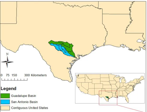
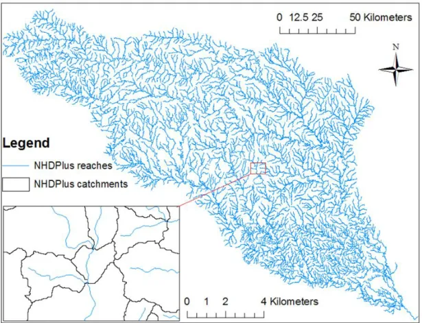
on the Guadalupe and San Antonio Basins in Texas (see Figure 1) together covering a 97

surface area of about 26,000 km2. These basins have about 5,000 river reaches and their 98

corresponding catchments in the NHDPlus dataset (see Figure 2) out of 3 million for the 99

United States. These two basins are also chosen for study because of significant 100

contributions to surface water flow from groundwater sources, because of a large 101

reservoir, at Canyon Lake, where the impacts of constructed infrastructure on flow 102

dynamics have to be considered, and because these rivers flow out into an estuarine 103

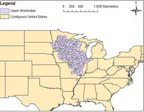
system at San Antonio Bay. A synthetic study of the performance of RAPID in a parallel 104

computing environment is also presented using the Upper Mississippi River Basin (see 105

Figure 3), which has about 180,000 river reaches in NHDPlus and covers an area of about 106

490,000 km2. 107

The research presented in this paper aims at answering the following questions: how can 108

a river model be developed for calculation of flow and volume of water in a river network 109

of thousands of “blue-line” river reaches? How can the connectivity information in 110

NHDPlus be used to run a river network model in part of the United States? How can 111

flow at ungaged locations be reconstructed? How can model computations be assessed 112

and optimized based on all available measurements? How can parallel computing be 113

used to speedup upstream-to-downstream computations of river flow within a large river 114

network? 115

First, the development of the RAPID model presented. Then, the modeling framework 116

for calculation of river flow in the Guadalupe and San Antonio River Basins using runoff 117

data from a land surface model is developed, followed by results. Finally, the speedup of 118

RAPID in a parallel computing environment is assessed. 119

2. Model development 121

The model presented here is named RAPID (Routing Application for Parallel 122

computatIon of Discharge - http://www.geo.utexas.edu/scientist/david/rapid.htm). 123

RAPID is based on the traditional Muskingum method that was first introduced by 124

McCarthy [1938] and has been extensively studied in the literature in the past 70 years. 125

The Muskingum method has two parameters, k and x , respectively a time and a 126

dimensionless parameter. Among the most noteworthy papers related to the Muskingum 127

method, Cunge [1969] showed the Muskingum method is a first-order approximation of 128

the kinematic and diffusive wave equation and proposed a method known as the 129

Muskingum-Cunge method – a second-order approximation of the kinematic and 130

diffusive wave equation – in which the Muskingum parameters are computed based on 131

mean physical characteristics of the river channel and of the flow wave. Koussis [1978] 132

proposed a variable-parameter Muskingum method based on the Muskingum-Cunge 133

method where k varies with the flow but x remains constant on the grounds that the

134

Muskingum method is relatively insensitive to this parameter. Other variable-parameter 135

Muskingum methods allow both kand x to vary [see, for example: Miller and Cunge,

136

1975; Ponce and Yevjevich, 1978], although these variable-parameter methods fail to 137

conserve mass [Ponce and Yevjevich, 1978]. Notable large-scale uses of the variable-138

parameter Muskingum-Cunge method include Orlandini and Rosso [1998] and Orlandini 139

et al. [2003]. More recently, Todini [2007] developed a mass-conservative variable-140

parameter Muskingum method known as the Muskingum-Cunge-Todini method. 141

As a first step, the traditional Muskingum method with temporally-constant parameters 142

calculated partly based on the work of Cunge [1969] is used in this study because there 143

are significant challenges to overcome in adapting the Muskingum method for river 144

networks, in efficiently running it within a parallel computing environment and in 145

developing an automated parameter estimation procedure before more sophisticated flow 146

equations are used. However, the physics of flow could be improved with many 147

variations based on the Muskingum method or adapted to the Saint Venant equations. 148

2.1 Calculation of flow and volume of water in a river network 149

In a network of thousands of reaches, matrices are needed for network connectivity and 150

flow computation. The backbone of RAPID is a vector-matrix version of the Muskingum 151

method shown in Equation (1) and derived subsequently in this section. 152 153



 



 

 

 

 

where t is time and tis the river routing time step. The bolded notation is used for

156

vectors and matrices. Iis the identity matrix. Nis the river network matrix. C₁, C and ₂ 157

3

C are parameter matrices. Q is a vector of outflows from each reach, and Qeis a vector 158

of lateral inflows for each reach. Such a vector-matrix formulation of the Muskingum 159

method has to our knowledge never been previously published. 160

Equation (1) is used for river network routing and can be solved using a linear system 161

solver. The vector-matrix notation provides one flow equation for the entire river 162

network, therefore avoiding spatial iterations. For a river network with m river reaches, 163

all vectors are of size m and all matrices are square of size m . Each element of a vector 164

corresponds to one river reach in the network. For performance purposes, all matrices are 165

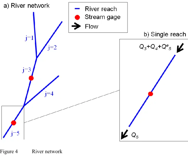
stored as sparse matrices (only the non-zero values are recorded). A five-reach, two-node 166

and two-gage river network is used here to clarify the mathematical formulation of the 167

river network model and is shown in Figure 4a). The river network is made up of a 168

combination of river reaches similar to that of Figure 4b). The model formulation is 169

presented here for a small river network but can be generalized to any size of river 170

network. 171

Q is a vector of the outflows Q_jof all reaches of the river network, where j is the index

172

of a river reach within the network: 173 174

 

 

 

 

 

 

 

Q is a vector of flows Qe_jthat are lateral inflows to the river network. Lateral inflows

177

include runoff, groundwater or any type of forced inflow (outflow at a dam, pumping, 178 etc.): 179 180

 

 

Q is provided by a land surface model, whose time step is coarser than the river routing 183

time step. Two assumptions are made in the development of RAPID, one regarding the 184

temporal variability of e

Q and one regarding the location at which Q enters the river e 185

network. In this study, the river routing time step is 15 minutes and inflow from land 186

surface runoff is available every 3 hours. In the derivation of Equation (1), e

Q is 187

assumed constant (i.e. Qe





 

188

included within a given land surface model 3-hour time step. This partial temporal 189

uniformity simplifies the river network model formulation, limits the quantity of input 190

data and facilitates the coupling with land surface models. This assumption is valid at all 191

times except at the last routing time steps before a new e

Q is made available by the land 192

surface model. Also, the external inflow e

Q is assumed to enter the network as an 193

addition to the upstream flow. With these two assumptions, the Muskingum method 194

applied to reach 5 in Figure 4b) gives the following: 195 196













 

 

 

 

 

where C , 1 C and 2 C are the Muskingum parameters that are stated in Equation (6). The 3

199

reader should note that these two assumptions are equivalent to using a unit-width lateral 200

inflow along with a term C4 as found in available literature [see, for example: Fread,

201

1993; NERC, 1975; Orlandini and Rosso, 1998; Ponce, 1986]. Equation (1) is a 202

generalization of Equation (4) using a vector-matrix notation. 203

Nis a network connectivity matrix. Berge [1958] proposed the concept of matrices

204

associated with graphs. This concept can be applied to the river network in Figure 4a)in 205

order to create the network matrix N given in Equation (5) in both full and sparse

206

formats. The network connectivity matrix is a square matrix whose dimension is the total 207

number of reaches in the network. A value of one is used at row i and column j if reach 208

j flows into reach i and zero is used everywhere else.

209 210 0 0 0 0 0 0 0 0 0 0 1 1 0 0 0 1 1 0 0 0 0 0 0 0 1 1 0 1 1                                   N (5) 211 212

The upstream inflow to the network can therefore be computed by multiplying the 213

network connectivity matrix Nby the vector of outflows Q . In case of a divergence in

214

the river network (when going downstream) or in case of a loop, a unique reach (the 215

major divergence) is used to carry all the upstream flow and the other reaches (minor 216

divergences) carry only the flow that results from their lateral inflow. This formulation 217

could be modified to take into account given fractions of flows that separate into different 218

parts of a divergence if that information is available. 219

1

C , C and ₂ C are diagonal matrices with their diagonal elements being the coefficients ₃ 220

used in the Muskingum method [McCarthy, 1938], respectively C1 j, C2 jand C3 jsuch

221

that: 222

223

















where kjis a storage constant (with dimension of a time) and xj a dimensionless

226

weighting factor characterizing the relative influence of the inflow and the outflow on the 227

volume of the reach j . The Muskingum method is stable for any x[0, 0.5], regardless

228

of the value of k and t[Cunge, 1969]. For any j : C1jC2jC3j 1.

229

In RAPID, the parameters k and x of the Muskingum method are allowed to differ from 230

one river reach to another, and corresponding vectors are defined in Equation (7): 231 232 [1, ] , [1, ] j _{j m} j _{j m} k x       _{ } _{ } k x (7) 233 234

The constants defined in Equation (6) are used as the diagonal elements of the matrices 235

1

C , C and ₂ C . Equation (8) shows an example for ₃ C₁. C and ₂ C are treated similarly. ₃ 236 237 1 2 3 4 5 1 1 1 1 1 C C C C C                    1 C (8) 238

239

The sum C1C2C equals the identity matrix. 3

240

The calculation of the volume of water in a given reach can be needed for coupling with 241

groundwater models. Here, the first order, explicit, forward Euler method is applied to 242

the continuity equation to calculate the volume of water in each river reach of the 243

network, as shown in Equation (9) where the first, second and third terms of the right-244

hand-side are the volume of water that respectively were in the river reach, flowed into 245

the reach, and discharged from the reach: 246 247





 

 

 

 

where Vis a vector of the volume of water Vjin each river reach j :

250 251

 

 

Details on the massively-parallel implementation of the matrix-based Muskingum 254

method presented in this section, and of the automated parameter estimation presented in 255

the section below are given in Appendix A. 256

2.2 Parameter estimation 257

In order to estimate the parameters k and x to be used in RAPID, an inverse method is

258

developed. The principle of an inverse method is to optimize the parameters of a model 259

so that the outputs of the model approach observations. A cost function reflecting the 260

difference between model calculations and observations is needed to assess the quality of 261

a set of model parameters. The best set of parameters is chosen as the set that minimizes 262

the cost function, and is determined through optimization. A square-error cost function 263 is chosen: 264 265

 

 

 

 

 



where the summation is made daily. The Tin exponent is for vector transpose. to and

268

f

t are respectively the first day and last day used for the calculation of . The model

269

parameter vectors k and x are kept constant within the temporal interval [ ,t t_{o f}], and the

270

cost function is calculated several times with different sets of parameters during the 271

optimization procedure. f is a scalar that allows  to be on the order of magnitude of 272

101 which is helpful for automated optimization procedures. Q

 

273

outflow vector, calculated based on the mean of all routing time steps in a given day. 274

 

g

Q is a vector with the total number of river reaches for dimension, with the daily 275

value observed g

 

Q t corresponding to reach j where gage measurements are available,

276

and zero where no gage is available. G is a sparse diagonal matrix that allows the

dot-277

product to survive only where gages are available, so that Ghas a value of one on the

diagonal element of index j if a gage is available on reach j and zero everywhere else. 279

Using the example network given in Figure 4a), G and Qg

 

280 281

 

 

 

According to Fread [1993], x[0.1;0.3] in most streams. By analogy with the kinematic

284

wave equation, Cunge [1969] showed that the parameter kof the Muskingum method is

285

the travel time of a flow wave through a river reach. For a given river reach j of length 286

j

L where a flow wave of celerity c_jtravels, k_jis obtained by dividing the length by the

287

celerity of the wave, as shown in Equation (13): 288 289 j j j L k c  (13) 290 291

Although the routing model defined by Equation (1) allows for variability of the 292

parameters ( , )k xj j on a reach-to-reach basis, attempting to automatically estimate model

293

parameters independently for all the reaches of a basin would be a costly undertaking. 294

Therefore, the search for optimal parameters is limited to determining two multiplying 295

factors kand xsuch that:

297 , 0.1 j j k j x j L k x c       (14) 298 299

To minimize the influence of the initial guess on the optimization procedure, three 300

different initial guesses for









is kept. Therefore, the optimization procedure leads to only one optimal couple 303





304

over a given basin on the grounds that the Muskingum method is relatively insensitive to 305

this parameter [Koussis, 1978]. Some data available in NHDPlus (such as mean flow, 306

mean velocity, slope, etc.) associated with available formulations for x[for example:

307

Cunge, 1969; Orlandini and Rosso, 1998] could be used to improve the proposed

308

method. 309

3. Application 310

RAPID is designed to handle large routing problems. Given a river network and 311

connectivity information as well as lateral inflow to the river network, RAPID can run on 312

any river network. In this study, a framework for computation of river flow in the 313

Guadalupe and San Antonio River Basins is developed that uses a one-way modeling 314

framework with an atmospheric dataset, a land surface model and RAPID as the river 315

model. This section presents how the Guadalupe and San Antonio River Basins are 316

described in the NHDPlus dataset, how a land surface model is used to provide lateral 317

inflow to the river network, and how the meteorological forcing is prepared. 318

3.1. RAPID used on NHDPlus 319

There are a total of 5175 river reaches with known direction and connectivity within the 320

NHDPlus description of the Guadalupe and San Antonio river basins (as shown in Figure 321

2). These 5175 reaches have an average length of 3.00 km and the average catchment 322

defined around them is 5.11 km2 in area; all are used for this study. Details on the fields 323

used in the NHDPlus dataset including the unique identifier COMID used for all river 324

reaches and their corresponding catchments; and on how NHDPlus is used with RAPID 325

are given in Appendix B. In this study, the vector of outflows in all river reaches Q was 326

arbitrarily initialized to the uniform value of 0 m3s-1 prior to running RAPID. 327

3.2. Land surface model and coupling with RAPID 328

Within this study, the core physical model governing the one-dimensional vertical fluxes 329

of energy and moisture is the Community Noah Land Surface Model with Multi-Physics 330

Options, hereafter referred to as Noah-MP [Niu, et al., 2010]. Noah-MP offers multiple 331

options for choosing the modeling of certain physical phenomena. In this study, the soil 332

moisture factor for stomatal resistance is of “Noah type” [Niu, et al., 2010] and the runoff 333

scheme is from “SIMGM” [Niu, et al., 2007]. The soil column is 2 meter deep, below 334

which is an unconfined aquifer. In order to represent the characteristics of the structural 335

soil over the model domain, the saturated hydraulic conductivity, which is determined by 336

the soil texture data, is enlarged by factor of ten (through calibration). The soil 337

hydrology of Noah (soil moisture) is run at an hourly time step and runoff data are 338

produced every three hours. In this study, the state variables of Noah were initialized 339

through a spin-up method. 340

Noah-MP calculates the amount of water that runs off on and below the land surface. 341

This quantity is used to provide RAPID with the water inflow from outside of the river 342

network. David et al. [2009] presented a coupling technique using a hydrologically 343

enhanced version of the Noah LSM called Noah-distributed [Gochis and Chen, 2003] 344

that allows physically-based modeling of the horizontal movement of surface and 345

subsurface water from the land surface to a river reach. In interest of a simpler coupling 346

scheme, the work of David et al. [2009] has been modified. In this study, a flux coupler 347

between Noah and RAPID is developed using the catchments available in the NHDPlus 348

dataset. 349

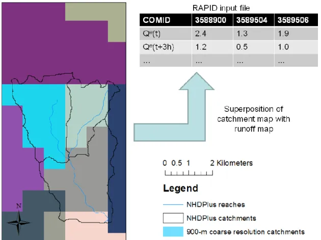
The NHDPlus catchments contributing runoff to each river reach were determined as part 350

of the NHDPlus development using a digital elevation model and its associated flow 351

accumulation and flow direction grids. These grids have a native resolution of 30 m. 352

The map of catchments is available in NHDPlus in both gridded (at 30-m resolution) and 353

vector formats in a shapefile. Running a land surface model at a 30-m resolution is very 354

resource demanding. Therefore, a coarser resolution of 900 m cell size is chosen. The 355

shapefile of NHDPlus catchment boundaries is converted to a grid of size 900 m. Within 356

this conversion process, the accuracy of the boundaries of the catchments is lowered but 357

the catchment boundaries are reasonably respected and the computational cost of the land 358

surface model calculations is reasonable. For each 3-hour output of the Noah model, 359

surface and subsurface runoff data is superimposed onto the catchment grid, and all 360

runoff that corresponds to the catchment of each river reach is summed and used as the 361

water inflow to the river reach. Figure 5 shows the principle of the flux coupler in which 362

the 900-m runoff data generated by the Noah model is superposed to the 900-m map of 363

NHDPlus catchment COMIDs to determine the lateral inflow for NHDPlus reaches used 364

by RAPID. 365

Therefore, no horizontal routing is used between the land surface and the river network in 366

the proposed scheme. This differs from some other models that use runoff from a one-367

dimensional model to force a river routing model. For instance, the two dimensional 368

wave equation is used in Gochis and Chen [2003] or the linear reservoir equation is used 369

in Ledoux et al. [1989]. 370

The coupling method used here can be adapted to any land surface model that computes 371

surface and subsurface runoff on a grid. This coupling technique is automated in a 372

Fortran program. 373

3.3. Meteorological forcing 374

Land surface models need meteorological forcing in order to compute the water and the 375

energy balance at the surface. The Noah LSM requires seven meteorological parameters: 376

precipitation, specific humidity, air temperature, air pressure, wind speed, downward 377

shortwave and downward longwave radiation. Hourly precipitation is obtained from 378

NEXRAD and downscaled from its original resolution (4.763 km) to 900 m using the 379

method developed in Guan et al. [2009]. All other meteorological parameters are 380

downloaded from the 3-hourly North American Regional Reanalysis (NARR) and 381

converted from its original resolution (32.463 km) to 900 m using a simple triangle-base 382

linear interpolation. All meteorological data are prepared for four years (01 January 2004 383

– 31 December 2007). 384

385 386

4. Calibration and results for the Guadalupe and San Antonio River Basins 387

The framework for computation of river flow that is developed in the previous section is 388

used to calculate river flow in all 5175 river reaches of the Guadalupe and San Antonio 389

River Basins for four years (01 January 2004 – 31 December 2007). In this section, flow 390

wave celerities in several sub-basins are estimated from measurements, the model 391

parameters used in RAPID are presented, and flows computed are compared to observed 392

flows. Issues related to the time step used in RAPID and to the simulated wave celerities 393

are also presented. 394

4.1. Estimation of wave celerities 395

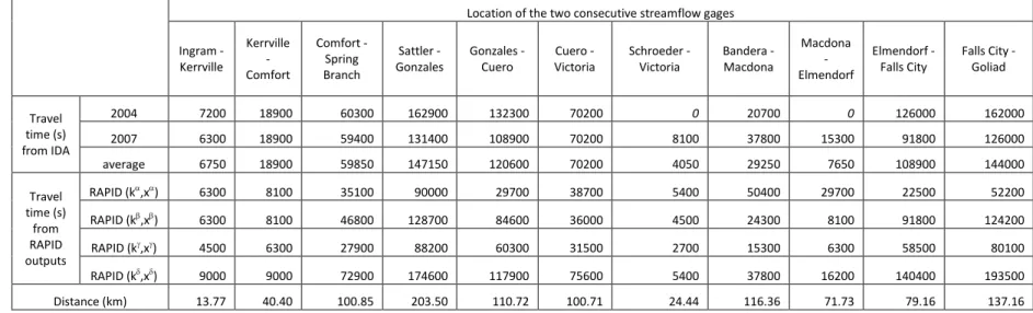
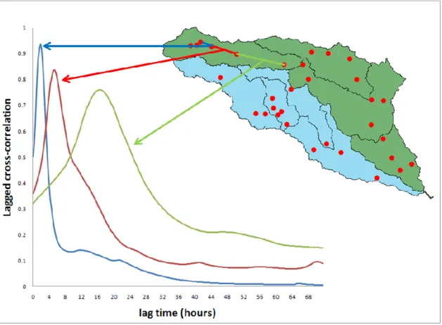
The USGS Instantaneous Data Archive (http://ida.water.usgs.gov/ida/) provides 15-396

minute flow data that can be used to determine the flow wave celerity. Data at fifteen 397

gaging stations within the two basins studied are obtained from IDA over two time 398

periods (01 January 2004 – 30 June 2004 and for 01 January 2007 – 30 June 2007). The 399

maximum lagged cross-correlation between hydrographs at two consecutive gaging 400

stations is used to determine the flow wave celerity. The lagged cross-correlation is a 401

measure of similarity between two wave forms as a function of a lag time lagapplied to

402

one of them, as shown in Equation (15). 403 404

 













 



















where a

Q and Q are the flows measured at the upstream and downstream station, b

407

respectively; and the summation is here made every 15 minutes for 6 months. Figure 6 408

shows the correlation as a function of increasing lag time between three different sets of 409

consecutive gaging stations. The lag time giving the maximum correlation is taken as the 410

travel time _travelfor the flow wave between the two stations. The travel times are 411

estimated for eleven sets of two stations and are shown on Table 1. Travel times of 0 s 412

are reported at two stations, where the flow wave is probably too fast to be captured by 413

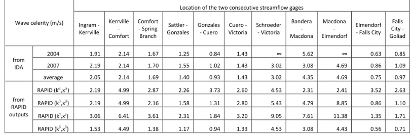
15-minute measurements. The wave celerity c is then computed using Equation (16) 414 415 travel d c   (16) 416 417

where d is the distance between two stations. The NHDPlus Flow Table Navigator Tool 418

(http://www.horizon-systems.com/nhdplus/tools.php) is used to estimate the curvilinear 419

distance between two stations along the NHDPlus river network that are shown on Table 420

1. The wave celerity has been estimated for eleven sub-basins within the Guadalupe and 421

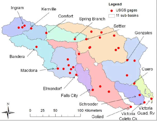
San Antonio river basins. Table 2 shows the values that are obtained for the two time 422

periods considered, as well as their average. Figure 7 shows the corresponding sub-423

basins as well as the locations of all gaging stations. 424

4.2. Parameters used in RAPID 425

RAPID needs two vectors of parameters k and xthat can either be determined using

426

physically-based equations, through optimization, or a combination of both. In this 427

study, daily stream flow data are obtained from the USGS National Water Information 428

System (http://waterdata.usgs.gov/nwis) in order to use the built-in parameter estimation. 429

Within the Guadalupe and San Antonio river basins, NWIS has 74 gages that measure 430

flow, 36 of them having full records of daily measurements the four years studied (01 431

January 2004 – 31 December 2007). These 36 stations are used for parameter estimation. 432

Four sets of model parameters – denoted by the superscripts , , and    – are used in 433

this study. These sets of parameters are all based on Equation (14) which is used with a 434

uniform wave celerity of 0 1 1

1 0.28

c  km h   m s  throughout the basin or with the

435

celerities c determined based on the IDA lagged cross-correlation study. _j

436

The first set, ( , )α α

k x is obtained from parameter estimation shown in Equation (11) using 437

the uniform wave celerity 0 1 0.28

c  m s  and the resulting values of the two multiplying

438

factors _kand _xof Equation (14) are: 439 440 0 , 0.1 0.131042 , 2.58128 j j k j x k x L k x c                 (17) 441 442 The parameters ( , )β β

k x are determined without optimization using the celerities 443

j

c determined based on the IDA lagged cross-correlation study and set to:

444 445 , 0.1 1 , 1 j j k j x j k x L k x c                 (18) 446

447

The third set of parameters ( , )γ γ

k x is obtained through optimization using the celerities 448

j

c determined based on the IDA lagged cross-correlation study and the resulting values

449 are: 450 451 , 0.1 0.617188 , 1.95898 j j k j x j k x L k x c                 (19) 452 453

The optimization converges to a value of kthat is 38% smaller than that estimated with

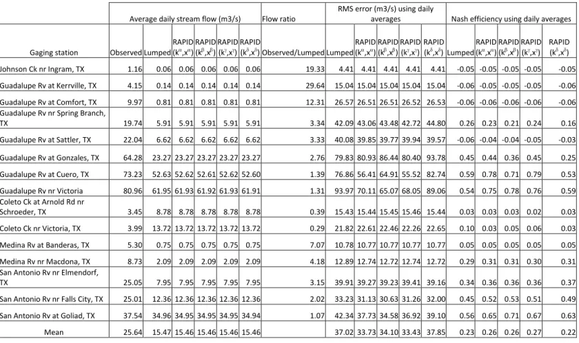
454

the IDA lagged cross-correlation, suggesting that a faster flow wave in the river network 455

produces better flow calculations. In the present study, routing on the land surface from 456

the catchment to its corresponding reach is not modeled. Therefore, one would expect 457

that the optimized flow celerity in the river network would be slower than that estimated 458

from river flow observations, which is not the case here. This suggests that runoff is 459

either produced too slowly or too far upstream of each gage; maybe because runoff in 460

land surface models is often calibrated based on a lumped value at the downstream gage 461

of a basin, as was done here with Noah-MP. Further details on the quality of runoff 462

simulations are given in Section 4.4. 463

The fourth set of parameters ( , )δ δ

k x is determined for a better match of celerity 464

calculations, as explained later in this paper. 465

4.3. Time step of RAPID simulation 466

Cunge [1969] showed that the Muskingum method is stable for any x[0, 0.5] and that

467

the wave celerity computed by the Muskingum method approaches the theoretical wave 468

celerity of the kinematic wave equation if the time step of the river routing equals the 469

travel time of the wave (for x0.5), as shown in Equation (20):

470 471 [1, ] j j L j m c t    (20) 472 473

However, both the celerity of flow and the length of river reaches vary along the network; 474

and the model formulation of RAPID allows for only one unique value of the time step 475

t

 be chosen. In the Guadalupe and San Antonio River Basins, the mean length is 3 km 476

and the median length is 2.4 km. The probability density function and the cumulative 477

density functions for the lengths of river reaches are shown in Figure 8. The celerities 478

estimated earlier are on the order of 1

2.5

c m s  . Using the median value of the reach

479

length along with 1 2.5

c m s  , Equation (20) gives  t 960s. In order to have an

480

integer conversion between the river routing time step and the land surface model time 481

step (3 hours), a value of  t 900s15minis chosen.

482

4.4. Analysis of the quality of river flow computation 483

For various model simulations, the average and the root mean square error (RMSE) of 484

computed flow rate are calculated using daily data and are given in Table 3. The Nash 485

efficiency [Nash and Sutcliffe, 1970] is bounded by the interval





estimate of the quality of modeled river flow computations when compared to 487

observations; and is also given in Table 3. An efficiency of 1 corresponds to a perfect 488

model and 0 corresponds to a model producing the mean of observations. The results 489

shown for a lumped model correspond to when runoff from Noah is accumulated at the 490

gage directly without any routing. The average values of flow in RAPID simulations are 491

tied to the amount of runoff water calculated by the Noah LSM and the bias generated by 492

the land surface model cannot be fixed by RAPID. However, the internal connectivity of 493

the NHDPlus river network is well translated in RAPID and mass is conserved within 494

RAPID since the flow rates in the lumped simulation and in all four simulations of 495

RAPID are the same. Figure 9 shows the ratio between observed and lumped stream 496

flow at 17 gages located across the Guadalupe and San Antonio River Basins. This ratio 497

is around unity downstream of the Guadalupe and San Antonio Rivers, but is greater than 498

7 upstream; suggesting that runoff is most likely overestimated at the center of the basin. 499

Additionally, runoff is largely underestimated at two stations just downstream of the 500

outcrop area of the Edwards Aquifer: the Comal River at New Braunfels and the San 501

Marcos River at San Marcos. These stations measure large average stream flow 502

(respectively 10.59 m3/s and 5.9 m3/s) although draining a relatively small area 503

(respectively 336 km2 and 129 km2), and are actually two of the largest springs in Texas. 504

These flows are much larger than the lumped runoff (respectively 0.67 m3/s and 0.26 505

m3/s), which is expected because the modeling framework presented herein does not does 506

not explicitly simulate aquifers. 507

However, the RAPID simulations ( , )α α

k x , ( , )k xβ β and ( , )k xγ γ lead to a smaller RMSE 508

and a higher Nash Efficiency than the lumped runoff. This shows that an explicit river 509

routing scheme with carefully-chosen parameters allows obtaining better stream flow 510

calculations than a simple lumped runoff scheme, as expected. 511

Within the different RAPID simulations, the set of parameters ( , )γ γ

k x gives the best 512

results for RMSE and Nash efficiency, followed by ( , )β β

k x , ( , )k xα α and ( , )k xδ δ . 513

Therefore, a greater spatial variability in the values of k contributes to the quality of 514

model results, and the built-in optimization in RAPID further enhances these model 515

results. An example hydrograph for the Guadalupe River near Victoria TX is shown in 516

Figure 10, and is computed using (k , xγ γ). 517

4.5. Comparison between estimated and computed wave celerities 518

In order to assess the capacity of the modeling framework to reproduce surface flow 519

dynamics, the celerity of the flow wave in outputs from RAPID are computed. Fifteen-520

minute river flow is computed with RAPID, and the lagged cross-correlation presented 521

earlier is used to calculate the wave celerity within the RAPID simulation. Table 2 shows 522

the celerities that are computed from RAPID outputs. In the first three sets of model 523

parameters used, the wave celerities simulated in RAPID are greater than those observed. 524

One can also notice than even for ( , )β β

k x , the model-simulated celerities are different 525

than the observed celerities which are used to determine the vector β

k itself. This was 526

predicted by Cunge [1969] who showed that the difference between the celerity of the 527

kinematic wave equation and that computed using the Muskingum method is a function 528

of both x and the quotient t L_j. Only the specific values x0.5andtverifying

529

j j

t L c

  allow obtaining the same celerity. Furthermore, the work herein is done in a 530

river network, and the celerity estimated between two points does not correspond only to 531

the main river stem but rather to a combination of all river reaches present in the network 532

in between the two points. The ratio of the average celerities from RAPID using 533

(k xβ, β)over the average observed celerities is 1.54. As a final experiment, a new set of 534

parameters ( , )δ δ

k x is created to account for the faster waves in RAPID. 535 536 , 0.1 1.54 , 1 j j k j x j k x L k x c                 (21) 537 538

Table 2 shows that the parameters ( , )δ δ

k x allow for wave celerities that are closer to the 539

observed ones than the celerities obtained with the other sets of parameters. The average 540

flow wave celerity over the 11 calculations in RAPID is within 3% of that estimated with 541

IDA flows. Unfortunately, these closer wave celerities also lead to a decrease in the 542

quality of RMSE and Nash Efficiency. Therefore, model celerities closer to celerities 543

estimated from observations can be obtained, but generally deteriorate other statistics of 544

calculations. Again, this might be due to runoff being produced too slowly or too far 545

upstream of each gage. 546

4.6 Potential improvement of spatial variability in RAPID parameters 547

In the work presented here, the parameter x is spatially and temporally constant over the 548

modeling domain and the parameter kis temporally constant but varies at the river reach

549

level based on the length of each reach and on the celerity of the flow wave going 550

through it. Flow wave celerities are estimated for 11 sub-basins based on flow 551

observations and the spatial variability of kpresented in this study is therefore partly

552

limited by the size of the sub-basins used for flow wave estimation. However such an 553

approach for computation of RAPID parameters allows taking into account wave 554

celerities that are estimated based on observations made at high temporal resolution as 555

well as verifying the modeling framework through reproduction of estimated wave 556

celerities. In a separate study applying RAPID to all rivers of Metropolitan France, 557

David et al. [2011] present a physically-based formulation ofkand a sub-basin

558

optimization for both kand x , therefore allowing further spatial variability of

559

parameters. David et al. [2011] show that using a combination of reach length, river bed 560

slope and basin residence time for the parameter kand applying the optimization

561

procedure to sub-basins both improve the efficiency and the RMSE of RAPID flow 562

computations. Such work could be adapted to the study herein based on information 563

provided in the NHDPlus dataset – for example reach length, mean annual flow velocity 564

and river bed slope – which would be advantageous when applying RAPID to domains 565

larger than the Guadalupe and San Antonio River Basins where estimation of wave 566

celerities everywhere may require excessive amounts of computations. 567

4.7 Statistical Significance 568

Changes in the routing procedure – i.e. no routing or routing using various RAPID 569

parameters – lead to various changes in the values of efficiency and RMSE, as shown in 570

Section 4.2. The statistical significance of the changes can be assessed in order to 571

determine whether or not various routing experiments are effective. For two different 572

routing procedures used, the efficiency (respectively RMSE) at one gage can be 573

compared to the efficiency (respectively RMSE) at the same gage, although variability of 574

efficiency (respectively RMSE) between independent gages can be large. Therefore, 575

there is a logical pairing of efficiency and RMSE calculated at a given gage between two 576

experiments and hence matched pair tests are appropriate to assess the statistical 577

significance. Several common options are available for matched pair tests (with 578

increasing level of complexity): the sign test, the Wilcoxon signed-ranked test [Wilcoxon, 579

1945] and the paired t-test. The sign test has no assumption on the shape of probability 580

distributions of samples used but is quite simple since only the sign of differences 581

between two paired samples is accounted for. The Wilcoxon signed-ranks test 582

incorporates the magnitude of differences between paired samples under the assumption 583

that differences between pairs are symmetrically distributed. The paired t-test may be 584

used when the differences between pairs are known to be normally distributed. The 585

assumption of the Wilcoxon signed-ranks test (symmetry) is not as restrictive as that of 586

the paired t-test (normality). In case where small sample sizes are used – as done in this 587

study – testing for symmetry or normality may not be meaningful. Additionally, 588

violations of the symmetry assumption in the Wilcoxon signed-ranks test have minimal 589

influence on the corresponding p-values [Helsel and Hirsch, 2002]. These two reasons 590

motivate the use of the Wilcoxon signed-ranks test in the study herein. The null 591

hypothesis H for this test is that the median of differences between two populations is 0

592

zero. The purpose of changes in the routing procedure being to improve results by 593

increasing the efficiency and decreasing the RMSE, alternate hypotheses can assume that 594

one population tends to be generally either larger (H ) or smaller (₁ H ) than the other. ₂

Therefore, p-values corresponding to one-sided tests are used in this study. Low 596

significance levels mean that H is unlikely, hence that a significant change is observed. 0

597

The Wilcoxon signed-ranks test sorts pairs with nonzero difference based on the absolute 598

value of the differences and sums all positive (respectively negative) ranks in a variable 599

named W(respectively W). The corresponding p-values vary with the number of

600

nonzero differences and with the value of Wand W. Fortran programs were created to

601

compute the exact value of the test statistic (not using a large-sample approximation) as 602

well as the corresponding p-values. Table 4 shows the results of the Wilcoxon signed-603

ranks test for both efficiency and RMSE and for several paired experiments using two 604

different routing procedures. The same 15 stations named on Figure 7 and used in Table 605

3 serve here for statistical significance assessment and the corresponding 15 values of 606

efficiency and of RMSE are utilized as sample values. 607

Several conclusions can be drawn from Table 4. First, the Wilcoxon signed-ranks tests 608

comparing results obtained by RAPID with parameters  , and  to a lumped runoff 609

approach show that the null hypothesis can be rejected for a one-sided test at a 10% level 610

of significance in all cases, except for the efficiency between RAPID with parameters 611

and a lumped approach at a 13% level of significance. All these tests validate that the 612

improvements mentioned in Section 4.2 (increased efficiency and decreased RMSE) are 613

statistically significant and confirm that an explicit river routing scheme allows obtaining 614

better stream flow calculations than a simple lumped runoff scheme, as expected. 615

Second, comparisons between RAPID using  and  parameters show that sub-basin 616

variability in wave celerities is advantageous to a spatially uniform wave celerity 617

approach at a 19% level of significance for efficiency and at a 7% level for RMSE. 618

Third, comparisons between RAPID using  and  parameters confirms that wave 619

celerities close to those determined from observations deteriorate results at a 3% level of 620

significance for both efficiency and RMSE. Finally, one cannot conclude on the 621

statistical significance of the comparison between RAPID using and  parameters 622

concerning the improvement of optimization procedure. However, since RAPID 623

using parameters produce better average values than RAPID using parameters and 624

since the statistical significance of RAPID using parameters compared to a lumped 625

approach is better than that of RAPID using parameters compared to lumped approach, 626

the optimization can still considered advantageous. 627

628 629

5. Synthetic study of the Upper Mississippi River Basin, speedup of parallel 630

computations 631

Through the use of mathematical and optimization libraries that run in a parallel 632

computing environment, RAPID can be applied on several processing cores. The work 633

presented above focuses on the Guadalupe and San Antonio River basins together 634

forming a river network with 5,175 river and water body reaches, which size do not 635

justify the use of parallel computing. However, all the tools and datasets used are 636

available for the Contiguous United States where the NHDPlus dataset has about 3 637

million reaches. Adapting the proposed framework to simultaneously compute flow and 638

volume of water in all mapped water bodies of the contiguous United States would 639

require solving matrix equations of size 3 million. For such a large scientific problem, 640

parallel computing can be helpful if speedup can be achieved, i.e. if increasing the 641

number of processing cores decreases the total computing time. 642

5.1 Synthetic study used for assessment of parallel performance 643

As a proof of concept, the evaluation of the parallel computing capabilities of RAPID is 644

presented here using the Upper Mississippi River Basin (shown on Figure 3) which has 645

182,240 river and water body reaches available as Region 07 in the NHDPlus dataset. 646

The number of computational elements for the Upper Mississippi River Basin is about 35 647

times larger than the combination of the Guadalupe and San Antonio River Basins, and 648

about 16 times smaller than the entire Contiguous United States. The river network of 649

the Upper Mississippi River Basin is fully interconnected, all water eventually flowing to 650

a unique outlet. 651

In order to assess the performance of RAPID, the same problem consisting in the 652

computation of river flow in all reaches of the Upper Mississippi River Basin, over 100 653

days, at a 900-second time step is solved for all results reported in Section 5.3. For this 654

performance study, the runoff data symbolized by vector e

Q in Equation (1) are 655

synthetically generated and set to 1 m3 every 3 hours for all reaches and all time steps 656

and the vectors of parameters k and x are temporally and spatially uniform as shown in 657 Equation (22): 658 659 1 , 0.3 2.5 j j j L k x m s    (22) 660 661

5.2 Basics of solving a linear system on computers 662

Numerically solving a linear system is typically an iterative process mainly involving 663

two-steps at each iteration: preconditioning followed by applying a linear solver. 664

Preconditioning is a procedure that transforms a given linear system through matrix 665

multiplication into one that is more easily solved by linear solvers, hence decreasing the 666

total number of iterations to find the solution and saving time. If the linear system is 667

triangular, preconditioning is sufficient to solve the problem, and a linear solver is not 668

needed. In a parallel computing environment, a matrix is separated into diagonal and off-669

diagonal blocks, each processing core being assigned one diagonal block and its adjacent 670

off-diagonal block. Solving a linear system in parallel is made using blocks and parallel 671

preconditioning is determined based on elements in the diagonal blocks. Preconditioning 672

is sufficient to solve a given parallel linear system if the system is diagonal by blocks – 673

i.e. all off-diagonal blocks are empty – and if each diagonal block is triangular; in most 674

other cases iterations of preconditioning and applying a linear solver are needed. 675

5.3 Parallel speedup of the synthetic study 676

For comparison purposes, the traditional Muskingum method was also implemented in 677

RAPID in order to assess the performance of the matrix-based Muskingum method 678

developed herein. Figure 11 shows a comparison of computing time between the 679

traditional Muskingum method shown in Equation (4) and applied consecutively from 680

upstream to downstream and the Matrix-based Muskingum method used in RAPID. 681

Only one processor in used for all results in Figure 11 but the computation method 682

differs. The matrix I C N being triangular (see Appendix B), solving the linear  1 683

system of Equation (1) can be limited to matrix preconditioning if using only one 684

processing core. In a parallel computing environment, I C N is separated in blocks,  1

685

each diagonal block corresponding to a sub-basin. With several processing cores, matrix 686

preconditioning would be sufficient to solve Equation (1) if I C N could be made  ₁ 687

diagonal by blocks, each diagonal block being a triangular matrix. In a river network that 688

is fully interconnected such as that of the Upper Mississippi River Basin I C N  ₁ 689

cannot be made diagonal by blocks because the connectivity between adjacent sub-basins 690

would always appear as an element in an off-diagonal block matrix (cf. Equation (23) 691

when i and j are connected but belong to different sub-basins). This limitation would 692

not apply if one was to compute the Mississippi River basin on one (or on one set of) 693

processing core(s) and the Colorado River Basin on another (or on another set of) 694

processing core(s) for example. Therefore, when solving Equation (1) on several 695

processing cores for the Upper Mississippi River Basin, preconditioning is not sufficient 696

and iterative methods need be used. An iterative method implies several computations 697

including preconditioning, matrix-vector multiplication and calculation of residual norm 698

at each iteration. 699

On one processing core, solving the matrix-based Muskingum method with 700

preconditioning only is about twice as long as solving the traditional Muskingum method, 701

as shown in Figure 11. This extra time can be explained because the computation of the 702

right-hand-side of Equation (1) is approximately as expensive as solving the traditional 703

Muskingum method and approximately as expensive as preconditioning. However, the 704

computation of the right-hand-side is done only once per time step regardless of the 705

number of iterations if using an iterative linear solver and scales very well because all 706

operations require no communication except for the product N Q which involves little  707

communication. Figure 11 also shows the computing time when using an iterative solver. 708

The sole purpose of the first iteration in an iterative solver is to determine an initial 709

residual error that is to be used as a criterion for convergence in following iterations. 710

This first iteration mainly involves preconditioning and calculation of a residual norm. 711

On one processing core only, the second iteration converges because preconditioning is 712

sufficient. The two iterations and calculations of norms explain the doubling of 713

computing time between preconditioning only and an iterative solver on one unique 714

processing core that is shown in Figure 11. Overall, the overhead created by an iterative 715

solver over the traditional Muskingum method is about a factor of four. Again, both 716

preconditioning and calculation of residual norms scale well although the latter can be 717

limited by communications. Therefore, the main issue with using a matrix method is the 718

number of iterations needed before the iterative solver converges because all other 719

overhead dissipates with an increasing number of processing cores used. Surprisingly, 720

the number of iterations needed for the iterative solver to converge increases much less 721

quickly than the number of processing cores used, hence allowing to gain total 722

computation time with increased number of processing cores and to produce results faster 723

than the traditional Muskingum method as shown on Figure 12. This suggests that even 724

in a basin where all river reaches are interdependent, some upstream and downstream 725

sub-basins can be computed separately in an iterative scheme given that they are distant 726

enough from each other. The physical explanation is that flow waves are not fast enough 727

to travel across the entire basin within one 15-minute time step. This de-coupling of 728

computations could not be achieved by using the traditional version of the Muskingum 729

method, since computations are not iterative and have to be performed going from 730

upstream to downstream. Figure 12 shows that the total computing time with an iterative 731

matrix solver on 16 processing cores is almost a third of the time needed by the 732

traditional Muskingum method and keeps decreasing further with more processing cores. 733

However, as the number of cores increase, the relative importance of the computation of 734

residual norms within the iterative solver increases up to taking almost half of the solving 735

time, as shown in Figure 12. This limitation will most likely disappear as computer 736

technology advances and communication time decreases. One should note that the output 737

files match on a byte-to-byte basis and hence model computations are strictly the same 738

regardless of the method used; i.e. traditional Muskingum method or Matrix-based 739

Muskingum method, iterative or not. This strict similarity between output files and the 740

slow increase in iterations are also verified for the study of the Guadalupe and San 741

Antonio River Basins presented above; hence the use of synthetic data and simplified 742

model parameters does not influence the trends in speedup. 743

Computing loads are balanced for all simulations in this study, i.e. the number of river 744

reaches assigned to each processing core is almost identical across cores. Figure 13 745

shows how sub-basins of the Upper Mississippi River Basin are divided among 746

processing cores as well as the longest river path of the basin. The longest path goes 747

through 8 sub-basins on 8 cores, and 14 sub-basins on 16 cores. If one were to apply the 748

traditional Muskingum method on several processing cores with the division in sub-749

basins shown in Figure 13, computations would have to be made sequentially from 750

upstream to downstream, each core having to wait for its upstream core to be done prior 751

to starting its work. Hence, assuming that the total computing time can be evenly divided 752

by the total number of nodes and neglecting communication overhead, one could only 753

hope to decrease computing time by a factor of 8 / 8 1 (no gain) for 8 cores and by a

754

factor of 16 /14 1.14 for 16 cores. The iterative matrix solver provides much better

755

results (a decrease by a factor of2.90 for 16 cores).

756

River flow is a causal phenomenon that mainly goes downstream. Therefore, when using 757

an upstream-to-downstream computation scheme and unless dealing with completely 758

separated river basins, one cannot expect to obtain perfect speedup i.e. decreasing of 759

computing time by a factor equal to the number of cores. However, today’s 760

supercomputers having tens of thousands of computing cores, one could leverage such 761

power to save human time. Additionally, the matrix method developed here can be 762

directly applied to a combination of independent river basins in which case speedup 763

would be ideally perfect. Furthermore, matrix methods such as the one developed here 764

could be adapted to more complex river flow equations – like variable-parameter 765

Muskingum methods or schemes allowing for backwater effects – in order to save total 766

computing time. Finally, the splitting up into sub-basins used here is very simple and 767

optimizing this partition by limiting connections between sub-basins or taking into 768

account flow wave celerities relatively to basin sizes could respectively help limit the 769

number of communications and the number of iterations in the linear system solver. 770