A semi-empirical model for mean wind velocity profile of landfalling hurricane boundary layers

1

A Semi-Empirical Model for Mean Wind Velocity Profile of

1

Landfalling Hurricane Boundary Layers

2

Reda Snaiki, Teng Wu

3

Department of Civil, Structural and Environmental Engineering, University at Buffalo, State University of 4

New York, Buffalo, NY 14126, USA 5

*_{Corresponding author. Email: tengwu@buffalo.edu}

6 7

Abstract: The existence of the super-gradient-wind region, where the tangential winds are larger

8

than the gradient wind, has been widely observed inside the hurricane boundary layer. Hence, the

9

extensively used log-law or power-law wind profiles under near-neutral conditions may be

10

inappropriate to characterize the boundary layer winds associated with hurricanes. Recent

11

development in the wind measurement techniques overland together with the abundance of data

12

over ocean enabled a further investigation on the boundary layer wind structure of hurricanes

13

before/after landfall. In this study, a semi-empirical model for mean wind velocity profile of

14

landfalling hurricanes has been developed based on the data from the Weather Surveillance

Radar-15

1988 Doppler (WSR-88D) network operated by the National Weather Service and the Global

16

Positioning System (GPS) dropsondes collected by the National Hurricane Center and Hurricane

17

Research Division. The proposed mathematical representation of engineering wind profile consists

18

of a logarithmic function of the height z normalized by surface roughness z0 (z z/ 0) and an empirical

19

function of z normalized by the height of maximum wind  (z/). In addition, the consideration

20

of wind direction in terms of the inflow angle is integrated in the boundary layer wind profile.

21

Field-measurement wind data for both overland and over-ocean conditions have been employed

22

to demonstrate the accuracy of simulation and convenience in use of the developed semi-empirical

23

model for mean wind velocity profile of landfalling hurricanes.

24

Keywords: Hurricanes; boundary layer; wind field; Doppler radar; Dropsondes; Landfall.

2

1. Introduction

26

Hurricane-related natural hazards are notorious for inflicting significant damage to life and

27

property through high winds, torrential rain and storm surge. The insured losses due to landfalling

28

hurricanes have been increasing due partly to the changing climate and continued escalation of

29

coastal population density (e.g., Czajkowski et al. 2011; Rappaport 2014). In general, a mature

30

hurricane consists of four main regions, namely a boundary layer, a region above the boundary

31

layer with no radial motion, an updraft region, and a quiescent eye (Carrier et al. 1971).

32

Nevertheless, the most important region for engineering applications is the boundary layer zone

33

where the dynamics and thermodynamics are usually independently examined, or weakly coupled

34

(Snaiki and Wu 2017a). The existence of the super-gradient-wind region has been widely observed

35

inside the hurricane boundary layer. The supergradient region, where the maximum wind exists,

36

was attributed by Kepert (2001) and Kepert and Wang (2001) to the strong inward advection of

37

angular momentum. While the log-law or power-law wind profiles under near-neutral conditions

38

are extensively used in engineering practice, they may be inappropriate to characterize the

39

boundary layer winds associated with mature hurricanes. Wang and Wu (2017) indicated that the

40

utilization of power-law or logarithmic profile may result in underestimation of the wind load

41

effects on tall buildings under the hurricanes. As the construction of high-rise structures continues

42

to grow in the hurricane-prone areas, it is imperative to develop a mathematical representation of

43

engineering wind profile that could take the supergradient region into account in the wind design

44

to ensure target safety and performance levels of civil infrastructures (Franklin et al. 2003; Snaiki

45

and Wu 2017a).

46

The hurricane boundary layer under marine conditions has been extensively investigated

47

due to the large database collected from reconnaissance aircraft, Stepped Frequency Microwave

3

Radiometer, moored buoy, ships data, and the Global Positioning System (GPS) dropsondes (e.g.,

49

Powell and Black 1990; Powell et al. 2003; Uhlhorn et al. 2007; Vickery et al. 2009). The National

50

Oceanic and Atmospheric Administration (NOAA) started deploying GPS dropsondes in 1997 to

51

collect dynamic and thermodynamic data from the hurricanes. The composite analysis based on

52

the GPS dropsonde data was employed by a number of researchers to inspect the vertical profile

53

of the mean wind speed inside the boundary layer region (e.g., Franklin et al. 2003; Powell et al.

54

2003; Vickery et al. 2009). Franklin et al. (2003) and Powell et al. (2003) observed the existence

55

of a supergradient region characterized by a wind maximum in the eyewall region of the hurricane

56

boundary layer. They also noted a logarithmic increase of the mean wind speed profiles from the

57

surface to the height of the supergradient region, whereas the wind speeds decrease above the

58

supergradient region due to the weakening of the horizontal pressure gradient (Franklin et al. 2003;

59

Snaiki and Wu 2017b). The studies by Kepert (2001) and Kepert and Wang (2001) indicated that

60

the height of maximum wind actually decreases with the increase of wind speed. A pronounced

61

supergradient region near the radius of maximum winds was also highlighted by Vickery et al.

62

(2009) using the GPS dropsondes data from 1997 to 2003. In addition, it was found that the lower

63

few hundred meters of the boundary layer can be well represented by the classical log-law profile.

64

Accordingly, Vickery et al. (2009) introduced a logarithmic-quadratic hurricane boundary layer

65

model for vertical mean wind speed profile, where the lower and upper altitudes are normalized

66

using the roughness length and boundary-layer height, respectively. The hurricane boundary layer

67

wind model in Vickery et al. (2009) is best suited for marine conditions. Giammanco et al. (2013)

68

also demonstrated the applicability of the log-law wind profile below the region of supergradient

69

winds by examining the data from 1997 to 2005.

4

Although the implementation of GPS dropsondes has provided a rich source of data for the

71

investigation of hurricane vertical mean wind profile, it is essentially restricted to the marine

72

conditions. The landfalling hurricane dropsonde data is scarce due to the limited inland

73

observations. The conventional approach to acquire the landfall wind data using the portable

74

towers is limited in terms of vertical coverage and hence cannot capture the supergradient region

75

(e.g., Schroeder and Smith 2003; Schroeder et al. 2009; Masters et al. 2010). The Weather

76

Surveillance Radar-1988 Doppler (WSR-88D) network operated by the National Weather Service,

77

on the other hand, offers more flexibility to thoroughly examine the hurricane wind profiles over

78

land conditions. Based on the Velocity Azimuth Display (VAD) technique (Lhermitte and Atlas

79

1961; Browning and Wexler 1968), the mean velocity is represented by a function of azimuthal

80

angle for each conical scan at a constant elevation. Giammanco et al. (2012; 2013) used the

WSR-81

88D retrieved data to examine the boundary layer vertical mean wind profile overland based on

82

the VAD method. To avoid the challenges in the determination of gradient wind speed

83

(Willoughby 1990; Powell et al. 2003; Vickery et al. 2009), Giammanco et al. (2013) used the

84

mean boundary layer (MBL) wind speed, defined as the mean wind speed averaged over a height

85

range of 10 m to 500 m according to Powell et al. (2003), to normalize the wind profiles. The wind

86

maxima below the gradient wind region was clearly identified near the radius of maximum winds.

87

In addition, the height of supergradient region was observed to increase with the radial distance

88

from storm center. To generate wind profiles for landfalling hurricanes, Krupar (2015) employed

89

a refined VAD technique to further investigated the inland data between 1995 and 2012. Roughly

90

21,000 VAD wind profiles have been constructed in Krupar (2015) based on 20 WSR-88D radars

91

distributed along the United States coastlines to comprehensively explore the vertical and

92

horizontal wind distributions inside the hurricanes. He et al. (2013), on the other hand, identified

5

the supergradient region at around 500-600m height based on the wind measurements from a

94

Doppler radar profiler and an anemometer. The existence of the supergradient winds of several

95

typhoons were also reported by Tse et al. (2014a, 2014b) utilizing measurement data taken by a

96

Doppler sodar and a boundary layer wind profiler.

97

In this study, a semi-empirical model for mean wind velocity profile of landfalling

98

hurricanes has been developed based on the data from the WSR-88D network operated by the

99

National Weather Service and the GPS dropsondes collected by the National Hurricane Center and

100

Hurricane Research Division. The collected GPS dropsonde and WSR-88D wind data were

re-101

analyzed to qualitatively and quantitatively characterize the hurricane boundary layer wind profiles

102

over the open-ocean and inland conditions. It was conjectured that the structure of hurricane

103

boundary layer winds is essentially determined by three parameters: surface shear stress w,

104

roughness length z0 and height of the maximum wind . Accordingly, the proposed mathematical

105

representation of engineering wind profile consists of a logarithmic function of the height z

106

normalized by surface roughness z0 (z z/ 0) and an empirical function of z normalized by the height

107

of maximum wind  (z/). The developed hurricane boundary layer wind profile integrates the

108

consideration of wind direction in terms of the inflow angle. The proposed semi-empirical model

109

for mean wind velocity profile of hurricanes was validated based on the observation data from

110

hurricanes Wilma and Katrina. Then, two case studies corresponding to the marine and landfalling

111

conditions, respectively, have been utilized to highlight its applicability, due to high accuracy of

112

simulation and convenience in use, to the wind design practice.

113

2. Wind Data Sources

114

2.1 GPS dropsondes

6

The GPS dropsondes, first deployed in 1997, are usually launched from an altitude of 1.5-3 km

116

with a fall speed between 10-15 m/s (Hock and Franklin 1999). The dropsonde database

117

established by the National Hurricane Center and Hurricane Research Division has provided a

118

large number of high-resolution kinematic and thermodynamic profiles. Several studies examined

119

the mean wind structure of hurricane boundary layer based on the composite profiles, where a

120

large number of GPS dropsonde data were employed (e.g., Franklin et al. 2003; Powell et al. 2003;

121

Vickery et al. 2009). Figure 1 depicts the GPS dropsonde data collected from 1996 to 2012, which

122

have been utilized in the current study. As shown in Fig. 1(a), the selected data were restricted

123

within a 300 km radius from the hurricane center to distinguish between the hurricane and

124

environmental wind profiles. In addition, the GPS dropsondes that failed to gather data below 200

125

m were excluded. A total of 2120 dropsonde measurements used here, as illustrated by Fig. 1(b),

126

are actually evenly distributed in the azimuthal direction of the hurricanes [Fig. 1(a)].

127

128

Fig. 1. GPS dropsonde data used in this study: (a) Azimuthal coverage of dropsonde data relative to hurricane

129

center; (b) Location of selected dropsondes

130

131

The composite wind profiles were generated with the 2120 collected data following the

132

approach adopted by Powell et al. (2003). The obtained profiles were then grouped according to

133 -300 -200 -100 0 100 200 300 Radius (km) -300 -200 -100 0 100 200 300 (a) Longitude (b) 90°_{W 60}°_W 0° 15°_N 30°_N 45°N 60°_N

7

the MBL wind speed of 20-29, 30-39, 40-49, 50-59, 60-69, and 70-85 m/s. These six groups were

134

ordered vertically into height bins, as illustrated in Fig. 2(a). More specifically, 10-m bins was

135

selected for heights less than 300 m, 20-m for heights between 300 m and 500 m, 50-m for heights

136

between 500 m and 1000 m, and 100-m for heights greater than 1000 m (Vickery et al. 2009).

137

Figure 2(a) indicates that the profiles exhibit a logarithmic part up to the maximum wind speed

138

(supergradient region) and its height decreases with increase of MBL wind speed (Powell et al.

139

2003; Vickery et al. 2009; Giammanco et al. 2013). The composite wind profiles were also

140

presented in terms of the storm radius r associated to dropsonde data, as depicted by Fig. 2(b). As

141

shown in the figure, the height of maximum wind generally increases with the storm radius. It is

142

noted that the averaging time of the composite wind profile obtained from the GPS dropsondes

143

can be assumed to roughly correspond to a 10-min or higher duration (Vickery et al. 2009).

144

145

Fig. 2. Composite dropsonde wind profiles grouped by: (a) MBL wind speed and (b) storm radius

146 147

2.2 WSR-88D system

148

The WSR-88D system operated by the National Weather Service is a Doppler Radar consisting of

149

several basic instruments, namely the radar product generator, the radar data acquisition and the

150 0.7 0.8 0.9 1 1.1 1.2 1.3 U/MBL 100 101 102 103 (a) MBL 20-29 m/s MBL 30-39 m/s MBL 40-49 m/s MBL 50-59 m/s MBL 60-69 m/s MBL 70-85 m/s 0.7 0.8 0.9 1 1.1 1.2 1.3 U/MBL 100 101 102 103 (b) r < 47 km 47 km ≤ r < 65 km 65 km ≤ r < 90 km 90 km ≤ r < 113 km 113 km ≤ r < 134 km 134 km ≤ r < 158 km 158 km ≤ r < 181 km 181 km ≤ r < 211 km 211 km ≤ r < 250 km 250 km ≤ r < 300 km

8

principal user processor. There are totally 155 WSR-88Ds in the United States, and the distribution

151

of WSR-88D network used in the current study is presented in Fig. 3. Weather data, such as the

152

wind speed and direction are obtained from WSR-88D based on the returned energy principle

153

where the radar receives the reflected signal first transmitted in the form of a burst energy.

154

155

Fig. 3. WSR-88D network used in this study

156 157

Krupar (2015) constructed the mean structure of landfalling hurricane boundary layer

158

winds based on the WSR-88D data from 34 hurricanes occurred from 1995 to 2012. The VAD

159

technique-based vertical wind profiles were obtained with the height bins of a 50-m resolution

160

below the 400 m, 75-m between 400 m and 700 m and 100-m above the 700 m. The VAD domain

161

in the composite analysis was restricted to those data in the range of 3-5 km from the radar site

162

(Giammanco et al. 2012; Giammanco et al. 2013; Krupar 2015). Figure 4(a) illustrates the

163

normalized composite VAD horizontal wind speed profiles grouped by MBL wind speeds.

164

Compared to Fig. 2(a) corresponding to the GPS dropsonde data, not all the obtained profiles from

165

WSR-88D data present a pronounced super-gradient-wind region. More specifically, a wind

166

maximum is observed only for wind profiles of groups 30-39 m/s and >40 m/s. Furthermore, the

167

logarithmic profiles below the wind maxima in Fig. 4(a) show a faster decay of the wind speed

168

towards the surface compared to the cases of dropsonde data. This observation suggests a more

169

significant roughness length over land than that over the marine conditions (Giammanco et al.

170 120° _W 110° W ₁₀₀°_{W 90}° W 80 ° _W 70 ° _W 30° N 40° N 50° N

9

2012). The VAD composite wind profiles were also grouped by storm radius, as depicted in Fig.

171

4(b). It is shown that the height of wind maximum increases with the storm radius. The minimum

172

value of the obtained wind maximum heights is around 550 m that is higher than the one under

173

marine conditions (Giammanco et al. 2013). It is noted that the averaging time of the VAD-derived

174

wind profiles from WSR-88D data could be assumed to be a 10-min duration (Giammanco et al.

175

2012).

176

177

Fig. 4. VAD composite WSR-88D wind profiles grouped by (a) MBL wind speed and (b) storm radius [data from

178 Krupar (2015)] 179 180 2.3 Data quality 181

The vertical profiles of wind speed were analyzed in a composite sense following the approach of

182

Powell et al. (2003) and Vickery et al. (2009). Accordingly, it can be assumed that the wind speed

183

samples are generated from a stationary process with an effective averaging time (~ 10 min)

184

corresponding to a time scale long enough to filter out the non-stationary turbulent features inside

185

the boundary layer (e.g., Powell et al. 2003; Vickery et al. 2009).

186

For the data from the GPS dropsondes, they were restricted within a 300 km radius from

187

the hurricane center to ensure the obtained mean profiles are from the hurricane winds. The

188 0.6 0.8 1 1.2 1.4 1.6 U/MBL 102 103 (a) MBL < 20 m/s MBL 20-29 m/s MBL 30-39 m/s MBL > 40 m/s 0.6 0.8 1 1.2 1.4 1.6 U/MBL 102 103 (b) r < 47 km 47 km ≤ r < 65 km 65 km ≤ r < 90 km 90 km ≤ r < 113 km 113 km ≤ r < 134 km 134 km ≤ r < 158 km 158 km ≤ r < 181 km 181 km ≤ r < 211 km 211 km ≤ r < 250 km 250 km ≤ r < 310 km 310 km ≤ r < 371 km r ≥ 371 km

10

hurricane boundary layer wind field over ocean is actually under the near-neutral conditions as

189

indicated by a number of researchers (e.g. Zhang et al. 2009), which means that the thermal effects

190

can be ignored. It should be mentioned that the collected data has been subjected to a quality

191

control by the National Hurricane Center and Hurricane Research Division to remove possible

192

errors and noises (using a 5-s low-pass filter) (Vickery et al. 2009).

193

For the data from the WSR-88D system, the VAD domain in the composite analysis was

194

restricted to those data in the range of 3-5 km from the radar site (Giammanco et al. 2012;

195

Giammanco et al. 2013; Krupar 2015). Since the thermodynamic measurements are not available

196

for the landfalling scenario through the Doppler radar, the “cut-off” approach popularly adopted

197

in the literature (e.g., Tse et al. 2013; He et al. 2016; Shu et al. 2017) was utilized here to eliminate

198

the effects of thermal instability on the wind measurements. Consequently, only the profile with a

199

MBL wind speed exceeding 10 m/s was retained in this study. Actually, the lower part of the

200

vertical wind profiles based on the collected data presents a logarithmic shape that is consistent

201

with a near-neutral stability surface layer, where the vertical distribution of momentum is

202

controlled by surface roughness (e.g., Giammanco et al. 2012; Giammanco et al. 2013).

203

3. Wind Velocity Profile

204

The wind data analyzed in Sect. 2 indicate that the large-scale wind features of hurricane boundary

205

layer may be essentially governed by three layers, namely lower part of surface friction, upper part

206

of the free atmosphere and middle part of supergradient winds. While the lower and upper parts

207

can be well described by the logarithmic solution and geostrophic wind relation, respectively, the

208

super-gradient wind mechanism needs further examination. Kepert and Wang (2001) suggested

209

that the supergradient winds may be attributed to the strong inward advection of the absolute

11

angular momentum (i.e., 2 ₂

a

M rv fr where f = Coriolis parameter and v= azimuthal wind

211

component). According to _v Ma _fr 2

r

  , a high absolute angular momentum will lead to a

212

substantial increase of the tangential wind component. The increase of the absolute angular

213

momentum is maintained through the radial advection of momentum as well as the vertical

214

diffusion and vertical advection of the radial winds. As a result, the maximum winds usually occur

215

in the eyewall region where the updraft is substantial compared to other regions (e.g., Kepert 2001;

216

Kepert and Wang 2001; Franklin et al. 2003; Powell et al. 2003). The supergradient wind actually

217

corresponds to a positive net radial force field defined as sum 1 2

p v F fv r r        (i.e., Fsum 0), 218

suggesting a higher value of the sum of Coriolis and centrifugal forces compared to the inwards

219

radial pressure gradient. The upward advection of the inward momentum weakens beyond the

220

supergradient wind region, therefore, the gradient imbalance





221

reduces the supergradient flow (Smith et al. 2009). As a result, the gradient balance





222

achieved on the top of the hurricane boundary layer. It is noted that the computationally-efficient

223

linear wind field model typically neglects the vertical advection of the radial winds (e.g., Meng et

224

al. 1995; Kepert 2001; Snaiki and Wu 2017a), hence, it usually underestimates the supergradient

225

winds. Despite a number of discussions on the mechanism of supergradient region, a close-form

226

solution for the middle-layer winds had never been done. Hence, an empirical patching between

227

the lower logarithmic-law layer and upper geostrophic-balance layer will be utilized here.

228

3.1 Wind speed

229

3.1.1 Semi-empirical wind speed profile

12

The v-momentum equation of hurricane winds from the Navier-Stokes equations will be revisited

231

to determine a general expression of the azimuthal wind component v. Accordingly, the

v-232

momentum equation can be written in the cylindrical coordinate system





233 1 v _{v v v v uv} u w fu z r r z r                 (1) 234

where





235

density; and f = Coriolis parameter. Integrating Eq. (1) from the surface to a height z leads to the

236 following: 237 0 0 1 z v z _{v v v v uv} dz u w fu dz z r r z r     _   _  _  _{ }         





Hence, the shear stress can be obtained as:

239 0 z v v w v v v v uv u w fu dz r r z r            _     _     



 = the surface shear stress in the azimuthal direction. Based on the eddy viscosity model

241

of the shear stress, _v _becomes:

242 v m dv K dz   (4) 243

where Km = the eddy viscosity. Km can be related to the frictional velocity (u*v) by using the

244

mixing-length hypothesis of Km u z*v where  is the von Karman constant. On the other hand,

245

the surface shear stress can be expressed as 2

* v

w uv

  . Therefore, Eq. (3) becomes:

246 2 * * 2 0 z v v m u u dv z _u v v v _w v uv _{fu dz} dz z K r r z r              _  _  _  _    _   



The integration of Eq. (5) leads to the following result:

13

 

The function F z  in Eq. (6) actually represents the deviation part from the logarithmic profile.

250

Since the azimuthal wind is the dominant component, similar formula of Eq. (6) will be adopted

251

here for the horizontal mean wind speed (e.g., Giammanco et al. 2013; Krupar 2015). It is expected

252

that F z  may possess two major components (terms) representing supergradient and gradient

253

wind regions and the height z of the corresponding universal forms will be normalized by the

254

height of maximum wind  and gradient wind height H, respectively. To simplify the

semi-255

empirical model of the hurricane boundary layer winds, however, the upper layer is removed in

256

the engineering formula by limiting its applicable range to the height governed by the gersotrophic

257

winds (see Sect. 3.1.2). In addition, a modified Ekman-like parametrization (product of the sine

258

and/or cosine-type function with an exponential function) (e.g., Smith 1968; Langousis et al. 2009)

259

is utilized to characterize the middle layer of supergradient winds and to empirically patch the

260

lower and upper layers. Therefore, the proposed semi-empirical wind speed profile is presented as

261 follows: 262 * 0 0 ( ) ln  sin exp       _{   }      _{ } _ _       m u z z z U z z (7) 263

where U z_m( )= mean wind speed as a function of height z;  = von Karman constant; u*= friction

264

velocity; z0= surface roughness;  = height of the maximum wind; and  = a constant determined 0

265 by the requirement of m 0 z U z _  _

 , which leads to 0 9.026. The logarithmic term of Eq. (7) can

266

be replaced by the power-law distribution for more convenient engineering applications, as

267

presented in Appendix A. The estimation of friction velocity u_* and roughness length z₀ is not

14

necessary in the empirical wind speed profile of Eq. (A.1). It should be noted that the proposed

269

wind profile of Eq. (7) or Eq. (A.1) can consider the asymmetries due to the translation speed

270

(integrated in the gradient wind) and surface roughness in the hurricane wind field distribution.

271

3.1.2 Applicable range of semi-empirical wind speed profile

272

The zero-plane displacement d, related to the average height of surface obstacles, is typically set

273

as the lower limit of the boundary layer wind model (e.g., Meng et al. 1995; Tse et al. 2013; Snaiki

274

and Wu 2017a). On the other hand, the upper limit of the developed semi-empirical wind profile

275

i

z , related to the gradient wind height, cannot be obtained straightforwardly. The wind speed at

276

gradient level is expected to decrease due to the weakening of the radial pressure gradient,

277

however, the determination of the height at which the gradient balance occurs is actually

278

challenging (e.g., Powell et al. 2003). The hurricane gradient wind height H could be between 1km

279

and 3km (e.g., Willoughby 1990; Powell et al. 2003). Based on the field-measurement data, it is

280

reasonable to assume that there is a linear overlap function between the supergradient and gradient

281

wind regions. Hence, the upper limit z_i could be determined to ensure a smooth transition between

282

these two regions. The slope associated to the semi-empirical wind profile at a starting height of

283 i z     could be computed as 1 i m z U s _z     

 _ where  is the height increment (e.g., 10 m).

284

On the other hand, the slope associated to the overlap region will be 2

_

_

( ) g m i i v U z s H z        . This 285

upper limit zi will be determined by setting s1s2, as illustrated in Fig. 5.

15 287

Fig. 5. Lower and upper limits of semi-empirical wind profile

288

3.1.3 Model fitness

289

The proposed semi-empirical hurricane boundary layer wind models of Eqs. (7) and (A.1) together

290

with the logarithmic-quadratic model of Vickery et al. (2009) were used to fit the

field-291

measurement data to represent the mean wind speed profiles. To this end, the wind data of tropical

292

cyclones Floyd (1999) on September 16, Ike (2008) on September 13 and Molave (2009) on July

293

19 (Tse et al. 2013), covering both landfall and offshore scenarios, were utilized to test the fitness

294

of these three models. The fitting results are presented in Fig. 6 and Table 1, where the

Levenberg-295

Marquardt algorithm (Levenberg, 1944; Marquardt, 1963) is employed to minimize the squared

296

difference between the observed data and numerical results. It can be seen from the fitting results

297

that the height of maximum wind  is almost identical for the profiles of Eq. (7) and Eq. (A.1),

298

both of which are less than that from Vickery’s profile. While the friction velocity u* and surface

299

roughness z₀ of the proposed semi-empirical model for Floyd, Ike, and Molave match the terrain

300

exposure conditions (Powell et al. 2004; Tse et al. 2013), Vickery’s model yielded unrealistically

301

large values.

16 303

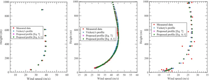
Fig. 6. Comparison between observed and fitted wind profiles for tropical cyclones Floyd (left), Ike (middle) and

304

Molave (right)

305 306

Table 1. Fitting results of mean wind speed profiles for tropical cyclones Floyd, Ike and Molave

307

308

3.2 Wind direction

309

In addition to the wind speed, the consideration of wind direction is essential in the examination

310

of wind effects on the civil infrastructures. In this study, the wind direction is considered in terms

311

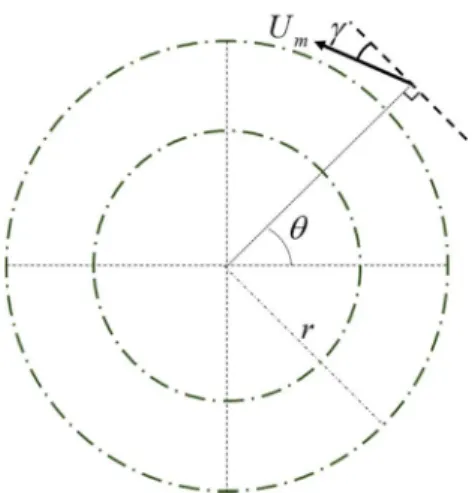
of the inflow angle  as illustrated by Fig. 7.

312 10 20 30 40 50 60 Wind speed (m/s) 0 200 400 600 800 1000 H ei gh t ( m

) Measured data_{Vickery's profile}

Proposed profile [Eq. 7] Proposed profile [Eq. A.1]

15 20 25 30 35 40 45 50 55 60 Wind speed (m/s) 0 200 400 600 800 1000 H ei gh t ( m ) Measured data Vickery's profile Proposed profile [Eq. 7] Proposed profile [Eq. A.1]

5 10 15 20 25 30 35 Wind speed (m/s) 0 200 400 600 800 1000 H ei gh t ( m ) Measured data Vickery's profile Proposed profile [Eq. 7] Proposed profile [Eq. A.1]

Tropical cyclone

Vickery’s profile Proposed profile [Eq. 7] Proposed profile [Eq. A.1]

*( / )

u m s z m 0( ) ( )m u m s *( / ) z m 0( ) ( )m U m s 10( / )  ( )m

Molave 2.01 1.85 580.41 0.99 0.15 566.57 11.03 0.14 558.53

Ike 4.11 4.13 515.84 1.83 0.38 496.34 17.53 0.16 497.01

17 313

Fig. 7. Inflow angle definition

314

From the visual inspection of the vertical profiles of inflow angle  for both marine and inland

315

conditions (e.g., Fig. 8),  decreases with increase of height. This pattern is reasonable as the

316

surface friction effects, which substantially contribute to the inflow, are wakened with height.

317

More specifically, the variation of  in the boundary layer region could be approximately

318

represented by a linear-like function of height with a various slope depending on the location inside

319

the hurricane. Therefore, it is assumed that  can be empirically expressed as:

320





where = surface inflow angle; and





322

fitting process of the measured data. To assess the goodness-of-fit, the R-squared value 2

f R (also

323

denoted as the coefficient of determination) is used in this study.

324

Two sets of constants in Eq. (8) are obtained based on the data from the dropsondes and

325

WSR-88D network, as summarized in Table 2. The obtained values of 2

f

R for the dropsondes and

326

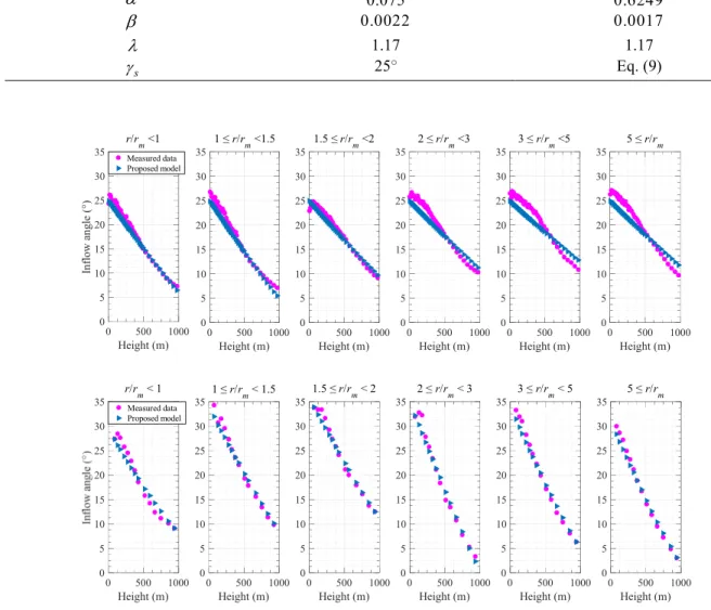
for the WSR-88D are 0.92 and 0.95, respectively. Figure 8 depicts the comparison of the measured

327

inflow angle and the fitted profiles for the marine and inland cases.

328

s

18

Table 2. Inflow angle parameters (The radius r in km)

329

Data source Dropsondes data WSR-88D data

 0.075 0.6249  0.0022 0.0017  1.17 1.17 s  25° Eq. (9) 330 331 332

Fig. 8. Comparison of measured inflow angle and fitted profiles for the marine case (upper) and inland case (lower)

333 334

Extensive studies on s for the marine conditions (e.g., Bretschneider 1972; Phadke et al. 2003;

335

Zhang and Uhlhorn 2012) indicated that the s is generally insensitive to the radial coordinate r

336

(with an average value of _s 25). For the inland conditions, however, the s significantly

337

changes with respect to r. Zilitinkevich (1989) examined the surface roughness effects on the

338

surface inflow angle for the case of a non-hurricane climate in terms of the surface Rossby number.

339

Meng et al. (1996) extended the study of Zilitinkevich (1989) to the typhoon scenarios by

340

introducing an additional non-dimensional parameter characterizing the heterogeneity of the

341 0 500 1000 Height (m) 0 5 10 15 20 25 30 35 In fl ow a ng le ( °) r/r_m<1 Measured data Proposed model 0 500 1000 Height (m) 0 5 10 15 20 25 30 35 1 ≤ r/r_m<1.5 0 500 1000 Height (m) 0 5 10 15 20 25 30 35 1.5 ≤ r/r_m<2 0 500 1000 Height (m) 0 5 10 15 20 25 30 35 2 ≤ r/r_m<3 0 500 1000 Height (m) 0 5 10 15 20 25 30 35 3 ≤ r/r_m<5 0 500 1000 Height (m) 0 5 10 15 20 25 30 35 5 ≤ r/r_m 0 500 1000 Height (m) 0 5 10 15 20 25 30 35 r/r_m< 1 0 500 1000 Height (m) 0 5 10 15 20 25 30 35 1 ≤ r/rm< 1.5 0 500 1000 Height (m) 0 5 10 15 20 25 30 35 1.5 ≤ r/r_m< 2 0 500 1000 Height (m) 0 5 10 15 20 25 30 35 2 ≤ r/r_m< 3 0 500 1000 Height (m) 0 5 10 15 20 25 30 35 3 ≤ r/r_m< 5 0 500 1000 Height (m) 0 5 10 15 20 25 30 35 5 ≤ r/r_m Measured data Proposed model 

19

vorticity in the radial direction. In this study, a similar parametrization scheme of Meng et al.

342

(1996) is employed leading to the following expression:

343







    C

s A B Ros (9)

344

where the constant coefficients A, B and C obtained by fitting WSR-88D data are 15, 80 and -0.6,

345

respectively. The non-dimensional parameter  is defined as g

ag    _ (where 2 g g v _f r    and 346 g g ag v v f r r

  _   ) with g represents the absolute angular velocity and ag corresponds to the

347

vertical component of absolute vorticity of the gradient wind (Snaiki and Wu 2017b). The

348

modified surface Rossby number Ro_s is defined as

0 g s

v

Ro  _Iz , where the inertial stability I is given

349 as _{I f} 2vg _f vg vg r r r      _  _   _{ }

  . The coefficient of determination

2 f

R is 0.83 between the

350

measured data and numerical results of Eq. (9). On the other hand, a purely-empirical formula of

351

s

 can be proposed based on the inland data from the WSR-88D as:

352 3 2 m m m m m 0.3148 3.9724 14.053 21.49875 0 5.5 31 5.5 s s r r r _{r r} r r r r r    _{     }              _{     }      (10) 353

This purely-empirical formula of Eq. (10) is actually more convenient to be used since it requires

354

only the radius of maximum winds to determine the surface inflow angle. The coefficient of

355

determination between the measured data and numerical results of Eq. (10) 2

f

R is 0.95.

356

3.3 Parameter identification

357

The semi-empirical wind profile of Eq. (7) is a function of the unique independent variable z

358

(height) and three external parameters  (height of maximum wind), u_* (friction velocity) and z₀

359

g v

20

(roughness length). The values of z0 could be obtained in neutral stratification using several

360

widely-used schemes, such as classification tables (e.g., Wieringa 1992, 1993), ground-based

361

photography (e.g., Powell et al. 2004) or averages of neutrally stratified mean gust factors (Master

362

et al. 2010). In the case that z0 is given, the friction velocity u* could be estimated based on

363





 (e.g., Powell et al. 2003). Otherwise, both u_* and z₀ can be obtained through the

364

least squares fit of the measured vertical wind speed profile in the linear-logarithmic space. In

365

addition, u_* can be directly determined from its definition when accurate and reliable

366

measurements of the horizontal Reynolds stress vector are available (e.g., Weber 1999; Masters et

367

al. 2010).

368

Currently, a well-established approach to obtain the height of maximum wind in Eq. (7)

369

has not been developed yet. Kepert and Wang (2001) indicated that the linear height-resolving

370

model, although underestimates the magnitude of the supergradient winds, can be used to

371

effectively estimate the height of maximum wind. According to the linear theory, the height of

372

maximum wind is inversely proportional to the square root of the inertial stability I(e.g.,

373

Rosenthal 1962; Kepert 2001; Eliassen and Lystad 1977; Vickery et al. 2009; Snaiki and Wu

374

2017a). On the other hand, Vickery et al. (2009) claimed that the height scale can be better modeled

375

as a function of 1 I compared to that of 1 I . In addition, the contribution of surface roughness

376

corresponding to various terrain exposure conditions to the height scale should be integrated. As a

377

result, the height of maximum wind in this study is determined according to the following formula:

378

 

 

 

ln  aln I bln Ros c (11)

379

where (a b c, , ) = empirical constants. The fitting results of these constants based on the measured

380

data under the marine and inland conditions are presented in Table 3, with corresponding

21

squared values between measured and simulated heights of 0.77 and 0.87, respectively. A negative

382

value of parameter a implies that  is inversely proportional to the inertial stability, while a

383

negative value of parameter b indicates that  increases with the surface roughness. Figure 9

384

depicts the comparison of field-measured and numerically-calculated s for both marine and

385

inland cases, and good agreements are achieved.

386

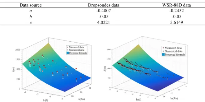
Table 3. Parameters for the height of maximum wind

387

Data source Dropsondes data WSR-88D data

a -0.4807 -0.2452

b -0.05 -0.05

c 4.0221 5.6149

388

Fig. 9. Comparison of field-measured and numerically-calculated heights of maximum wind for (left) the marine

389

case and (right) the inland case

390

3.4 Sensitivity Analysis

391

To more comprehensively examine the proposed semi-empirical model for the mean wind velocity

392

profiles of hurricanes, the sensitivity analysis of the height of maximum wind

393

 

 

 

ln  aln I bln Ros c, the surface inflow angle







C

s A B Ros

    and the inflow angle

394





   was conducted, and presented in Fig. 10. The radial variation of the inertial

395

stability I, surface Rossby number Ro_s and parameter  were determined based on the data from

396

hurricane Katrina (2005) [to be detailed in the model validation (Sect. 4.1)]. It is shown that the

22

height of maximum wind  is not sensitive to a, while b and c substantially alter its values. For

398

the inflow angle ( )z ,  and  only slightly change its slope and  marginally modifies its profile

399

concavity. On the other hand, no significant change (a maximum value of 2) in the surface angle

400

_s is observed for various values of A, B and C.

401

402

Fig. 10. Sensitivity analysis of proposed wind profile parameters

403

4. Model Validation and Application

404

4.1 Model validation

405

The developed semi-empirical model for hurricane mean wind velocity profile will be validated

406

based on two scenarios, namely hurricane Wilma (2005) and hurricane Katrina (2005).

407

Hurricane Wilma had devastating damages on Cuba, Mexico and south Florida. It reached

408

tropical Storm status on 17 October 2005 and became a hurricane on 18 October 2005. It was then

409

intensified to Category 5 hurricane on 19 October with a maximum sustained surface wind of 82.3

410 0 20 40 (°) 0 500 1000 H ei gh t ( m ) =0.5900=0.6249 =0.6500 0 20 40 (°) 0 500 1000 =0.0014 =0.0017 =0.0019 0 20 40 (°) 0 500 1000 =1.05 =1.17 =1.29 100 200 300 400 Radius (km) 0 10 20 30 40 s (° ) A=10 A=15 A=20 100 200 300 400 Radius (km) 0 10 20 30 40 s (° ) B=75 B=80 B=85 100 200 300 400 Radius (km) 0 10 20 30 40 s (° ) C=-0.58 C=-0.60 C=-0.62 100 200 300 400 Radius (km) 0 500 1000 1500 2000 ( m ) a=-0.2500 a=-0.2452 a=-0.2400 100 200 300 400 Radius (km) 0 500 1000 1500 2000 ( m ) b=-0.06 b=-0.05 b=-0.04 100 200 300 400 Radius (km) 0 500 1000 1500 2000 ( m ) c=5.5000 c=5.6149 c=5.7000

23

m/s. The recorded minimum central pressure was 882 hpa. Wilma hit the southern Florida as a

411

Category 3 hurricane. The comparison between the wind profiles, at the location of

412





413

0 0.1

z  m using the Land Use Land Cover (e.g., Powell et al. 2004), measured from the Doppler

414

radar KAMX and calculated based on the proposed semi-empirical model is depicted in Figure 11.

415

The identified friction velocity u_* is 1.82 m/s and the height of maximum wind  is 862.45 m.

416

All other parameters needed in the simulation were obtained from the HURDAT database on 24

417

October at 1200 UTC. A good agreement between observed and simulated wind speeds and inflow

418

angles is achieved.

419

420

Fig. 11. Observed and simulated wind speed (a) and inflow angle (b) of Hurricane Wilma

421

Hurricane Katrina reached the Hurricane strength on 25 August 2005 at 2100 UTC, then

422

crossed the southern Florida after making landfall near Miami at 2230 UTC. Katrina was

423

intensified again after a weakening stage on the eastern coast of Florida to reach Category 5

424

hurricane on 28 August. It made another landfall near Buras, Louisiana on 29 August as a Category

425

3 hurricane. Figure 12 presents the comparison between the wind profiles provided by the KAMX

426

Doppler radar and semi-empirical model at the location of





427

landfalling case with the estimated surface roughness z0 0.1m. The identified friction velocity u*

24

is 1.19 m/s and the height of maximum wind  is 715.20 m. All other parameters needed in the

429

simulation were obtained from the HURDAT database on August 26 at 0000 UTC. As shown in

430

the figure, an excellent agreement between the observed and simulated wind speeds is observed.

431

On the other hand, the simulated inflow angles show slight difference with the measurements.

432

433

Fig. 12. Observed and simulated wind speed (a) and inflow angle (b) of Hurricane Katrina

434 435

4.2 Application

436

Two case studies corresponding to the overland and marine conditions, respectively, will be

437

presented to highlight the simulation convenience and efficiency of the developed semi-empirical

438

wind model. The hurricane parameters of these two scenarios for the wind field simulation are

439

summarized in Table 4. The values of central pressure p_c, radius of maximum winds r_m, Holland

440

B parameter, translational speed c, approach angle  , and latitude and longitude





441

are utilized to obtain the gradient wind, and then the gradient-to-surface wind reduction factors

442

could be employed to derive the surface wind speed U₁₀ for the estimation of the friction velocity

443

*

u (e.g., Sparks and Huang 1999; Lee and Rosowsky 2007). With the values of z₀ listed on Table

444

4 and  obtained using Eq. (11), the wind speed and direction can be obtained based on the

25

proposed formulas of Eq. (7) and Eq. (8), respectively. The simulation results under the inland and

446

marine conditions are illustrated in Fig. 13 and 14, respectively.

447

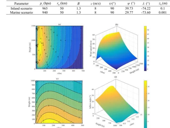
Table 4. Hurricane parameters for wind field simulation

448 Parameter p (hpa) c r (km) m B c(m/s) (°)  (°)  (°) z (m) 0 Inland scenario 965 50 1.3 8 90 39.73 -74.22 0.1 Marine scenario 940 50 1.3 8 90 29.77 -73.60 0.001 449 450 451

Fig. 13. Wind field simulation of inland scenario: (a) Contour of vertical wind speed; (b) Three dimensional shaded

452

surface of wind speed; (c) Contour of inflow angle; (d) Three dimensional shaded surface of inflow angle

453 454 (a) 4 8 8 8 8 12 12 12 12 12 12 16 16 16 16 16 16 20 20 20 20 20 20 24 24 24 24 24 24 28 28 28 28 28 28 32 32 32 32 32 32 36 36 36 36 36 40 40 40 40 40 44 44 44 44 44 48 48 48 48 48 52 52 52 100 200 300 400 500 r(km) 0 500 1000 1500 H ei gh t ( m ) rmax 0 0 5 5 5 5 10 10 10 10 15 15 15 15 20 20 20 20 25 25 25 30 ₃₀ 100 200 300 400 500 r(km) 0 100 200 300 400 500 600 700 800 900 1000 H ei gh t ( m ) (c) (a) 10 15 15 15 15 15 15 20 20 20 20 20 20 25 25 25 25 25 25 30 30 30 30 30 30 35 35 35 35 35 35 40 40 40 40 40 40 45 45 45 45 45 45 ₅₀ 50 50 50 50 50 55 55 55 55 55 60 60 60 60 60 65 65 65 65 70 100 200 300 400 500 r(km) 0 500 1000 1500 H ei gh t ( m ) r_max

26 455

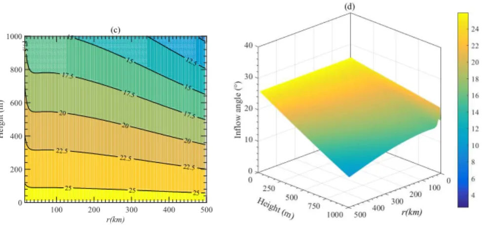
Fig. 14. Wind field simulation of marine scenario: (a) Contour of vertical wind speed; (b) Three dimensional shaded

456

surface of wind speed; (c) Contour of inflow angle; (d) Three dimensional shaded surface of inflow angle

457 458

As shown in both Figs. 13 and 14, the supergradient region is clearly identified near the

459

radius of maximum wind r_m while a log-like wind profile is obvious in the outer vortex region.

460

The comparison between the landfalling and marine cases indicates that the height of maximum

461

wind over ocean is lower than that over land. To more clearly present the abovementioned

462

observations in Figs. 13 and 14, two wind profiles corresponding to the eye-wall (r = 50 km) and

463

outer vortex regions (r = 200 km) were plotted in Fig. 15 for both inland and marine simulations.

464

The existence of the super-gradient-wind region is highlighted inside the eyewall region. In

465

addition, the height of maximum wind over ocean is around 460 m while the one over land is

466 around 680 m. 467 (c) 12.5 15 15 15 17_.5 17.5 17.5 17.5 20 20 20 22.5 22.5 22.5 25 ₂₅ 25 100 200 300 400 500 r(km) 0 200 400 600 800 1000 H ei gh t ( m )

27

468

Fig. 15. Vertical wind profile of eyewall and outer vortex regions under (a) landfall condition; (b) marine condition

469

5. Concluding Remarks

470

A semi-empirical model for mean wind velocity profile of landfalling hurricanes has been

471

developed based on the re-analysis of data from the Weather Surveillance Radar-1988 Doppler

472

(WSR-88D) network and the Global Positioning System (GPS) dropsondes. The new

473

mathematical representation of hurricane boundary layer wind profile consists of a logarithmic

474

function of the height z normalized by surface roughness z0 (z z/ 0) and an empirical function of z

475

normalized by the height of maximum wind  (z/). The proposed engineering model for the

476

height of maximum wind  highlights the contribution from both the inertial stability and surface

477

roughness. The fast and reliable estimation of  facilitates the accuracy of simulation and

478

convenience in use of the semi-empirical wind model. The consideration of wind direction in terms

479

of the inflow angle further improves the applicability of the developed hurricane wind field model

480

to the wind design practice. The new model may have a contribution to codification of the

481

landfalling hurricane boundary layer wind field, especially in the consideration of

super-gradient-482 wind region. 483 H ei gh t ( m ) H ei gh t ( m )

28

Acknowledgments

484

The support for this project provided by the NSF Grant # CMMI 15-37431 is gratefully

485

acknowledged.

486

Appendix A

487

An empirical wind speed profile could be obtained by replacing the logarithmic term of Eq. (7)

488

with the power-law distribution:

489 10 1 ( ) sin exp 10     _{     }  _{ }  _{  } _           z z z U z U (A.1) 490

where  = power law exponent; and the parameter 1 is determined by setting 0

z U z   _  491

resulting in the following expression:

492

 

Bretschneider, C.L., 1972, January. A non-dimensional stationary hurricane wave model. In Offshore Technology

495

Conference. Offshore Technology Conference.

496

Browning, K.A. and Wexler, R., 1968. The determination of kinematic properties of a wind field using Doppler radar.

497

Journal of Applied Meteorology, 7(1), pp.105-113.

498

Carrier, G.F., Hammond, A.L. and George, O.D., 1971. A model of the mature hurricane. Journal of Fluid Mechanics,

499

47(1), pp.145-170.

500

Czajkowski, J., Simmons, K. and Sutter, D., 2011. An analysis of coastal and inland fatalities in landfalling US

501

hurricanes. Natural hazards, 59(3), pp.1513-1531.

502

Eliassen, A. and Lystad, M., 1977. The Ekman layer of a circular vortex-A numerical and theoretical study.

503

Geophysica Norvegica, 31, pp.1-16.

504

Franklin, J.L., Black, M.L. and Valde, K., 2003. GPS dropwindsonde wind profiles in hurricanes and their operational

505

implications. Weather and Forecasting, 18(1), pp.32-44.

506

Giammanco, I.M., Schroeder, J.L. and Powell, M.D., 2012. Observed characteristics of tropical cyclone vertical wind

507

profiles. Wind and Structures, 15(1), p.65.

29

Giammanco, I.M., Schroeder, J.L. and Powell, M.D., 2013. GPS dropwindsonde and WSR-88D observations of

509

tropical cyclone vertical wind profiles and their characteristics. Weather and Forecasting, 28(1), pp.77-99.

510

He, Y.C., Chan, P.W. and Li, Q.S., 2013. Wind profiles of tropical cyclones as observed by Doppler wind profiler and

511

anemometer. Wind and Structures, 17(4), pp.419-433.

512

He, Y.C., Chan, P.W. and Li, Q.S., 2016. Observations of vertical wind profiles of tropical cyclones at coastal areas.

513

Journal of Wind Engineering and Industrial Aerodynamics, 152, pp.1-14.

514

Hock, T.F. and Franklin, J.L., 1999. The ncar gps dropwindsonde. Bulletin of the American Meteorological Society,

515

80(3), pp.407-420.

516

Kepert, J., 2001. The dynamics of boundary layer jets within the tropical cyclone core. Part I: Linear theory. Journal

517

of the Atmospheric Sciences, 58(17), pp.2469-2484.

518

Kepert, J. and Wang, Y., 2001. The dynamics of boundary layer jets within the tropical cyclone core. Part II: Nonlinear

519

enhancement. Journal of the atmospheric sciences, 58(17), pp.2485-2501.

520

Krupar III, R.J., 2015. Improving surface wind estimates in tropical cyclones using WSR-88D derived wind profiles

521

(Doctoral dissertation).

522

Langousis, A., Veneziano, D. and Chen, S., 2009. Boundary layer model for moving tropical cyclones. In Hurricanes

523

and Climate Change (pp. 265-286). Springer, Boston, MA.

524

Lee, K.H. and Rosowsky, D.V., 2007. Synthetic hurricane wind speed records: development of a database for hazard

525

analyses and risk studies. Natural Hazards Review, 8(2), pp.23-34.

526

Levenberg, K., 1944. A method for the solution of certain non-linear problems in least squares. Quarterly of applied

527

mathematics, 2(2), pp.164-168.

528

Lhermitte, R., and D. Atlas, 1961. Precipitation motion by pulse Doppler radar. Proc. 9th _{Wea Radar Conf., Boston,}

529

MA, Am. Meteor. Soc., 218-223.

530

Marquardt, D.W., 1963. An algorithm for least-squares estimation of nonlinear parameters. Journal of the society for

531

Industrial and Applied Mathematics, 11(2), pp.431-441.

532

Masters, F.J., Vickery, P.J., Bacon, P. and Rappaport, E.N., 2010. Toward objective, standardized intensity estimates

533

from surface wind speed observations. Bulletin of the American Meteorological Society, 91(12), pp.1665-1681.

534

Meng, Y., Matsui, M. and Hibi, K., 1995. An analytical model for simulation of the wind field in a typhoon boundary

535

layer. Journal of wind engineering and industrial aerodynamics, 56(2-3), pp.291-310.

536

Meng, Y., Matsui, M. and Hibi, K., 1996. Characteristics of the vertical wind profile in neutrally atmospheric boundary

537

layers. Part 2: Strong winds during typhoon climates. Journal of Wind Engineering, 1996(66), pp.3-14.

538

Phadke, A.C., Martino, C.D., Cheung, K.F. and Houston, S.H., 2003. Modeling of tropical cyclone winds and waves

539

for emergency management. Ocean Engineering, 30(4), pp.553-578.

540

Powell, M.D. and Black, P.G., 1990. The relationship of hurricane reconnaissance flight-level wind measurements to

541

winds measured by NOAA's oceanic platforms. Journal of Wind Engineering and Industrial Aerodynamics, 36,

542

pp.381-392.

543

Powell, M.D., Vickery, P.J. and Reinhold, T.A., 2003. Reduced drag coefficient for high wind speeds in tropical

544

cyclones. Nature, 422(6929), pp.279-283.

545

Powell, M., Bowman, D., Gilhousen, D., Murillo, S., Carrasco, N. and St. Fleur, R., 2004. Tropical cyclone winds at

546

landfall: The ASOS–C-MAN wind exposure documentation project. Bulletin of the American Meteorological

547

Society, 85(6), pp.845-851.

30

Rappaport, E.N., 2014. Fatalities in the United States from Atlantic tropical cyclones: New data and interpretation.

549

Bulletin of the American Meteorological Society, 95(3), pp.341-346.

550

Rosenthal, S.L., 1962. A Theoretical Analysis of the Field of Motion in Hurricane Boundary Layer. National

551

Hurricane Research Project Report, p. 12 (56).

552

Schroeder, J.L. and Smith, D.A., 2003. Hurricane Bonnie wind flow characteristics as determined from WEMITE.

553

Journal of Wind Engineering and Industrial Aerodynamics, 91(6), pp.767-789.

554

Schroeder, J.L., Edwards, B.P. and Giammanco, I.M., 2009. Observed tropical cyclone wind flow characteristics.

555

Wind and Structures, 12(4), pp.349-381.

556

Shu, Z.R., Li, Q.S., He, Y.C. and Chan, P.W., 2017. Vertical wind profiles for typhoon, monsoon and thunderstorm

557

winds. Journal of Wind Engineering and Industrial Aerodynamics, 168, pp.190-199.

558

Smith, R.K., 1968. The surface boundary layer of a hurricane. Tellus, 20(3), pp.473-484.

559

Smith, R.K., Montgomery, M.T. and Van Sang, N., 2009. Tropical cyclone spin‐up revisited. Quarterly Journal of the

560

Royal Meteorological Society, 135(642), pp.1321-1335.

561

Snaiki, R. and Wu, T., 2017a. A linear height-resolving wind field model for tropical cyclone boundary layer. Journal

562

of Wind Engineering and Industrial Aerodynamics, 171, pp.248-260.

563

Snaiki, R. and Wu, T., 2017b. Modeling tropical cyclone boundary layer: Height-resolving pressure and wind fields.

564

Journal of Wind Engineering and Industrial Aerodynamics, 170, pp.18-27.

565

Sparks, P.R. and Huang, Z., 1999. Wind speed characteristics in tropical cyclones. In Proceedings: 10th International

566

Conference on Wind Engineering.

567

Tse, K.T., Li, S.W., Chan, P.W., Mok, H.Y. and Weerasuriya, A.U., 2013. Wind profile observations in tropical

568

cyclone events using wind-profilers and doppler SODARs. Journal of Wind Engineering and Industrial

569

Aerodynamics, 115, pp.93-103.

570

Tse, K.T., Li, S.W. and Fung, J.C.H., 2014a. A comparative study of typhoon wind profiles derived from field

571

measurements, meso-scale numerical simulations, and wind tunnel physical modeling. Journal of Wind

572

Engineering and Industrial Aerodynamics, 131, pp.46-58.

573

Tse, K.T., Li, S.W., Lin, C.Q. and Chan, P.W., 2014b. Wind characteristics observed in the vicinity of tropical

574

cyclones: An investigation of the gradient balance and super-gradient flow. Wind and Structures, 19(3),

pp.249-575

270.

576

Uhlhorn, E.W., Black, P.G., Franklin, J.L., Goodberlet, M., Carswell, J. and Goldstein, A.S., 2007. Hurricane surface

577

wind measurements from an operational stepped frequency microwave radiometer. Monthly Weather Review,

578

135(9), pp.3070-3085.

579

Vickery, P.J., Wadhera, D., Powell, M.D. and Chen, Y., 2009. A hurricane boundary layer and wind field model for

580

use in engineering applications. Journal of Applied Meteorology and Climatology, 48(2), pp.381-405.

581

Wang, H., and Wu, T., 2017. Gust-Front Factor: A Case Study of Tropical Cyclone-Induced Wind Load Effects on

582

Tall Buildings. In: Proceedings of 13th Americas Conference on Wind Engineering (13ACWE), May, 2017,

583

Gainesville, FL, USA.

584

Weber, R.O., 1999. Remarks on the definition and estimation of friction velocity. Boundary-Layer Meteorology,

585

93(2), pp.197-209.

586

Wieringa, J., 1992. Updating the Davenport roughness classification. Journal of Wind Engineering and Industrial

587

Aerodynamics, 41(1-3), pp.357-368.

31

Wiernga, J., 1993. Representative roughness parameters for homogeneous terrain. Boundary-Layer Meteorology,

589

63(4), pp.323-363.

590

Willoughby, H.E., 1990. Gradient balance in tropical cyclones. Journal of the Atmospheric Sciences, 47(2),

pp.265-591

274.

592

Zhang, J.A., Drennan, W.M., Black, P.G. and French, J.R., 2009. Turbulence structure of the hurricane boundary layer

593

between the outer rainbands. Journal of the Atmospheric Sciences, 66(8), pp.2455-2467.

594

Zhang, J.A. and Uhlhorn, E.W., 2012. Hurricane sea surface inflow angle and an observation-based parametric model.

595

Monthly Weather Review, 140(11), pp.3587-3605.

596

Zilitinkevich, S.S., 1989. Velocity profiles, the resistance law and the dissipation rate of mean flow kinetic energy in

597

a neutrally and stably stratified planetary boundary layer. Boundary-Layer Meteorology, 46(4), pp.367-387.