Design and control of inductive power transfer system for electric vehicle charging

DOCTORAT DE L'UNIVERSITÉ DE TOULOUSE

Délivré par :

Institut National Polytechnique de Toulouse (INP Toulouse)

Discipline ou spécialité :

Génie Électrique

Présentée et soutenue par :

M. LUIGI FERRARO

le mercredi 3 mai 2017

Titre :

Unité de recherche :

Ecole doctorale :

Design and control of inductive power transfer system for electric vehicle

charging

Génie Electrique, Electronique, Télécommunications (GEET)

Laboratoire Plasma et Conversion d'Energie (LAPLACE)

Directeur(s) de Thèse :

M. STEPHANE CAUX

M. DIEGO IANNUZZI

Rapporteurs :

M. GIORGIO SULLIGOI, UNIVERSITA DEGLI STUDI DI TRIESTE M. GIUSEPPE TOMASSO, UNIVERSITA DEGLI STUDI DI CASSINO

Membre(s) du jury :

Mme ANNUNZIATA SANSEVERINO, UNIVERSITA DEGLI STUDI DI CASSINO, Président M. DIEGO IANNUZZI, UNIV. DEGLI STUDI DI NAPOLI FEDERICO II, Membre

M. FILIPPO MENOLASCINA, UNIVERSITE EDIMBOURGH, Membre M. LUIGI PIEGARI, POLITECNICO DE MILAN, Membre

U

NIVERSITÀ DEGLI

S

TUDI DI

N

APOLI

F

EDERICO

II

P

H

.D.

THESIS

IN

INFORMATION TECHNOLOGY AND ELECTRICAL ENGINEERING

D

ESIGN AND

C

ONTROL OF

I

NDUCTIVE POWER

T

RANSFER

S

YSTEM FOR

E

LECTRIC

V

EHICLE

C

HARGING

L

UIGI

F

ERRARO

TUTOR:PROF.DIEGO IANNUZZI PROF.STEPHANE CAUX

XXIXCICLO

SCUOLA POLITECNICA E DELLE SCIENZE DI BASE

DIPARTIMENTO DI INGEGNERIA ELETTRICA E TECNOLOGIE DELL’INFORMAZIONE

CHAPTER 1

SURVEY OF INDUCTION POWER TRANSFER

1.1 Introduction 1

1.1.1 Overview of Inductive Power Transfer System 1 1.1.2 Aims and Objectives of thesis 3 1.2 Induction Power Transfer Technology 3

1.2.1 Introduction 3

1.2.2 Current Application and Technologies 4 1.2.3 Fundamental Principles of the IPTS 5 1.2.4 Components of an IPT System 10

1.2.5 IPT Power Supply 10

1.2.6 Pickup Regulator 15

1.2.7 Control Strategies 16

1.2.8 Magnetic Structures 16

1.2.9 Circular Non-Polarized Pads 20 21 22 23 24 26 28 29 1.2.10 Solenoid Polarized Pads

1.2.11 Double D Polarized Pads 1.2.12 Double D Quadrature Polarized Pad 1.2.13 Bipolar Polarized Pad 1.2.14 Comparison of EV pad combinations 1.2.15 Dynamic EV charging 1.2.16 Compensation 1.2.17 Health Risks 32 1.3 References 35 CHAPTER 2

PROPOSED INDUCTION POWER TRANSFER SYSTEM

2.1 Introduction 37 2.2 Proposed IPT 37 2.2.1 Power supply 38 2.2.2 39 2.2.3 58 2.2.4 Magnetic Coupler Compensation DC/DC Pick Up Converter 60

2.3.1 AC Side 64 2.3.2 DC Side 68 74 2.4 References CHAPTER 3 75

VALIDATION OF MATHEMATICAL MODEL

3.1 Introduction 75

3.2 Matlab Code 75

3.2.1 AC side matlab code 75

3.2.2 DC side matlab code 76

3.3 Simulated Performance 77

3.3.1 Overall PSIM circuit 77

3.3.2 78

3.3.3 AC side PSIM circuit DC side PSIM circuit 79

3.4 Comparison 79 3.4.1 AC comparison 79 3.4.2 DC comparison 81 3.5 Misalignment Analysis 83 85 3.6 Conclusions CHAPTER 4

CONTROL SYSTEM DESIGN

4.1 Controller Design 87

4.2 Buck Boost Control 88

4.3 Stability 94

4.4 Regulator Design 95

4.5 PID Controller 96

4.5.1 Ziegler Nichols Method 96

4.6.2 Y axis misalignment analysis 106 111 4.7 References CHAPTER 5 CONCLUSION 112 APPENDIX A 114 6.1 Matlab Codes 114

6.1.1 AC side matlab code 114

6.1.2 DC side matlab code 116

IPT - Transfert de Puissance par Induction

1

Chapitre 1 (p1-36)

1.1 Introduction

Le transfert de puissance par induction (IPT-Inductive Power Transfert) est un système privilégié pour des transferts de puissance sans contact. Basé sur les lois d’Ampère et Faraday, le principe du transfert de puissance passe par la création d’un champ magnétique entre deux inducteurs proches. La densité de puissance, et du champ magnétique dépend de l’amplitude du courant parcourant le circuit principal (Supply-Primary- Emetteur), la fem induite aux bornes de la charge (Load-Secondary- Récepteur) dépend également de la fréquence de variation de ces courants. En 1891, déjà, Nikola Tesla a mis en pratique ce principe (Fig. 1-1) en ajoutant le principe de résonnance, mais le développement industriel a attendu la fin du 20e siècle avec l’accroissement des besoins, l’amélioration des matériaux et la meilleure utilisation de l’électronique de puissance commandée par de meilleurs interrupteurs électroniques.

Fig. 1-1: Système IPT élémentaire

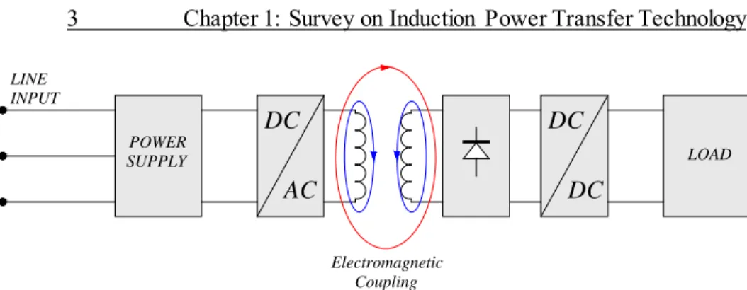
Ce dispositif présente des inductances mutuelles plus grandes que les inductances et un couplage magnétique ‘faible’ du fait de la largeur d’entrefer. La Fig. 1-2 présente l’ensemble du système de transfert par induction, pour lequel de gauche à droite nous trouvons les lignes d’alimentation par le réseau suivi d’un redresseur puis d’un convertisseur DC/AC permettant de contrôler l’amplitude et la fréquence des courants alimentant le circuit magnétique des

L’alimentation produit donc des courants sinusoïdaux de haute fréquence [10-40] kHz, les deux inducteurs constituent un système de transformateur inductif couplé dépendant de la distance de l’entrefer et nous le verrons plus tard des désalignements entre les deux (face à face non idéal). Les inducteurs ne sont pas forcément identiques et leur forme et leur composition jouent sur l’efficacité du transfert ceci sera étudié par la suite. La charge étant une charge ‘continue’ un convertisseur DC/DC sera étudié pour obtenir la régulation de tension et le contrôle des courants de la charge.

Fig. 1-2: Schéma fonctionnel d'un système IPT

L’ensemble de la conception et l’établissement du modèle électromagnétique choisi pour les inducteurs, la définition des convertisseurs et leurs circuits de compensation/résonnance, ainsi que les fonctions de transfert pour le pilotage de l’ensemble sont l’objet de cette thèse. L’objectif ici est d’obtenir un système de rechargement par induction (IPT) dynamique pour Véhicule Electrique (EV). Le design de la forme et des dimensions des inducteurs sera donc étudié en prenant en compte les contraintes d’embarquabilité dans le véhicule et de préservation de la santé humaine alentour (norme : The International Committee on Electromagnetic Safety (ICES) The International Commission on Non-ionizing Radiation Protection (ICNIRP)).

Sur la figure de principe suivante Fig. 1-3, nous pouvons considérer sous la route, une succession de circuits d’inducteurs ‘primaires’ et à bord du véhicule le système secondaire et la batterie à recharger. L’architecture sous la route peut être, soit un convertisseur multi niveau triphasé (MMC), soit une autre architecture d’électronique de puissance, l’alimentation peut se faire morceau par morceau successivement, par un simple système de détection du passage du véhicule. La difficulté ici est de gérer le fait que le véhicule passe à une certaine

LINE INPUT DC DC POWER SUPPLY DC AC LOAD Electromagnetic Coupling

hauteur (différentes gammes de véhicules) et/ou de mauvais alignement dans le plan sagittal et/ou latéral du véhicule en mouvement.

L’objectif final étant d’améliorer l’autonomie des véhicules électriques en rechargeant en cours de déplacement et donc en limitant les temps d’arrêt pour recharger la batterie.

Fig. 1-3: Architecture MMC pour l'IPT dynamique, utilisant un circuit primaire monophasé

1.2 Technologies et choix liés à l’application

En fonction de l’application visée (guidage de véhicules (AGV), chauffage par induction (heat), recharge statique (dock) ou ici recharge dynamique), le circuit magnétique peut être en I, E, H voire en S ou autres. Après une étude bibliographique et l’étude spécifique pour cette application de recharge dynamique dans un véhicule (tenant compte également de norme électrique et de sécurité de santé humaine), nous avons choisi une structure primaire et secondaire particulière et vérifié d’une part par simulation le comportement électromagnétique et d’autre part obtenu une identification des paramètres inhérents pour l’étude et le contrôle de l’ensemble.

La forme des bobines primaire et secondaire influence le coefficient de couplage magnétique d’une part, et la répartition spatiale 3D du transfert du champ magnétique d’autre part. Nous chercherons ici, un fort coefficient pour un transfert de puissance plus efficace (bon facteur de qualité à la résonnance) et une répartition ‘homogène’ du champ car le secondaire (le véhicule) se déplacera dans ce champ créé.

Nous avons donc établie les équations correspondant à ce transfert électromagnétique (Ampère, Maxwell, Faraday) reliant les facteurs de puissance et de qualité aux diverses inductances et fréquence de fonctionnement.

Nous avons également à partir de la littérature, isolé des structures de convertisseur permettant le contrôle du courant et/ou tension au primaire et secondaire du système IPT tenant compte des structures de compensation

LRp,1 LSp,1 LTp,1 LRp,2 LSp,2 LTp,2 LRp,n LSp,n LTp,n LR LS LT VR VS VT AC-GRID Ls AC DC SM_R,1 SM_S,1 SM_T,1 SM_R,2 SM_S,2 SM_T,2 SMR,n SMS,n SMT,n

développerons spécifiquement pour ce travail.

1.3 Structure magnétique

Les deux inducteurs doivent donc être relativement plats, compatibles entre eux pour un bon transfert de puissance à la même fréquence, et insensibles aux variations d’alignement voire de l’impédance de la charge tout en fonctionnant avec un entrefer relativement important (200mm).

Nous pouvons lister des circuits Circulaires Non Polarisés (trop sensible au centrage), des solénoïdes Polarisés (trop longs), des structures en Double D (DD) monté jointe ou en Quadrature (DDQ) des Bipolaires ‘entrelacés’(BP) etc. Après l’analyse des formes de la distribution spatiale de la densité de puissance et le facteur de qualité de ces PAD nous avons retenu l’association des structures DD au primaire et BP au secondaire présentant une zone d’échange trois plus grande que les autres (à dimension identique) et une moindre sensibilité aux désalignements.

La conception à partir de barres de Ferrite (type N87 forme I taille 93mm x 28mm x 16mm), des fils de Litz (section 6,36mm2_{, 810x0.1mm de résistance} négligeable) pour mieux concentrer les flux magnétiques et minimiser les pertes lors du transfert de puissance (meilleur facteur de qualité Qi), nous a permis d’obtenir une construction d’inducteur comme ci-après en restant avec des courant de l’ordre de 23A et un entrefer de l’ordre de 200mm. La structure double D polarisée Fig. 1-4 (DD Pad), combine les avantages des structures ‘circulaires’ et celles à ‘concentration’, ne présentant notamment pas de flux nul au milieu de la structure magnétique (coil1A-coil1B=L1 équivalent) et une bonne robustesse aux désalignements (faible variation d’une grande partie des paramètres caractéristiques).

Une structure carrée ‘Pad Bipolaire’ est choisie également pour mieux recevoir le transfert de puissance malgré les variations possible de positionnement du véhicule en x, y, z. Cependant ici cela implique l’utilisation de deux convertisseurs sur chacun des circuits magnétiques (Coil2-L2 et Coil3-L3) puis d’additionner les courants induits pour alimenter la charge.

Fig. 1-4: DD pad

Nous avons également établi les structures de compensation avec des capacités accordées au primaire et au secondaire (circuit LCL série au primaire et secondaire - SS compensation). Pour obtenir l’ensemble de la structure suivante présentant de bonne propriété de maintien des tensions et d’insensibilité aux paramètres de la charge ainsi qu’aux désalignements et variations d’entre fer jouant peu sur les inductances et mutuelles.

2.1 Système IPT retenu

L’alimentation principale est un redresseur suivi d’un pont en H et une capacité de sortie afin de produire des courants alternatifs carrés, cette source de courant (400 V) alimente un convertisseur résonant, le convertisseur DC/AC permet de créer le champs magnétique dans le premier circuit dans la route (5 à 50 kHz) en accord avec le circuit de compensation résonnant pour un maximum de transfert de puissance, le couplage électromagnétique permet le transfert de puissance sur les 2 parties en parallèle sous le châssis du véhicule, la puissance collectée permet la charge DC de la batterie à bord. Plutôt qu’une séparation primaire/route – secondaire/véhicule, une décomposition AC - DC s’impose.

Fig. 2-1: Diagramme de blocs, de a DD (Double D primaire PAD) BP (Bipolar secondaire) PADs

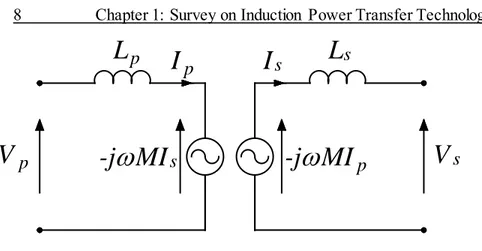
Fig. 2-2: Circuit équivalent IPT

S1 CDC + IDC Vo S2 iL4 Co + vL iL0 Rb Eb VDC d* >S2 S1 Lo L1 vref. v3 v2 L2 C2 iL2 i2 L3 C3 iL3 i3 vC2 vC3 C1 i1 iL1 iC1 i1 iC2 iC3 IDC2 IDC3 R1 R2 R3 L4 _vc0 CONTROLLER vC1

2.2 Modélisation et Analyse

A l’aide des logiciels de calcul par élément fini Flux-FEM3D, et de simulation PSIM, nous avons modélisé, calculé puis extrait les caractéristiques électromagnétiques en fonction des dimensions et formes des inducteurs et établi le circuit électrique équivalent. Nous avons également validé les performances en fonction de la fréquence d’utilisation, les désalignements en x (186, +/-140, +/-93, +/-46mm), y (+/-106, +/-80, +/-53, +/-26mm), z (150, 200, 250mm) et l’amplitude des courants.

L’analyse des différents tableaux de résultats et courbes 3D, nous montre les variations sur les valeurs des inductances propres L1, L2, L3 et mutuelles et le coefficient de couplage k.

Sur notre structure, des variations peuvent se retrouver sur les inductances propres mais pour les mutuelles des effets croisés et des symétries vont nous aider à contrôler l’ensemble.

Le calcul de la capacité de compensation C1 est fait d’une part avec les paramètres du primaire, d’autre part la capacité de compensation du secondaire C2, avec ceux du secondaire à la fréquence de 20 kHz.

La source primaire est maintenant considérée comme une source de courant alternatif (I1) de fréquence 20 kHz (AC side), le convertisseur DC/DC (DC side) fonctionnera avec un découpage de 1 kHz et un pilotage du rapport cyclique que nous développerons par la suite. Les deux bobines secondaires et leur circuit de compensation sont en parallèle pour que leur tension de sortie (Vc2=Vc3=Vdc) attaque après les deux redresseurs (non commandés ici) le convertisseur DC/DC qui alimente la charge DC (iDC).

Fig. 2-3: Comparaison entre M12 and M13

Après avoir défini les caractéristiques électromagnétiques, les dimensions et donc les valeurs des paramètres électriques équivalents, en identifiant les différentes boucles de tension et nœuds de courant, en séparant la partie AC de la partie DC, nous avons établi un modèle d’état (dimension 6 au primaire – AC et dimension 4 au secondaire – DC) afin de permettre l’étude des différentes fonctions de transfert sous Matlab entre les différentes variables courant/tension entrée/sortie etc. ' 3 2 13 1 23 2 3 3 3 3 23 23 23 ' 3 2 12 1 2 2 2 2 32 3 23 23 23 1 1 1 1 1 1 21 2 31 3 1 1

0

0

0

L DC L L L L L L DC L L L L L L L L L L

i

i

i

M i

M i

R i

L i

C

C

C

i

i

i

M i

R i

L i

M i

C

C

C

i

i

R i

L i

M i

M i

C

C



₊

₊

₊

₊

₊

₊

₌







₊

₊

₊

₊

₊

₊

₌







−

−

−

−

−

+

=





























(2.1) -200 -100 0 100 200 -200 -100 0 100 2000 0.05 0.1 0.15 0.2 x-misalignment [mm] y-misalignment [mm] M12 a nd M13 [m H]

1 1 2 2 3 3 L L L L L L i i x i i i         =                (2.2) 4 4 4 4 4 2 0 0 0 0 0 0 0 0 0 0 0 0 0 0 4 4 4 4 4 0 ˆ ˆ ˆ ₀ ˆ _{ˆ ˆ} ˆ ˆ ˆ 0 ˆ _ˆ ˆ 0 ˆ _{ˆ ˆ ˆ ˆ 0} DC DC DC DC L L L L DC C C C C DC C C L C b L C b b L C L L L L L L L dv I i C I d i D I D dt di L d V D v v d V D v D V D V V dt di L v R i V E R I dt dv C i i i D d I I I D I dt  _{+ − + + + =}    _{− ⋅ − ⋅ + − ⋅ − ⋅ − ⋅ − ⋅ + =}    _{− + − + + =}    _{+ − − ⋅ + ⋅ + − ⋅ + =}  (2.3) 4

ˆ

ˆ

ˆ

_ˆ

ˆ

dc co L Lo

v

v

x

i

i

 

 

 

=  

 

 

 

(2.4)

3

Chapitre 3 (p75-86)

3.1 Simulations de l’ensemble du système IPT

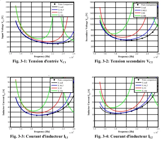
Ceci pour également vérifier la stabilité a posteriori du système et sa sensibilité aux variations d’alignements et de fréquence. Comme présenté sur les diagrammes de Bode des figures suivantes. L’étude FEM3D permet l’identification de l’ensemble des paramètres donnés à la fois à la simulation circuit (PSIM) et pour les fonctions utilisées par Matlab (respectivement points * et courbes continues). Pour le rapport cyclique fixe D=0,6, IDC entre 5 et 30A, fréquence entre 14 et 26 kHz et désalignement comme précédemment, nous

pourront être négligés.

Fig. 3-1: Tension d'entrée VC1 Fig. 3-2: Tension secondaire VC2

Fig. 3-3: Courant d'inducteur IL1 Fig. 3-4: Courant d'inducteur IL2

4

Chapitre 4 (p87-111)

4.1 Modèle et recharge contrôlée de la batterie

Après une étude bibliographique sur les différents types et caractéristiques de batterie pour les véhicules électriques ainsi que sur les types de cycles/chargeurs possibles, nous avons considérés une batterie type Li-Ion (Eb=360V, 25A) dont le cycle de recharge est conseillé en deux phases. Une phase à courant constant Io (CC) pour laquelle la tension batterie s’accroit puis une phase à tension

1.4 1.6 1.8 2 2.2 2.4 2.6 x 104 0 200 400 600 800 1000 1200 1400 1600 1800 2000 _C frequency [Hz] Input V ol ta ge VC1 [V] Psim Comparison X null X 46,5 X 93 X 186 1.4 1.6 1.8 2 2.2 2.4 2.6 x 104 0 200 400 600 800 1000 1200 1400 1600 1800 Se con dar y V ol tage VC2 [V] frequency [Hz] Psim Comparison X null X 46,5 X 93 X 186 1.4 1.6 1.8 2 2.2 2.4 2.6 x 104 0 10 20 30 40 50 60 70 80 90 100 L1 frequency [Hz] Induc to r C ur re nt IL1 [A] Psim comparison X null X 46,5 X 93 X 186 1.4 1.6 1.8 2 2.2 2.4 2.6 x 104 0 5 10 15 20 25 30 35 40 Induc to r C ur re nt IL2 [A] frequency [Hz] Psim comparison X null X 46,5 X 93 X 186

obtenir 97%).

Le convertisseur DC/DC buck/boost peut donc gérer une tension Vo plus ou moins grande par rapport à Vdc (dimensionné pour rester autour d’un rapport cyclique D de 0.5) et contrôler le courant par contrôle des switchs (S1,S2). Deux boucles de courant sont nécessaire, l’une sur Io, l’autre sur IL4.

Fig. 4-1: Buck-boost circuit et contrôle PI en cascade

4.2 Synthèse du système IPT complet

L’étude d’un simple correcteur PI est basée sur le schéma bloc suivant ayant également permis d’étudier le point de fonctionnement assurant une bonne marge de phase du système et une bande passante suffisante. Une synthèse par la méthode de Ziegler-Nichols nous a permis d’obtenir rapidement les premiers résultats en boucle fermée, deux régulateurs en cascade sont nécessaire pour maintenir les performances en courant et en tension.

Nous avons identifié certaines conditions en lien avec les possibles désalignements pour maintenir la stabilité du transfert de puissance ne remettant pas en cause les conditions de l’application visée.

S1

C

DC ₊

I

DC

V

o S2

i

L4

C

o +

v

L

i

L0

R

b

E

b

V

DC

L

o

L

4

_v

c0

i

DC d* > S2 S1 i* L4 iL4 + -i* LO iLO +

-Fig. 4-3: Schéma blocs petit signal du système DC contrôlé

4.3 Résultats du contrôle complet

Ci-après nous retrouvons l’ensemble des parties modélisées sous PSIM correspondant à l’ensemble du système IPT à contrôler pour une bonne charge de la batterie dans ce dispositif de recharge par induction dynamique.

i* L4 ₊ - Gc2(s) GdiLo(s) Gidc(s) + + io H(s) ^ H(s)i^o(s) PWM ie(s) ^ _v^_{c(s) d(s)}^ i_dc(s) ^ ac line variation ^ DC-DC Converter i ref + -^ reference input Gc1(s) GdiL4(s) i_L4(s) ^ GA(s) GB(s)

Fig. 4-4: PSIM Coupler circuit

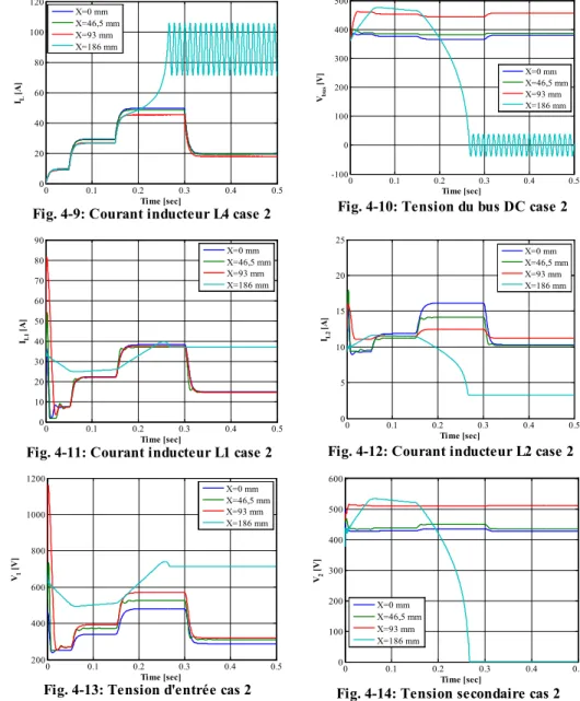
L’étude a été faite pour différents cas d’usage (valeurs différentes de Io cf cas 2 des figures ci-après), différents désalignements etc. Par exemple, pour un découpage à 1 kHz,: Vdc entre [250-400]V, Vo de 360V donnant le rapport cyclique D entre 0.41 et 0.53 nous obtenons :

Fig. 4-7: Courant de sortie cas 2 Fig. 4-8: Puissance de sortie cas 2

0 0.1 0.2 0.3 0.4 0.5 -5 0 5 10 15 20 25 30 Time [sec] Io [A] X=0 mm X=46,5 mm X=93 mm X=186 mm I_o reference 0 0.1 0.2 0.3 0.4 0.5 0 2000 4000 6000 8000 10000 Time [sec] Po [W] X=0 mm X=46,5 mm X=93 mm X=186 mm

Fig. 4-9: Courant inducteur L4 case 2 Fig. 4-10: Tension du bus DC case 2

Fig. 4-11: Courant inducteur L1 case 2 Fig. 4-12: Courant inducteur L2 case 2

Fig. 4-13: Tension d'entrée cas 2 _{Fig. 4-14: Tension secondaire cas 2}

0 0.1 0.2 0.3 0.4 0.5 0 20 40 60 80 100 Time [sec] IL [A] X=46,5 mm X=93 mm X=186 mm 0 0.1 0.2 0.3 0.4 0.5 -100 0 100 200 300 400 Time [sec] Vbus [V] X=0 mmX=46,5 mm X=93 mm X=186 mm 0 0.1 0.2 0.3 0.4 0.5 0 10 20 30 40 50 60 70 80 90 Time [sec] IL1 [A] X=0 mm X=46,5 mm X=93 mm X=186 mm 0 0.1 0.2 0.3 0.4 0.5 0 5 10 15 20 25 Time [sec] IL2 [A] X=0 mm X=46,5 mm X=93 mm X=186 mm 0 0.1 0.2 0.3 0.4 0.5 200 400 600 800 1000 1200 Time [sec] V1 [V] X=0 mm X=46,5 mm X=93 mm X=186 mm 0 0.1 0.2 0.3 0.4 0.5 0 100 200 300 400 500 600 Time [sec] V2 [V] X=0 mm X=46,5 mm X=93 mm X=186 mm

Fig. 4-15: Courant de sortie avec un désalignement x=186 mm

Un courant Iref de plus de 14 A rend instable le contrôle, cela correspond à une limitation à un maximum de 5 kW. Cependant le comportement est efficace et correct même pour des désalignements en x de 93mm (moitié du dimensionnement choisi, 193 mm rend également instable mais ceci est ‘normal’ du fait que le véhicule n’est plus du tout au-dessus de l’inducteur primaire). L’étude est également faite sur les désalignements selon l’axe y.

5

Chapitre 5 (p112-113)

Conclusions générales : La thèse a montré la faisabilité d’un système de recharge par induction pour la recharge de la batterie d’un véhicule électrique en mouvement. Pour cela une étude bibliographique a permis d’isoler le dispositif adapté pour un bon transfert de puissance. Le design des inducteurs et l’extraction des paramètres ont permis de caractériser le comportement électrique de l’ensemble. L’exploitation des expressions mathématiques des parties alternatives, continues, et le coupleur ont permis l’analyse des Bodes en fonction des désalignements possibles. Une simulation complète PSIM, complétée par la synthèse d’un contrôleur du convertisseur de charge de la batterie montre les conditions de fonctionnement dans certaines limites principalement liées aux dimensions imposées par les dimensions du châssis et donc les désalignements à respecter.

0 0.1 0.2 0.3 0.4 0.5 0 2 4 6 8 10 12 Time [sec] Io [A] I_reference=5 A I_reference=10 A I_reference=14 A I_reference=15 A

1.

Chapter 1

Survey of Induction Power Transfer

1.1 Introduction

1.1.1 Overview of Inductive Power Transfer System

Inductive Power Transfer IPT is the most widespread methods of wireless power transfer. IPT is applicable to many power levels and gap distances. Almost all wireless power transfer techniques use near field electromagnetics induction. Ampere’s circuital law and Faraday’s law of induction are the two principles on which is based the IPT systems. Ampere’s law states that a magnetic field is produced around a conductor carrying electric current with a strength proportional to the current, whereas the Faraday’s law states that an alternating magnetic field can induce an electromotive force in a conductor that is proportional to the magnetic field’s strength and its rate of change. The first use of wireless power transfer has been possible thanks to Nikola Tesla around 1891. He invented the Tesla Coil, an electrical resonant transformer circuit, used to conduct innovative experiments among which the transmission of electrical energy without wires. Although the principle of function is at the base of modern solution, the diffusion of IPT system has been possible only at the end of 20th _{century because of component limitations at the time.}

Fig. 1-1 illustrates how work an elementary IPT system. In the simplest form, an IPT system consists of two physically detached coils. When an alternated current flow in the first coil, called transmitter coil, a magnetic field is produced.

If the second coil, called receiver coil, is placed in close proximity with the transmitter, the alternating magnetic field will induce an electromotive force in the receiver’s coil. A current will flow in the load if it is connected to the receiver coil. In these circumstances the power is transferred by induction from one coil to another without physical contact much like in a transformer but,

unlike this latter, it has a low value of magnetic coupling. These system, in fact, have a leakage inductance higher than they magnetic inductance and therefore they are called loosely coupled system. Such power transfer is clean, unaffected by chemicals or dirt.

Fig. 1-1: Elementary IPT system

The Fig. 1-2 shows the block diagram of a typical IPT system. It can be noted that the system is splitted into two electric subsystems, magnetically coupled and supplied by means of high frequency power converter.

An IPT system comprises three main components: a power supply, almost two coupled coils, a rectifier and DC/DC converter. The power supply produce a sinusoidal current, with a usually frequency of 10-40 kHz, that flows in the transmitter coil. The power flows to the second subsystem by means of inductive link constituted by the two coupled coils. The two coils are not necessarily identical, they could have different dimensions and shapes. The rectifier may be required to transform the high frequency ac voltage into dc voltage if the load to be powered is a dc load. Moreover, an additional DC/DC converter can be required to provide a regulated input dc voltage to the load.

Fig. 1-2: Block diagram of a typical IPT system

1.1.2 Aims and Objectives of thesis

The aim of this thesis is design an IPT system, applied to the refill of batteries on board of the Electric Vehicles EV. The work has been done following the below objectives:

• Overview of the current state of EV’s IPT technologies; • Choose of a proper topology of system;

• Design of magnetic structure; • Modelling of the system; • Control of the system;

1.2 Induction Power Transfer Technology

1.2.1 Introduction

Due to oil rarefaction and gas emission restrictions, there is a growing interest all over the world for introducing electrical propulsion for ground transportation. Hybrid electrical vehicles are a first step for this energy transition, changing oil consumption in internal combustion engine to clean electric consumption in full electric vehicle. Nowadays hybrid and full electric vehicles suffer for some main drawback: their autonomy, the high initial cost (essentially battery costs), an excessive charging time not comparable to that of conventional vehicles and absence of a wide network of charging station. This project takes advantage of future trends on road architecture evolution including in the road possible induction and charging stations (ever existing in metro and tram systems). The vehicle autonomy can be extended reloading the battery during the trip. This

LINE INPUT DC DC POWER SUPPLY DC AC LOAD Electromagnetic Coupling

concept has been referred to as dynamic charging, move and charge or roadway powered EVs. Dynamic charge can mitigate the high initial cost of plug in EVs by allowing to undersize the battery on board vehicle and could reduce the cost, the weight and fuel consumption of the vehicle. In addition, dynamic charging can provide a very effective utilization of the installed infrastructure, since a large number of vehicles use the same road segments that can be dynamic charge enabled. This is challenging and a complete design and model of the induction system should be established and local and global control made.

In this thesis, a complete study is presented from the road and truck inductors design. Parameter identification is achieved using electromagnetic flux software, thus equivalent electric circuit is deduced and also parameters variations are studied due to possible misalignment in case of such mobile devices more particular than reloading systems at fixed dock. At last, a state-space formulation is obtained representing the current, voltage and Induction Power Transfer behavior for analysis and control purposes.

1.2.2 Current Application and Technologies

The IPT technology is not based on recent concepts. The first person that has introduced the concept of wireless power transfer was Nikola Tesla around 1891 beginning from the Ampere and Faraday laws. He invented his famous Tesla coil. The system contains two loosely coupled and tuned resonant circuits: a primary and a secondary. Periodic spark gap discharges were used to short out the primary resonant circuit and initiate the power transfer. Tesla’s experiments demonstrate the majority of modern IPT design concept: a resonant circuit has needed to enhance the power transfer; a resonant converter has needed to supply the primary coil. The IPT was considered to be not viable for some time and against a background of unbelief it was not until the end of twentieth century that real commercial IPT system appeared.

An IPT system involves the coupling of two or more coils. When an alternated current flow in the first coil if the other coils are placed in close proximity with the first, the alternating magnetic field will induce an electromotive force in each coil. Such power transfer is without physical contact, clean, unaffected by chemicals or dirty and has the capacity to revolutionize many manufacturing processes. IPT finds application in factory automation, for instrumentation and electronic systems, in biomedical implants, in security systems, harsh environments and a lot of other applications where its unique features can be exploited. In fact, early commercial IPT systems found

applications in car assembly plants where tolerance to paint and welding fumes was highly prized and also in transcutaneous medical devices while the dynamic powering of vehicles on monorails has spread to floor mounted automatic guided vehicles (AGV). Although the developments in this technology began with industrial applications, recently have shifted to designs that can meet the challenge of powering electric vehicles under both stationary and dynamic conditions.

In all such IPT systems thus far, energy has been coupled from a primary to a secondary across an air gap of significant but small proportions that stays relatively constant, even in the presence of movement. In manufacturing application, one primary circuit was able to drive a multitude of secondary circuits. Track guidance systems allow vehicles without drivers to move along a current carrying conductor. The inductive method has the advantage that it is not sensitive to oil, dirty, tire abrasion etc. Thus, their use has gained acceptance in harbors and industrial plants. Reference frequency and current as well as lateral separation and height from guide conductor can be selected from a large scope of variants. This type of systems are called automated guide vehicle. An AGV is a driverless transport system used for horizontal movement of material. They are most often used in industrial application to move materials around a manufacturing facility or warehouse. AGVs are employed in nearly every industry, including, pulp, paper, metals, newspaper and general manufacturing. The first AGV was brought to market in the 1950s and it was simply a tow truck that followed a wire in floor instead of a rail. The use of AGVs has grown enormously since their introduction. The primary coil on a monorail has the form of an elongated loop that is loosely coupled to a pickup coil on a vehicle and may transfer 1-10 kW of power across a 4-10 mm gap. With an AGV, the air gap may be 10-20 mm, and there may be a possible misalignment of similar magnitude.

An IPT system for the charging of the vehicles may be considered as an evolution of IPT system used in industrial application for the movement of products within an establishment. Differently of the AVG systems, for the EV charging of IPT systems, the trend is to use two concentrated coils, called pad, one buried in the roadway and the other mounted on the chassis of the vehicle.

1.2.3 Fundamental Principles of the IPTS

Modeling the IPT system is crucial in designing wireless power transfer system for EVs. Simplicity and the accuracy of the model are important. The modeling

methodology needs to provide guide lines in the selection of system performance indices and design parameters.

A power supply takes power from a utility and energizes a primary loop or track to which pickup coils may be magnetically attached. In Fig. 1-3, is shown a typical scheme.

Fig. 1-3: Block diagram of a typical IPT system

In the simplest case, an IPT pickup consists of a coil of wire in close proximity to the track wires positioned to capture magnetic flux around the track conductor. Conceptually, this is similar to a transformer, although with a much lower magnetic coupling. As in transformer design, magnetic material such as ferrite is used to direct the magnetic flux and improve the coupling between the track and any pickups.

The IPTs are governed by Ampere’s law and Faraday’s law among four Maxwell equations, as shown in Fig. 1-4.

It can briefly explain as follows:

1) time varying magnetic flux is generated from the ac current of a power supply rail in accordance with Ampere’s law;

2) voltage is induced from the pickup coil, coupled with the power supply rail, in accordance with Faraday’s law;

3) power is wirelessly delivered through magnetic coupling, where capacitor banks are used to nullify inductive reactance.

The governing equations of IPTS for sinusoidal magnetic field, voltage and current are approximated as follows:

∇× =

H J

_(1.1)

jω

∇ × = −E _{B (1.2)}

Fig. 1-4: Maxwell equations

In the development of a complex technology such as this it became impossible design and work with a circuit constructed of wire, ferrite, air gaps and electronics components so an electrical equivalent circuit had to invented as shown in Fig. 1-5. B E t ∂ ∇ × = − ∂ C S d E dl B dA dt ⋅ = − ⋅

∫

∫

�

D H J t ∂ ∇ × = + ∂ C S S d H dl J dA D dA dt ⋅ = ⋅ + ⋅

∫

∫

∫

�

1

E

=

j MI

ω

N1I1 A m p e re ’s L a w Far aday ’s L aw

Fig. 1-5:Equivalent coupling circuit

The performance of an IPT pickup is primarily determined from two parameters 0: the open voltage circuit voltage induced in the pickup coil at frequency ω due to primary track current I1,

V

_oc

=

j M I

ω

1and its short circuit current

I

sc

=

M I L

_{1 2} which is the maximum current from

V

oc limited by the

impedance of the pickup coil inductance

ω

L

₂. Here, M is the mutual inductance between the track and the pickup coil. From the first principles, the product of these two parameters is the maximum VA rating for the pickup called Su and give a measure of how good the power coupling of any magnetic system is for a particular driving condition.

2 2 1 2 u oc sc

M

S

V I

I

L

ω

=

=

(1.3)

without compensation, the maximum power that can be drawn from a pickup is generally not sufficient. In order to improve the available power, the pickup inductor is compensated with capacitors such that it resonates at or near the frequency of the track.

The ac tuning causes a resonant current to flow in the tuned

L C

_{2 2} circuit, which is boosted by Q2, while the voltage

V

c across the capacitor is similarly

boosted by the circuit Q2. Here, Q2 is the tuned quality factor of a secondary system, which is determinate by the output load or controlled by controlling the output voltage current.

L

s

I

s

V

_p

-j

ω

MI

_p

V

s

L

_p

-j

ω

MI

s

I

_p

Thus, for the parallel tuned regulator, this tuning enables the output voltage seen by the regulator to be increased in proportion to the circuit’s resonant Q, while for a series tuned pickup, the output current is boosted by Q. In either case, the maximum power that the system can transfer into a load is thereby improved by Q2resulting in 2 2 2 1 2 2 out u

M

P

S Q

I

Q

L

ω

=

=

(1.4)

This power equation is valid for all manner of IPT systems but some minor adjustments may occur in track based systems driven from a current source when the inductance L1 can be very large. Pickups in track systems are usually in a close relationship with the track and can partially enclose the track inductor giving high k values (where

k

=

M

L L

1 2 is the magnetic coupling factor) that are not achievable with floor mounted system such as AGVs or moving robots. Nonetheless, regardless of the value of k the analysis can proceed in the same way. The magnetic coupling coefficient is a very important parameter determining the performance of IPT system. In fact, the output power of an IPT system can be easily quantified as a function of the magnetic coupling coefficient k by means of the following relation:

2 2 2 2 1 2 1 1 1 2 1 1 2 2 1 2 out

M

M

P

I

Q

L I I

Q

V I k

Q

L

L L

ω

ω

=

=

⋅

=

⋅ ⋅

(1.5)

In this form, the power transfer can be seen as the input VA multiplied by the magnetic coupling factor k2_{, multiplied by the electrical quality factor of the} loaded secondary circuit Q2 and is not dependent on ω that is now included in the voltage at the input of L1.

Following (1.5), the power transferred by an IPT system can be improved by increasing any of ω, M, I1 or Q2. There are, however, advantages and disadvantages with all of these possibilities. Increasing the power by increasing the frequency is something of an illusion and may not bring about the benefits expected. The system is clearly frequency sensitive but it is not a simple dependency as it appears here. Increasing the mutual coupling is without doubt the best solution as it involves making the magnetics better and as this is a magnetic coupling it is really the ideal approach, but there are limits in terms of magnetic coupler size and volume of material that must be considered for each application. Increasing the excitation current is a forced solution that usually

leads to a lower efficiency. It will give more power, but it puts more stress on all the components in the process. Increasing Q2 of the secondary electrical circuit is a good solution but as described below this increases the VA of the secondary and narrows its bandwidth (much in the same sense as tuning a radio receiver). It cannot be carried to excess or the system becomes too difficult to tune and keep on tune over time (because of aging effects of capacitors) or in uncontrolled environments (where the presence of materials or movement can shift the inductance value).

1.2.4 Components of an IPT System

A simple IPT system is shown in Fig. 1-3. It comprises of the following:

1) a power supply that takes electric power from a utility or a battery; 2) an elongate track that is driven by the power supply whereby current

in the track causes a magnetic field that follows the track;

3) pickups on or along the track that intercept some of the magnetic field and convert that intercepted field to controlled electricity; 4) electrical loads that may be driven by that electricity.

All of these aspects are important but some are essentially self-evident. There are a very large number of power supply circuits that may be used in an IPT system but all of them achieve the same outputs with different output frequency, efficiency, and reliability. However, modern IPT supplies generally

favor current controlled supplies with unity power factor and with a controlled frequency [2]. The frequency must be system wide but other attributes will vary with cost and availability. The track usually uses high frequency Litz wire to support the magnetic field.

A significant effort in the design of IPT systems is to increase k by improving the magnetic designs.

1.2.5 IPT Power Supply

A DC-AC inverter is a common solution to generate a high frequency track current for an IPT system. Often a front-end low frequency mains power is rectified into a DC power source and then inverted to the required high frequency AC track current. Energy storage element, such as large DC capacitor, are used to link the rectifier and the inverter. IPT power supplies may be voltage sourced or current sourced, and may be a full bridge or half bridge

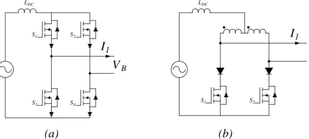
configuration. Fig. 1-6 shows circuits for voltage sourced inverters for both full bridge or half bridge and Fig. 1-7 shows circuit for current sourced inverters again for both full bridge and half bridge.It should be noted that no one circuit is fundamentally better or worse than any other circuit and there is a lot of designer choice but that said some of the circuits do have some features that are particularly attractive.

Fig. 1-6: Voltage source inverters: (a) full bridge, (b) half bridge

Fig. 1-7: Current source inverters: (a) full bridge, (b) half bridge

When used in an IPT system the track requires a constant current along its full length so that pickups at any point along the track operate under their design conditions. In principle, this may be achieved using one of the circuits in Fig.

S4

(b)

I

₁ S1 LDC

V

_B S2

(a)

S2 S1 LDC S3

I

₁

I

₁ S3 S4

(b)

I

1

V

_B S1 LDC S2 S1

(a)

LDC S2

1-8 where Fig. 1-8 (a) is parallel tuned and can operate with an inverter supplying an output voltage and virtually no other control, while Fig. 1-8 (b) is series tuned and the inverter itself must supply all of the output current and will need some form of controller.

At this point there is a major difference between these alternatives: for a track current of 100 A say the inverter of Fig. 1-8 (a) only has to supply the real load current which is typically a lot less than the 100 A while the inverter of Fig. 1-8 (b) must supply the whole of the 100 A meaning that there is always 100 A in the switches of the inverter and this circuit is therefore likely to be less efficient especially on lighter loads. Today there is another option – shown in Fig. 1-8 (c).

Fig. 1-8: Fixed frequency supplies: (a) parallel tuned; (b) series tuned; (c) LCL compensation using extra inductor

Here an impedance converting network (an ICN) called here an LCL-T circuit is placed between the inverter and the parallel tuned load of Fig. 1-8 (a) to give a constant current in the track provided that the inverter outputs a constant voltage. So Fig. 1-8 (a) and Fig. 1-8 (c) give the same current in the track but the difference is that the power factor of the inverter current in Fig. 1-8 (a) may be poor so that the inverter will have to work harder whereas the power factor with Fig. 1-8 (c) is perfect and the inverter sees a resistive load with perfect tuning.

Modern industrial IPT power supplies have a level of performance that would have seemed impossible 3-5 years ago. Today power supplies are modular so that the economy of scale can be brought to larger units. An attractive solution is to supply the IPT system by means of a Modular Multilevel Converter MMC. Its basic architecture is shown in Fig. 1-9.

INVERTER C1 L2 Ltrack Itrack Ltrack C1 (a) Ltrack INVERTER C1 (b) Itrack INVERTER Itrack (c)

Fig. 1-9: a) Modular Multilevel Converter architecture; b) structure of a sub-module Usually, each converter leg includes freely chosen number n of identical sub-modules. The main advantages, that make very attractive this circuit topology, are: a modular structure able to be adapted to different voltage and power levels; a redundant operation that performs high availability values and robust failure management (i.e. a sub-module can be short-circuited, while the corresponding leg can still operate with one voltage level less, but without any further restriction).

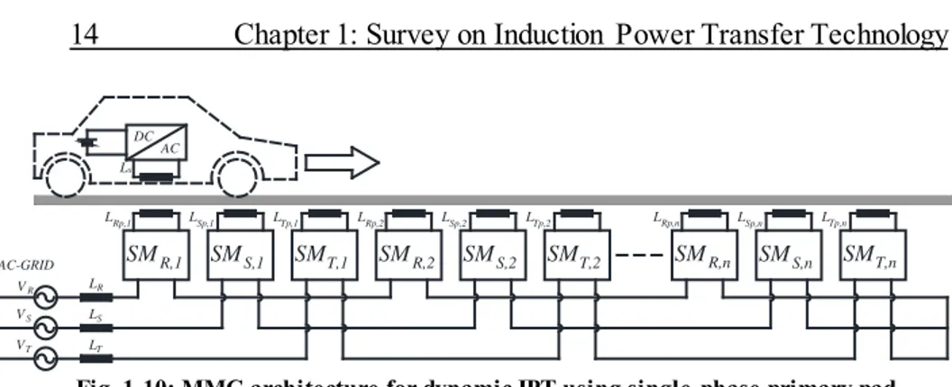
Obviously, the converter architecture should be adopted to the used primary pad. Using this topology of converter to dynamic charge, when the primary pad is single-phase, the architecture is shown in Fig. 1-10. Once, the path is defined and also its length is established, then the primary pads are buried sequentially along the path by leaving a proper gap among them. Each primary coil pad is fed by a single sub-module of the. Moreover, the pads order must be as reported in Fig. 1-10 (e.g. LRp,i, LSp,i, LTp,i, with i=1,…,n). by detecting the vehicle position versus path [3], only the pads covered by the vehicle are energized. The total number of primary pads must be multiple of three, in order to have the same number of sub-module for each leg phase.

AC - Grid iT ……. La iR iS EB,1 Side (a) LRp,1 Ac/Dc Ls,1 SMn SM2 SM1 LSp,1 LSp,1 LTp,1 LRp,2 Ac/Dc Ls,2 EB,2 Side LRp,n LSp,n LTp,n Ac/Dc EB,n Side ……. AC Side SideEB H bridge H bridge HFPrimary

Magnetic Pads Storage + Buffer SMi i=1,..,n (a) Battery (c) (b) Secondary H bridge HF

Fig. 1-10: MMC architecture for dynamic IPT using single-phase primary pad Furthermore, if the primary pad is a tripolar pad, the converter architecture is shown in Fig. 1-11. The tripolar pads are buried sequentially along the path by leaving a proper gap among them. Each pad consists of three coils fed by three subsequent sub-modules of the same phase leg. Thus, the series of three primary tripolar pads are fed by three different phases. The total number of primary pads must be multiple of three, in order to evenly the load of each phase.

Fig. 1-11: MMC architecture for dynamic IPT using three-phase primary pad L_Rp,1 L_Sp,1 L_Tp,1 L_Rp,2 L_Sp,2 L_Tp,2 L_Rp,n L_Sp,n L_Tp,n LR LS LT VR VS VT AC-GRID Ls AC DC SMR,1 SMS,1 SMT,1 SMR,2 SMS,2 SMT,2 SMR,n SMS,n SMT,n LRp,1 SM_R,1 LRp,2 LRp,3 LR LS LT VR VS VT AC-GRID Ls AC DC SM_R,2 SM_R,3 LSp,1 LSp,2 LSp,3 LTp,1 LTp,2 LTp,3 LTp,n-2 SMT,n-2 LTp,n-1 LTp,n SM_S,1 SM_S,2 SM_S,3 SM_T,1 SM_T,2 SM_T,3 SMT,n-1 SMT,n

1.2.6 Pickup Regulator

Fig. 1-12:Pickup equivalent circuit

In order to refill the battery mounted on board of the electric vehicle, it is necessary convert the alternating AC current to the direct DC current by means of a rectifier converter [4]. The output voltage of the secondary pad depends from several factors, among which the coupling factor has a strong impact. Obtain a proper value of the output voltage may be difficult in consideration of the different airgap, misalignments, so it is indispensable have a system of the control. A possible solution to control the power flow, can be achieved using the switch mode controller by using an DC/DC converter. The output charge current of the pick-up may be determine operating on the DC/DC converter. A possible DC/DC converter, in particular a buck boost converter, is propose in the following Fig. 1-13:

Fig. 1-13: Buck boost converter

Using this converter, the voltage output or the current output may be kept equal to the reference value, independently to the value’s voltage input.

M

C

DC S LOAD

L

DC

V

o

i

₁

C

₂

L

₂

V

OC

S

1

L

L

o

C

o

R

b

C

DC

I

DC

S

2 +

V

o

Io

v

c0 +

v

L

i

L

V

DC

E

b

1.2.7 Control Strategies

The power supply and primary controller normally control both the frequency and the primary current to achieve maximum power transfer capability. Both fixed and variable frequency controllers can be used. Power flow regulation is also required because of variations in load and other system parameters.

1) Power flow regulation: one common approach to achieve power flow regulation is detune the system by shifting the operational frequency of the power supply. This approach is not suitable for many multiple pickup applications where the load condition on each pickup can be different. Here, detuning the power supply affects all the secondary pickups so that some pickups may be unable to deliver the necessary power. An alternative approach is to use a switched mode controller within the secondary pickup for power flow control. Using this approach, each pickup can be controlled separately or even decoupled completely from the primary. However, the disadvantages are increased switching losses and a higher cost of the secondary pickups.

2) Fixed frequency control: with fixed frequency, controlled applications, variations in load and coupling between the primary and secondary will cause a phase shift in the load impedance. If this phase shift is significant, then the power supply must have a higher VA rating for the same power transfer.

3) Variable frequency control: most variable frequency controllers operate at the primary ringing frequency. However, the operational frequency will shift away from the load and the degree of coupling between the primary and secondary. This results in a loss of power transfer capability if the frequency shift is too large and may also result in a loss of frequency stability and controllability because of the onset of bifurcation with increasing load, where more than one primary was phase angle frequency exists.

1.2.8 Magnetic Structures

IPT systems use two or more magnetic couplers to transfer power from one frame of reference to another. The most important factor in an IPT system is the magnetic coupling coefficient k and techniques that increase k lead directly to systems that can transfer power more efficiently than others.

In function of type of application, the magnetic structure may be different. In factory automation FA, IPT systems are chosen for their tolerance of dirt in welding bays and paint shops; in Clean Factory Automation (CFA) situations,

IPT systems are chosen for their cleanliness and residue free applications. Pickups in these and other factory applications were widely named according to the letter of the Latin alphabet that they most closely resembled for example I, E, and H but other shapes were also suggested, for example an asymmetrical S pickup is difficult to mount but gives almost twice the available power as a symmetrical E pickup for the same material cost [5]. A feature of all of these pickups was that they operated with relatively small air-gaps, and good coupling factors at high efficiency. As the technology and its applications developed these ideal operating conditions, however, became more stressed. Floor mounted systems, generally use two wires 100 mm apart buried under 10 mm of concrete, each with a current of 125 A at 20 kHz. In their primitive form, they used a flat E pickup to achieve coupling factors within 50% of those attainable with a monorail. In monorail applications, the tines on the E and H pickups could encircle the track to 270° whereas floor mounted pickups could not encircle even to 180° giving a low output but they could sense the wire position under the concrete floor and use this information to navigate around the factory. Also, in a new innovation, extra coils could be added to the flat E ferrite converting it into a quadrature pick up where both the power profile and the tolerance to misalignment are enormously improved [reference]. The floor mounted pickups do, however, have the whole track energized all the time and as this may be as long as 300 m it does create a large area in the factory closed to personnel.

Overhead monorails have a track 3,4 m high and this makes them inherently safe but not usable for EVs.

In construction, couplers are fragile and means must be found to protect the coils from damage. The protection usually entails packaging the coils in soft plastics or rubber materials that add significantly to the bulk of the pickup without adding to its function. IPT systems for charging EV batteries, can be seen as an extension of the technology for industrial floor mounted systems and are gaining attention for their convenience of use.

The systems are however quite different as they do not use a track (elongate) but use two wireless pads one on the underside of the vehicle and the other on or under the road surface immediately under the vehicle. With FA system, the misalignments and their air-gaps are small but in the EV application they can be large.

The biggest difficulty of all is that unlike FA, people are, however, commonly near to EV charging equipment and the emission from the vehicle must be contained below international standards [6], [7]. The pads are magnetically coupled to each other.

Fig. 1-14: Factory automation IPT system: the core are called U, E, S, H, I and Flat E corresponding to (a), (b), (c), (d), (e), (f) respectively.

This wireless power transfer uses inductive coupling under resonance with coils or multiples of coils with high native quality factor (QL). The coupling is a geometrical property of the magnetic and electrical circuits: better pads achieve coupling depending on their design and a poor design can never be adequately compensated but leads inexorably to a poor IPT system. Early commercial designs were developed in the 90’s and have been improved over the past 20 years. As noted before this inductive coupling is a strongly coupled magnetic resonance.

For efficient charging with minimal field leakage the car must be parked or positioned so that the two pads are in relatively close proximity to each other. Under these conditions a recognition system allows the two pads to communicate with each other such that ultimately the pad on the ground is fired up and energy is transferred from the ground pad to the on-vehicle pad and thence to the battery. When the battery is charged, the system disconnects and both the ground pad and the vehicle pad are shut down.

Wireless EV charging via IPT can only occur if several conditions are met simultaneously:

- The pads must be compatible with each other;

- The position of the car must have the on-vehicle pad within the relative x, y, z, error that is allowable for this pad pair;

- The communications protocol must be compatible between the two pads;

- The power ratings and connections of the two pads must be designed to be compatible and at similar rating.

Traditional, practical couplers for EV systems are either circular in shape with a coil in the form of a flat Archimedean spiral placed in magnetic material or shaped like a solenoid using a cylindrical spiral with a magnetic material through the middle of the coil. Such systems have evolved from essentially track based designs to concentrated couplers. In the early system, the essential problem that limited was the unavailability of modern materials. Without ferrite and Litz wire, the pickups are too heavy and without modern power electronics the frequency are too low rather than 20 kHz or higher. In consequence, while the concepts and designs were well thought out, the tolerance for parking or moving is highly constrained, and the cost was too high.

Power pads need to fulfil several requirements to enable practical application on an EV. The pads should be as thin as possible for ground clearance and fitting, operate with a large air gap, be lightweight to minimize vehicle energy requirements and have good tolerance to misalignments to allow easier parking. Designs using pot cores [reference], U cores or E cores are unsuitable for EVs due to excessive thickness or fragility since large pieces of ferrite are required. These topologies are also necessarily sensitive to horizontal misalignment because the coupling surfaces are relative small compared to the size of the pad. The lumped magnetic pad designs used in single point charging applications are generally categorized based on their ability to generate or couple only the parallel, perpendicular or both components of flux entering or leaving the pad surface. A non-polarized pad design ideally generates and couples a flux pattern that is symmetric around the center of the pad, but the term is still used for the pad designs where the fields are directionally symmetric around the pad center though the strength of the field might be different along different angles around the center. On the other hand, a polarized pad generates and couples a flux pattern in which the flux flows dominantly along one dimension of the pad only, in example, either length or width of the pad.

1.2.9 Circular Non-Polarized Pads

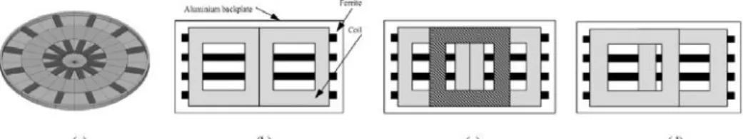
For medium and high power, single point charging application using lumped primary and secondary pad designs, the proposed system that utilizes the non-polarized perpendicular flux generation approach consists of an identical circular pad primary and secondary. This pads, derived from pot cores, are designed to generate a single sided flux pattern [8]. Therefore, these pad designs have a coil structure followed by a ferrite structure and an aluminum back plate structure on one side to facilitate a low reluctance flux path while reducing the leakage flux in the back of the pad, with the other side facing on the second pad in the system. As shown in Fig. 1-15, the circular pad consists of a single coil and generates a flux that is symmetric around its center, which also explains a ferrite structure symmetric around the center of the pad.

Fig. 1-15: Circular pad

This circular coil adopts ferrite bars instead of ferrite plates to have a compact structure, low weight and low EMF. These are important characteristics because at present EV and PHEV manufacturers are interested in smaller vehicles with low ground clearances giving air-gaps between the primary and secondary pads. In Fig. 1-16, has shown a view of a circular type coil proposed by a team research of Auckland University. It has six main components. The aluminum ring and backing plate add robustness and provide shielding around the pad to leakage flux.

Fig. 1-16: Circular type coil using ferrite bars

In [8], [9], has shown that the ideal coil diameter of a circular pad is 57% of the pad diameter that includes an aluminum ring. The relationship between the size of a pad and its ability to throw flux to a secondary pad placed above it has been explained using the concept of fundamental flux path height [10]. As reported in [8] the fundamental flux path height (Pd) is proportional to half of the ferrite length which is only one quarter of the pad diameter (Pd/4). Therefore, such pads are suitable for stationary charge system and have values of k about 0,17 at height almost four times lower than the pad diameter. This means it is necessary to use pads with excessive diameter.

Unlimited EV range can be realized with dynamic charging system however the receiver on the EV must work equally well with both stationary and moving transmitter pads. Circular pads are not suitable for dynamic charging as they have a null in their power profiles when horizontally offset by 38% of the pad diameter [8]. The null occurs within the pad diameter so even if transmitter pads are touching along the highway, it is not possible to obtain a smooth power profile.

1.2.10 Solenoid Polarized Pads

In order to obtain a desirable coupling coefficient whit air gaps in the range of 150-250 mm, the diameter of a circular pad needs to be increased significantly