3621 Page 1
Performance analysis of a mini exhaust air heat pump integrated into a low
energy detached house: experimental on-site performance
Frédéric RANSY
1*, Kevin SARTOR
1, Samuel GENDEBIEN
1, Vincent LEMORT
1 1University of Liege, Thermodynamics Laboratory,
Liege, Belgium
* frederic.ransy@uliege.be
ABSTRACT
This paper presents the on-site performance of a mini exhaust air heat pump integrated into a low energy detached house situated in Belgium. The system consists of five components: a simple exhaust ventilation system, an exhaust air heat pump, a backup electrical resistance for space heating only, a domestic hot water storage tank and fan-coil units to heat the building. In that system, the heat source of the heat pump is the air from the ventilation system and the heat pump heating capacity is limited to 1500 W. During the night, the exhaust air heat pump produces the sanitary hot water, which is stored in a water tank. Consequently, the totality of the domestic hot water is produced by the heat pump. During the day, the heat pump can also be used to heat the building. Nevertheless, only a part of the energy requirements related to heating are covered by the machine, due to the limited heating capacity. The remaining heating requirements are covered by the backup electrical resistance. For this reason, this machine is particularly suitable for apartment buildings characterized by a low heating demand and a significant energy demand related to domestic hot water production. In the first part of the paper, the characteristics of the building case study and the different components of the system are presented. The second part of the paper describes the sensors placed in the building used to measure the on-site performance of the machine. In the third part of the paper, the on-site performance of the machine is presented. The influence of the main variables (exhaust water temperature, supply air temperature, outside temperature) on the performance is also discussed. In the last part of the paper, the performance of the whole system is estimated for a typical meteorological year. The estimation is based on the Energetic Performance of Building certificate of the building, and on empirical relationships established with the on-site performance of the machine.
1. INTRODUCTION
Buildings are responsible for 40% of energy consumption and 36% of CO2 emissions in the EU (European Commission, 2010). In order to reduce this energy consumption, the European Commission proposed two Directives: the Energy Performance of Buildings Directive (European Commission, 2010) in 2010 and the Energy Efficiency Directive (European Commission, 2012) in 2012. In that context, Member States need to make significant efforts to improve the energy efficiency of buildings.
Two key measures are generally implemented: an increase of the thermal insulation and the improvement of the airtightness. As a result, a mechanical ventilation is required to ensure a good indoor air quality and the ventilation has a more significant impact on the building energy consumption, accounting for 30 to 60% of the total building energy use (Orme, 2001). For these reasons, a mechanical ventilation system with a highly efficient heat recovery is installed in the majority of new and retrofitted residential buildings.
In Belgium, in new residential buildings, a typical HVAC systems configuration consists of a balanced ventilation system with heat recovery combined with an outside air heat pump used to heat the building and produce the domestic hot water. According to the UCL energy institute (2017), the seasonal COP of this type of heat pump varies from 2 to 3, with an average value of 2.44.
Theoretically, a higher seasonal COP could be achieved by using an exhaust air heat pump combined with a simple exhaust ventilation system. In that system, the heat source of the heat pump is the exhaust air from the ventilation system. The temperature of the exhaust air is rather constant during all the year and is typically equals to 20°C. Moreover, if the heat pump is sized appropriately, the energy losses due to frost formation on the evaporator can be prevented. For these reasons, the seasonal COP can theoretically be comprised between 3 and 4 (Fracastoro and
3621 Page 2
Serrain, 2010). However, the ventilation losses of a simple exhaust ventilation system are higher, and an analysis on the whole building must be conducted in order to correctly estimate the performance of the system.This paper presents the on-site performance of a mini exhaust air heat pump that is combined with a simple exhaust ventilation system. In that system, the heat pump heating capacity is limited to 1500 W and the totality of the domestic hot water is produced by the heat pump.
2. DESCRIPTION OF THE SYSTEM
2.1 Building characteristics
Geometry. The building case study consists of a new residential building built in 2016. It is a wooden two-story
freestanding house whose geometry is typical of new residential buildings in Belgium. An unoccupied attic is also included into the heated volume. The total floor area is 155 m², the total heated volume is 583 m³ and the total exposed area is 389 m². The
𝑛
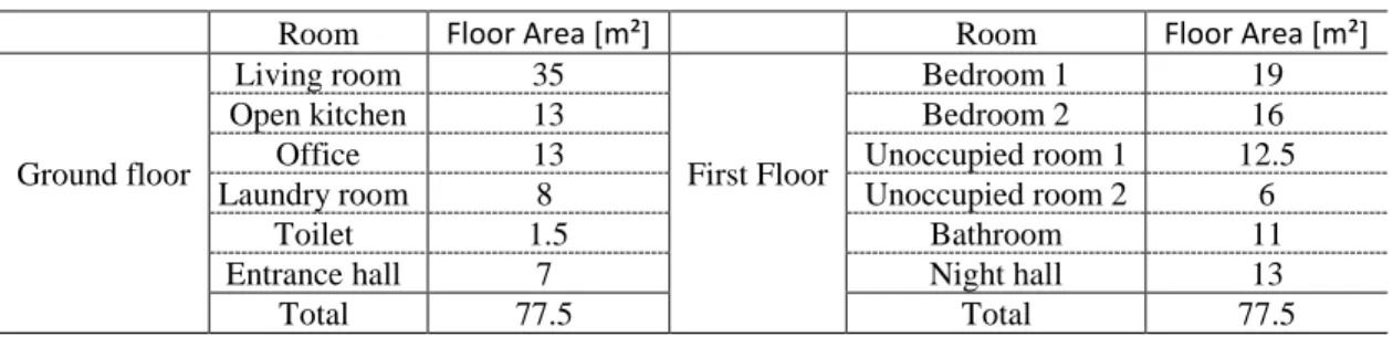
50 value is estimated to be 0.6 vol/h. Table 1 shows the floor areas for the different rooms of the building.Table 1: Floor area for the different rooms
Room Floor Area [m²] Room Floor Area [m²]
Ground floor
Living room 35
First Floor
Bedroom 1 19
Open kitchen 13 Bedroom 2 16
Office 13 Unoccupied room 1 12.5
Laundry room 8 Unoccupied room 2 6
Toilet 1.5 Bathroom 11
Entrance hall 7 Night hall 13
Total 77.5 Total 77.5
Building envelope. The building envelope is light and respects the most recent standards in terms of thermal insulation.
Indeed, it is a wooden structure insulated with 40 cm of sprayed cellulose for the roof and the outer walls. Furthermore, the concrete slab floor is insulated with 65 cm of cellular glass. Finally, the windows consist of triple-glazed windows with aluminum frames with thermal breaks. The global heat transfer coefficient of the building is equal to 0.2 W/m²-K and the K-level (as defined in the Belgian Energy Performance of Buildings Directive (Moniteur belge, 2017)) is equal to 17. Table 2 summarizes the U-values for the different types of walls. The building is consequently efficient from the energetic point of view.
Table 2: U-values for the different types of walls
Wall type Composition Area [m²] U-value [W/m²-K]
Outer wall Wood structure + 40 cm cellulose 158 0.11
Roof Wood structure + 40 cm cellulose 127 0.15
Floor Concrete slab floor + 65 cm cellular glass 82.7 0.1
Window Triple-glazed + aluminum frame 21 0.86
2.2 Description of heating, ventilation and air-conditioning systems
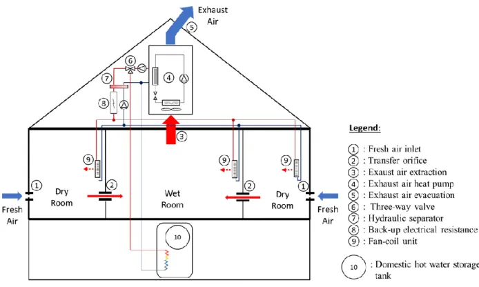
This section describes the heating, ventilation and air-conditioning systems installed in the building. Figure 1 shows a simplified representation of the HVAC systems.
The system consists of a simple exhaust ventilation system combined with a mini exhaust air heat pump used to heat the building and to produce the domestic hot water (4).
The mini exhaust air heat pump (4) is an air-to-water heat pump characterized by an ultra-low heating capacity. Indeed, in order to avoid the frost formation on the evaporator with a volume air flow rate of 200 m³/h, the heating capacity is limited to 1500 W in nominal conditions (A20W35). The refrigerant thermodynamic cycle includes a condenser, an evaporator, a rolling piston compressor and a thermostatic expansion valve. The condenser is a brazed plate heat exchanger and the evaporator is a finned-tube heat exchanger.
3621 Page 3
The heat pump produces hot water that can be either used for the domestic hot water production or for the space heating. The hydraulic circuit connected to the heat pump consists of a three-way valve (6), a domestic hot water storage tank (10), a hydraulic separator (7), a backup electrical resistance (8) and fan-coil units (9) used to heat the building.2.3 Design of the system
The design of the system is a three-step process. Firstly, the aeraulic circuit is designed based on the nominal ventilation airflows. These ventilation airflows are established by the Belgian “Energetic Performance of Buildings” standard. For the presented building case study, the extracted airflows in the bathroom, the toilets, the kitchen and the laundry room are equals to 50, 25, 75 and 50 m³/h, respectively. The total extracted airflow is consequently equals to 200 m³/h. The total supply air is distributed as follows: 42 % in the living, 16 % in the office, 22 % in the bedroom n°1 and 20 % in the bedroom n°2.
In the second step of the design process, the heating capacity of the heat pump is chosen. This one depends on the total ventilation airflow. Three different heat pump sizes are proposed by the manufacturer: 1250 W heating capacity with a ventilation airflow of 150 m³/h, 1500 W heating capacity with a ventilation airflow of 200 m³/h and 1900 W heating capacity with a ventilation airflow of 300 m³/h. In the presented case study, the heat pump with the 1500 W heating capacity is chosen.
In last step of the design process, the electrical power of the backup resistance is chosen. The design is based on the theoretical heating demand of the building with an outside temperature of -10°C and an indoor temperature of 20°C. For the actual case study, the maximum theoretical heating demand is equal to 4100 W. Consequently, a 3000 W backup resistance is chosen.
2.4 Description of HVAC control system
This section describes the control strategies for controlling the ventilation and the heating systems. A good understanding of these control strategies is necessary to analyze correctly the results presented in the next section.
3621 Page 4
A rule-based control is implemented for the ventilation and heat pump strategy. The fan operates continuously, regardless of the building occupancy. Thus, the ventilation air flow rate and the fan electrical consumption are constant and respectively equals 200 m³/h and 55 W.The heat pump can operate in two different modes: the space heating mode and the domestic hot water production mode. The three-way valve controls the heat pump operating mode.
In the “domestic hot water production mode”, the water temperature at the exhaust of the machine varies typically from 35°C (at the beginning of the domestic hot water production process) to 55°C (at the end of the domestic hot water production process). The thermal energy provided by the heat pump is stored in a 200-liter water storage tank situated in the garage. The domestic hot water set-point temperature is 50°C. In the actual control strategy, the domestic hot water production process starts at 11 pm and stops typically at 3 am when the set-point temperature is achieved. The domestic hot water production mode is never activated during the day. It does not create significant comfort issues because the storage tank is oversized compared to the occupant hot water needs.
In “space heating mode”, the water temperature at the exhaust of the machine is almost constant and varies from 40 to 45°C. The heat pump follows a simple ON OFF logic. The control strategy of the heating system is the following. Firstly, the temperature of the living room is measured by a central thermostat. The set-point temperature is fixed at 20°C. When the indoor temperature falls below the set-point, the circulating pump in the hydraulic network is switched on. Secondly, another sensor measures the water temperature at the supply of the heat pump. If the temperature falls below the set-point fixed at 50°C, the machine is switched on. As well, the machine is switched off if the set-point temperature is reached.
Lastly, a 3000 W backup electrical resistance in series with the machine can be switched on if the building heating demand is higher than the heat pump heating capacity. Similarly, the resistance follows a simple ON OFF logic. If the water temperature at the supply of the heat pump decreases over the previous 5 min period, the resistance is activated. The resistance is then switched off if the temperature set-point (fixed at 50°C) at the exhaust of the resistance is reached. Finally, the fan-coil units have their own control logic to adapt the heat emission to reach the room set-point temperature, fixed at 20°C.
3. DESCRIPTION OF THE SYSTEM INSTRUMENTATION
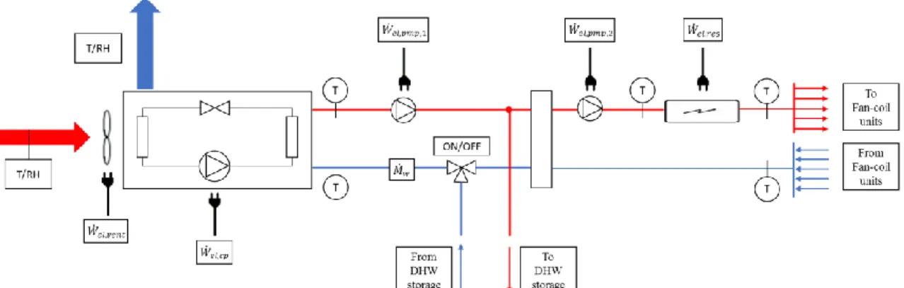
This section describes the different sensors placed in the building to measure the on-site performance of the heat pump. Figure 2 shows the position of the different sensors associated with the heat pump.
In order to measure the performance of the machine and the total electrical consumption of HVAC systems, the following sensors were installed in January 2017:
• Two temperature sensors at the supply and the exhaust of the heat pump, on the water side, • Two temperature sensors at the supply and the exhaust of the back-up electrical resistance, • One temperature sensor to measure the return temperature of the heating system,
• One water flow meter to measure the water volume flow rate at the supply of the machine,
• Three electric meters to measure the compressor consumption, the resistance consumption and the whole system consumption (compressor, resistance and auxiliaries), respectively.
• The weather conditions (temperature, humidity, wind and solar radiation) are retrieved by a weather station connected to the website WeatherUnderground. Its location is close to the house studied (less than 8 km). Moreover, a sensor able to measure the mode (“DHW production mode” or “space heating mode”) of the three-way valve was installed in April 2017. Finally, other sensors, such as temperature and humidity sensors and room temperature sensors were installed in September 2017.
3621 Page 5
Figure 2: Position of the different sensors used to measure the on-site performance of the heat pump
The electrical power consumptions (resistance, compressor and the whole system) are measured by electronic devices (DRS155-D) with a resolution of 1 Wh. The air relative humidities and the air temperatures at the supply and at the exhaust of the heat pump are measured by digital sensors Telaire T9602. The other temperature sensors are digital temperature sensors DS18B20. They are directly put on the wall of the different parts of the heat pump with thermal pad and insulated, except one sensor that is let free in the ambient. Finally, a mechanical volume flow meter with Reed relay output is used to measure the water flow at the supply of the heat pump. It has a resolution of 0.25 liter per pulse. The accuracies of the different devices are listed in Table 3. The data acquisition system is built from a Raspberry Pi that is connected to all these sensors through python software. All the measurements are performed each minute.
Table 3: accuracies of the sensors placed in the building
Measurement Accuracy
Air humidity ±2 %
Air temperature (RH/T sensor) ±0.3 K
Other temperature ±1 K
Temperature difference ±0.2K
Water flow meter ±2 %
Power consumption meter < 1 % (class 1)
4. ANALYSIS OF THE ON-SITE PERFORMANCE
This section presents and analyses the on-site performance of the machine. The results are presented from the 8th of January 2017 until the 2nd of July 2017, i.e from week 2 to week 26. Within this period, the average temperature was near the seasonal normal during winter, from January to February. However, during the springtime (from March to June), the average temperature was much higher than the seasonal normal. The indoor temperature was not measured, but the occupants did not complain about thermal comfort problems. Moreover, due to problems of communication with the unit, the performance for the weeks 3, 7, 8 and 13 are not available. For better readability, the results are presented on a weekly basis.
4.1 Performance in “Domestic hot water production mode”
This section describes the performance of the heat pump in the domestic hot water production mode. Two performance criteria must be analyzed: the thermal energy production of the heat pump and the COP of the machine.
The analysis of the measurements shows that the thermal energy output in DHW production mode varies from 44 to 25 kWh per week during the weeks 14 to 26. Different factors can explain this important variation:
• The outside temperature can influence the energy consumption related to the domestic hot water. Indeed, the domestic hot water storage tank is situated in the garage, out of the building insulated shell. As a result, the storage efficiency decreases when the outside temperature decreases.
• The occupant behavior can have a large impact on the energy consumption related to the domestic hot water. Unfortunately, the sanitary hot water consumption, as well as the water temperature at the supply and at the exhaust of the storage tank were not monitored during this period. Consequently, currently, it is not possible to draw more detailed conclusions about domestic hot water consumption.
3621 Page 6
Contrary to the thermal energy output, the COP of the machine is relatively constant over the weeks. Indeed, the COP varies from 3.36 to 3.59, with an average value of 3.44 (5 % of variation maximum). Indeed, the air flow rate, the supply air temperature and the water mass flow rate are almost constant over time. Consequently, the performance of the machine is constant.
4.2 Consumption of the electrical resistance
This section presents the consumption of the backup electrical resistance. The efficiency of the whole system, which includes the heat pump and the backup resistance, is strongly influenced by the consumption of the resistance. This section presents also the total amount of energy provided by the heat pump and the resistance to the building.
(a) Electrical energy consumption of the backup electrical resistance and thermal energy production of the heat pump in heating mode for weeks 2 to 26
(b) Electrical energy consumption of the resistance and total energy production of the system as a function of the weekly average outside temperature
Figure 3: Energy consumption of the backup electrical resistance on a weekly basis
Figure 3 shows the energy consumption of the backup electrical resistance and the total amount of energy provided by the whole system to the building. The left part of the figure (part (a)) represents the electrical energy consumption of the backup resistance and the thermal energy production of the heat pump in heating mode on a weekly basis. The right part of the figure (part (b)) represents the energy consumption of the backup resistance in kWh on a weekly basis as a function of the weekly average outside temperature. The total amount of energy provided by the whole system (resistance + heat pump) to the building is also represented in Figure 3, part (b). Lastly, the theoretical building energy demand in represented in green in Figure 3, part (b). This theoretical energy demand is calculated considering an overall heat transfer coefficient of 138 W/K, with 70 W/K related to the ventilation, 14 W/K related to the infiltration and 54 W/K related to the transmission losses. These values are based on the building characteristics (the surface areas and the U-values given in Table 4), with a ventilation airflow rate of 210 m³/h and an estimated n50 value of 0.6 vol/h. The energy consumption of the backup electrical resistance varies from 240 to 0 kWh per week during weeks 2 to 26 (see part (a) in Figure 3). From week 2 to week 6, the consumption of the backup resistance is quite high, because the outside temperature is very low at that time of the year. From week 9 to week 19, the consumption of the resistance is lower because the outside temperature is higher at that time of the year. Finally, from week 20 to week 26, the electrical consumption drops to zero.
Contrary to the consumption of the resistance, the thermal energy production of the heat pump in space heating mode is almost constant and is equal to 200 kWh per week (see part (a) in Figure 3).
As shown in Figure 3 (part (b)), the energy consumption of the backup electrical resistance strongly depends on the outside temperature. When the weekly average outside temperature drops below 10°C, the energy consumption of the backup resistance increases linearly when the outside temperature decreases. The slope of the linear regression line (red line in Figure 3, part (b)) is equal to 23.54 kWh/K, corresponding to a heat transfer coefficient of 140 W/K, which is close to the theoretical overall heat transfer coefficient of 138 W/K.
4.3 Consumption of the whole system
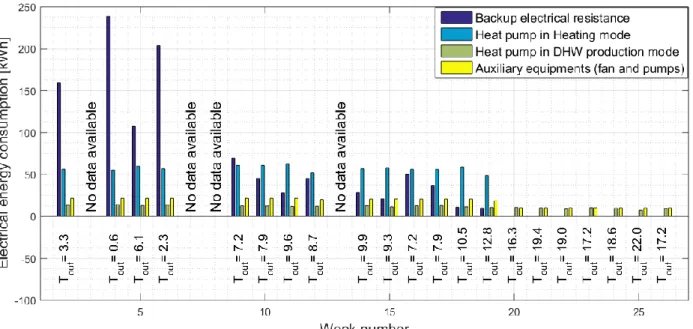
Figure 4 represents the electrical energy consumption in kWh of the backup electrical resistance, the heat pump in heating mode, the heat pump in DHW production mode and the auxiliary equipment on a weekly basis.
3621 Page 7
Figure 4: Electrical energy consumption of the backup electrical resistance, the heat pump in heating mode, the heat
pump in DHW production mode and the auxiliary equipment on a weekly basis
In winter, when the weekly average outside temperature is lower than 7°C, the energy consumption of the resistance is higher than the energy consumption of the heat pump in heating mode. However, in mid-season, when the outside average temperature is comprised between 7°C and 14°C, the opposite phenomenon is observed.
As explained previously, the energy consumption of the heat pump in DHW production mode is a little bit more important in winter than in summer. Moreover, in summer, the energy consumption related to the auxiliary equipment is of the same order of magnitude than the energy consumption of the heat pump in DHW production mode. Indeed, in the actual control strategy, the ventilation operates continuously, leading to a significant fan consumption. The energy consumption of the auxiliary equipment is twice as high in winter than in summer. Indeed, in winter, the heat pump is activated continually for space heating purposes, leading to a high energy consumption of the pumps in the hydraulic network.
4.4 Coverage rate
An important factor that must be determined is the coverage rate of the heat pump. This factor is defined as the thermal energy provided by the heat pump to the building divided by the total thermal energy demand of the building, as given by Eq. 3:
𝜏 = 𝑄𝐻𝑃,𝐷𝐻𝑊,𝑤𝑒𝑒𝑘+ 𝑄𝐻𝑃,𝐻𝑒𝑎𝑡𝑖𝑛𝑔,𝑤𝑒𝑒𝑘 𝑄𝐻𝑃,𝐷𝐻𝑊,𝑤𝑒𝑒𝑘+ 𝑄𝐻𝑃,𝐻𝑒𝑎𝑡𝑖𝑛𝑔,𝑤𝑒𝑒𝑘+ 𝑊𝑟𝑒𝑠,𝑤𝑒𝑒𝑘
(3)
where 𝜏 is the coverage factor on a weekly basis, 𝑄𝐻𝑃,𝐷𝐻𝑊,𝑤𝑒𝑒𝑘 and 𝑄𝐻𝑃,𝐻𝑒𝑎𝑡𝑖𝑛𝑔,𝑤𝑒𝑒𝑘 are respectively the thermal energy output of the heat pump in DHW production mode and in space heating mode in kWh on a weekly basis and 𝑊𝑟𝑒𝑠,𝑤𝑒𝑒𝑘 is the energy consumption of the backup resistance in kWh on a weekly basis.
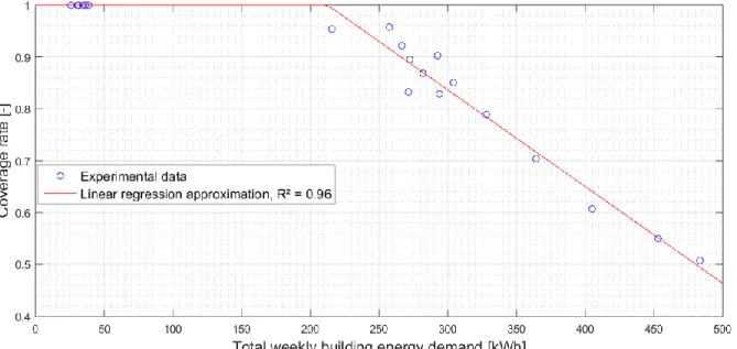
As shown in Figure 5, the coverage factor depends on the total weekly building energy demand. Two different trends can be identified:
•
If the total weekly building energy demand is lower than 210 kWh, the coverage factor is equal to 1. Indeed, in that case, the heating capacity of the heat pump is sufficient, and the machine provides the whole building energy demand.• If the total weekly building energy demand is higher than 210 kWh, the coverage factor decreases linearly when the building energy demand increases. A linear regression approximation (R²=0.96) of the coverage factor as a function of the total weekly building energy demand is given by Eq. 4:
3621 Page 8
𝜏 = 1.3954 − 0.0019 . 𝑄𝐵𝑢𝑖𝑙𝑑𝑖𝑛𝑔,𝑡𝑜𝑡𝑎𝑙,𝑤𝑒𝑒𝑘 (4)
where 𝜏 is the coverage factor on a weekly basis and 𝑄𝐵𝑢𝑖𝑙𝑑𝑖𝑛𝑔,𝑡𝑜𝑡𝑎𝑙,𝑤𝑒𝑒𝑘 is the total weekly building energy demand in kWh. In that case, the coverage factor is lower than 1 because the heating capacity of the heat pump is not sufficient, compared to the total building energy demand. Consequently, the backup electrical resistance is switched on.
Figure 5: Coverage factor of the heat pump as a function of the total weekly building energy demand
5. EXTRAPOLATION OF THE RESULTS FOR STANDARD WEATHER CONDITIONS
The results presented in the previous sections are available from the 8th of January 2017 until the 2nd of July 2017. Within this period, the average temperature was near the seasonal normal during winter, from January to February. However, during the springtime (from March to June), the average temperature was much higher than the seasonal normal. In order to compare the performance of the system with other similar HVAC systems, it has been judged interesting to extrapolate the performance of the system for a typical meteorological year.This section presents the estimation of the performance of the system for a typical meteorological year. The estimation of the heating demand of the building is based on the EPB certificate. This certificate gives the energy consumption and the CO2 emissions of the building for standardized occupancy, indoor climate and weather conditions. The methodology is simple, established on a monthly basis and is based on the energy balanced performed on the whole building. The estimation of the monthly electrical energy consumption of the heat pump and the backup resistance is based on empirical relationships determined in the previous sections. Table 5 summarizes the extrapolation of the results for a typical meteorological year.
The estimation involves the following steps:
• The monthly average outside temperature, the monthly building heating demand and the monthly thermal energy consumption related to the domestic hot water consumption are given by the EPB certificate (column 1, column 2 and column 3 in Table 5).
• The coverage rate of the heat pump, depending on the total monthly building energy demand, is calculated using Equation 4 (column 4 in Table 5). The monthly total amount of thermal energy provided by the heat pump to the building (column 5 in Table 5) is calculated using the coverage rate of the heat pump and the total monthly building energy demand.
• In order to calculate the monthly electrical energy consumption of the heat pump in heating mode (column 9 in Table 5) and in domestic hot water production mode (column 10 in Table 5), a monthly average COP of 3.55 is
3621 Page 9
considered in heating mode and 3.44 in domestic hot water production mode. These values are based on the measured on-site performance.• It is supposed that the monthly thermal energy demand of the building that is not covered by the heat pump is covered by the electrical resistance.
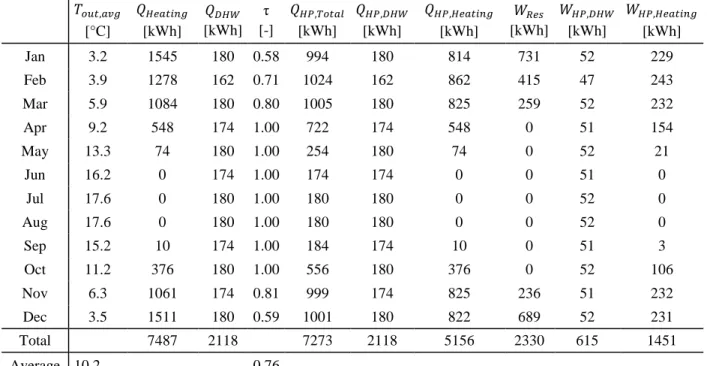
As shown in Table 5, the total energy demand of the building is equal to 9605 kWh per year, with a demand of 7487 kWh in space heating mode and 2118 kWh in domestic hot water production mode. The heat pump provides 76 % of this energy consumption to the building (i.e. 7273 kWh per year) and the other part (i.e. 2330 kWh per week) is covered by the resistance.
Based on this estimation, the seasonal COP of the machine for a typical meteorological year is equal to 2.18. Moreover, by considering a primary energy factor of 2.4, the primary energy efficiency of the whole system is equal to 91 %.
Table 5: Estimation of the monthly building energy demand, the monthly heat pump thermal energy production and
the monthly electrical energy consumption of the heat pump and the backup resistance 𝑇𝑜𝑢𝑡,𝑎𝑣𝑔 [°C] 𝑄𝐻𝑒𝑎𝑡𝑖𝑛𝑔 [kWh] 𝑄𝐷𝐻𝑊 [kWh] τ [-] 𝑄𝐻𝑃,𝑇𝑜𝑡𝑎𝑙 [kWh] 𝑄𝐻𝑃,𝐷𝐻𝑊 [kWh] 𝑄𝐻𝑃,𝐻𝑒𝑎𝑡𝑖𝑛𝑔 [kWh] 𝑊𝑅𝑒𝑠 [kWh] 𝑊𝐻𝑃,𝐷𝐻𝑊 [kWh] 𝑊𝐻𝑃,𝐻𝑒𝑎𝑡𝑖𝑛𝑔 [kWh] Jan 3.2 1545 180 0.58 994 180 814 731 52 229 Feb 3.9 1278 162 0.71 1024 162 862 415 47 243 Mar 5.9 1084 180 0.80 1005 180 825 259 52 232 Apr 9.2 548 174 1.00 722 174 548 0 51 154 May 13.3 74 180 1.00 254 180 74 0 52 21 Jun 16.2 0 174 1.00 174 174 0 0 51 0 Jul 17.6 0 180 1.00 180 180 0 0 52 0 Aug 17.6 0 180 1.00 180 180 0 0 52 0 Sep 15.2 10 174 1.00 184 174 10 0 51 3 Oct 11.2 376 180 1.00 556 180 376 0 52 106 Nov 6.3 1061 174 0.81 999 174 825 236 51 232 Dec 3.5 1511 180 0.59 1001 180 822 689 52 231 Total 7487 2118 7273 2118 5156 2330 615 1451 Average 10.2 0.76
6. CONCLUSIONS
The on-site performance of a mini-exhaust air heat pump integrated into a low energy detached house situated in Belgium has been presented and analyzed.
The results show good performance of the exhaust air heat pump. Indeed, in space heating mode with an average exhaust water temperature of 45°C, the average COP of the machine is equal to 3.55. In DHW production mode, the average COP is equal to 3.44, with a domestic hot water set-point temperature of 50°C. These good performances can be explained by the constant air supply temperature of 20°C and the absence of losses related to defrost cycles. However, due to the limited heating capacity of 1500 W, the exhaust air heat pump is not able to provide the whole energy demand of the building, particularly in winter. Consequently, the electrical backup resistance is activated and the whole system efficiency decreases. A simple annual extrapolation of the results shows an annual coverage factor of 76 % and a seasonal COP of 2.18.
In a future work, different improvements will be proposed in order to increase the annual coverage factor of the heat pump, while maintaining a high seasonal COP. A numerical model of the building and the machine will be developed
3621 Page 10
and calibrated using the on-site performance of the system. Three propositions will be studied using the numerical model:• Firstly, an increase of the heating capacity of the machine would be a good solution to increase the annual coverage factor and the seasonal performance of the whole system. However, increasing the heating capacity while maintaining a constant airflow would create additional losses due to frost formation on the evaporator. Consequently, it would lead to a lower seasonal COP of the machine. To limit the appearance of frost, a modification of the evaporator of the heat pump will also be proposed.
• Secondly, a better regulation of the ventilation system could reduce the annual consumption of the building. Indeed, in highly insulated buildings, the major part of the energy demand is related to the ventilation. Consequently, a demand-controlled ventilation could reduce the energy demand of the building. However, a lower ventilation airflow would also lead to a reduction of the COP of the machine.
• Thirdly, a better regulation of the heating system could increase the seasonal COP of the heat pump. Indeed, the use of a heating curve based on the outside temperature would decrease the average exhaust water temperature of the heat pump and consequently increase the seasonal COP of the machine.
The performance of the whole system depends also on the building insulation level, on the type of building and on the user behavior. Future simulations will show the impact of these parameters.
NOMENCLATURE
COP coefficient of performance (-)EPB energy performance of
buildings Q thermal energy (kWh) RH relative humidity (-) T temperature (°C) W electrical energy (kWh) 𝑊̇ electrical power (W) Subscript avg average cp compressor
DHW domestic hot water
El electrical
HP heat pump
out outside
pump circulator
τ coverage factor (-) res resistance
vent ventilator
week on a weekly basis
REFERENCES
European Commission. (2010). Directive 2010/31/EU of the European parliament and of the council of 19 May 2010 on the energy performance of buildings (recast), Official Journal of the European Union, L 153/13. Retrieved from http://eur-lex.europa.eu/legal-content/EN/TXT/?uri=celex:32010L0031.
European Commission. (2012). Directive 2012/27/EU of the European parliament and of the council of 25 October 2012 on energy efficiency, amending Directives 2009/125/EC and 2010/30/EU and repealing Directives 2004/8/EC and 2006/32/EC, Official Journal of the European Union, L 315/1. Retrieved from http://eur lex.europa.eu/eli/dir/2012/27/oj.
Fracastoro.V, Serraino.M. (2010). Energy analyses of buildings equipped with exhaust air heat pumps (EAHP).
Energy and Buildings, 42 (8), pp 1283–1289.
Liddament M.W., Orme M. (1998). Energy and ventilation. Applied Thermal Engineering,18, pp 1101-1109. Moniteur belge. (2017). Méthode PER – méthode de détermination du niveau de consommation d’énergie primaire des unités résidentielles. Retrieved from https://energie.wallonie.be/fr/exigences-peb-du-1er-janvier-2018-au-31-decembre-2020.html?IDD=114085&IDC=7224.
UCL energy institute. (2017). Final report on analysis of heat pump data from the renewable heat premium payment (RHPP) scheme. Retrieved from https://www.gov.uk/government/publications.
Orme M. (2001). Estimates of the energy impact of ventilation and associated financial expenditures. Energy and